The Classical Model of Type-Token Systems Compared with Items from the Standardized Project Gutenberg Corpus

Abstract

We compare the “classical” equations of type-token systems, namely Zipf’s laws, Heaps’ law and the relationships between their indices, with data selected from the Standardized Project Gutenberg Corpus (SPGC). Selected items all exceed 100,000 word-tokens and are trimmed to 100,000 word-tokens each. With the most egregious anomalies removed, a dataset of 8432 items is examined in terms of the relationships between the Zipf and Heaps’ indices computed using the Maximum Likelihood algorithm. Zipf’s second (size) law indices suggest that the types vs. frequency distribution is log–log convex, with the high and low frequency indices showing weak but significant negative correlation. Under certain circumstances, the classical equations work tolerably well, though the level of agreement depends heavily on the type of literature and the language (Finnish being notably anomalous). The frequency vs. rank characteristics exhibit log–log linearity in the “middle range” (ranks 100–1000), as characterised by the Kolmogorov–Smirnov significance. For most items, the Heaps’ index correlates strongly with the low frequency Zipf index in a manner consistent with classical theory, while the high frequency indices are largely uncorrelated. This is consistent with a simple simulation.

1. Introduction

Type-token systems consist of “types” of object, whose individual occurrences are referred to as “tokens”. In a biological habitat, types might represent species and tokens individual organisms [1,2]. Type-token models have been applied to galactic superclusters [3], the popularity of musical works [4], the sizes of software components [5] and the statistics of written and spoken texts (including dialogues) [6]. In the latter case, unique lexical units (lemmas, wordforms, bi- or trigrams) form types and their specific instances form tokens. The early works of Zipf [7,8], Mandelbrot [9] and Simon [10] have identified underlying power laws, especially the two laws of Zipf and Heaps’ law, whose exponents are supposedly linked by a series of mathematical relationships. We shall call this the “classical model”.

The goal of this paper is to compare this classical model with data extracted from the Standardized Project Gutenberg Corpus (SPGC) [11], which comprises nearly 60,000 works of literature, mostly English, spanning many genres and historical periods. For the purposes of this work, we define types as complete wordforms, regardless of common stems. It thus extends our two earlier papers [12,13] with a larger and more consistent dataset and demonstrates the ranges of applicability of the classical equations. We find the level of agreement depends on the type of literature and the language. For Zipf’s law, the frequency vs. rank characteristic, though generally log–log convex, exhibits a log–log linearity within a limited middle range (ranks 100–1000). Meanwhile, the Heaps’ index correlates strongly with the low frequency Zipf index in a manner consistent with theory. We show that that agrees qualitatively with a simple simulation.

2. Related Work

2.1. The Classical Model

Although Zipf’s first law (the “types” law) was named after George Kingsley Zipf following his famous treatise of 1948 [8], it was known at least 35 years earlier when it was observed in the distribution of city-sizes [14]. It links the frequency $f$ of a type (the number of instances of that type present in the sample) to its “rank” $r$ ($r=1$ being the most frequent type, $r=2$ the second most frequent, etc.):

$$f\left(r\right)\propto {\displaystyle \frac{1}{r^{\alpha }}}$$

(1)

where $\alpha$ (the “Zipf alpha index”) is typically in the region of 1. Figure 1 shows the log–log frequency vs. rank distributions for two typical English texts, showing that $\alpha$ changes significantly between different ranges of $r$. Nevertheless, both exhibit a “middle range” ($100\lesssim r\lesssim 1000$) over which α is approximately constant. The reduced log–log slope for small $r$ is embraced by the Zipf–Mandelbrot law $f\left(r\right)\propto {\displaystyle \frac{1}{{\left(r+m\right)}^{\alpha }}}$ [9], where $m$ is an additional constant. This is asymptotically equivalent to (1) when $r\gg m$.

If word-type selection were statically independent with a probability $\propto 1/r^{\alpha \left(r\right)}$ and no upper limit on $r$, normalisation (the summing of all probabilities to 1) would require $\alpha \left(r\right)>1$ at the upper extremity of $r$, though $\alpha \le 1$ may exist in other regions. Indeed, from an aggregate frequency/rank plot of over 2606 English books, Montemurro [15] observed $\alpha \approx 2.3$ for $r>\mathrm{10,000}$, an effect also seen in the BNC corpus [16] and the Gutenberg corpus for $r>\mathrm{100,000}$ [17]. The switchover between low and high $\alpha$ domains may correspond to the transition from a common kernel lexicon to vocabularies used for specific communications; the latter limited only by the capacity of the human brain [16]. The graphs of Figure 1 relate to individual 100,000-word texts, where discrete plateaux in their upper tails (representing $f=1,2,3$, … etc. [18]) are difficult to interpret in terms of (1). However, there is a strong suggestion of downward “droop” and hence an increasing $\alpha$ with increasing $r$.

Zipf’s second (or “size”) law relates the token frequency $f$ to the number of types $n\left(f\right)$ exhibiting that frequency (i.e., the widths of the low frequency plateaux in Figure 1):

$$n\left(f\right)\propto {\displaystyle \frac{1}{f^{\beta }}}$$

(2)

where the $\beta$, the “Zipf beta index”, is typically between 1 and 2. Like the first law, it predates Zipf’s work and was noted by Corbet in 1941 in a study of Malayan lepidoptera [19]. Figure 2 shows Corbet’s data, indicating $\beta \approx 0.91$ across $1\le f\le 10$, an abnormally low value compared with that of the more typical distribution of the King James Bible also shown ($\beta \approx 1.36$). Simon [10] noted that for both words and biological genera, ${\displaystyle \frac{n\left(1\right)}{n\left(2\right)}}\approx 3$ (corresponding to $\beta \approx 1.58$) with $n\left(1\right)$ comprising approximately half the token population. We note from Figure 2 that while the log–log slopes are approximately constant at low frequencies, extrapolating the law for $f>10$ mostly overestimates the numbers of types at each frequency, suggesting a general log–log convexity (an increasing $\beta$ with increasing frequency). Many authors identify a “low frequency cut-off” $a$ (estimated as 6, 8 and 51 for three different English novels [20]) such that Zipf’s second law is valid only for $f>a$. If this is true, then (despite the obvious appearance of Figure 2) the discretised high frequency portion of the graph may more genuinely follow a power law than the smooth low frequency section. This proposition is examined in Section 4 of this paper.

The third power relationship is Heaps’ (or Herdan’s) law, which is an observed sublinear increase in the total number of types $v\left(t\right)$ as the total number of tokens t increases [21]:

$$v\left(t\right)\propto t^{\lambda }$$

(3)

where the constant $\lambda$, the “Heaps’ index”, lies between zero and one. Figure 3 shows how this law holds roughly across at least two orders of magnitude for two randomly selected documents (one English, the other Finnish).

Although this unbounded increase (seen both in the numbers of hapaxes—types appearing only once—and total types) suggests an infinite accessible vocabulary, this cannot literally be true: a 20-year-old English speaker knows approximately 42,000 word lemmas [22] while the OED of 2020 has 171,476 [13]. Estimating that English lemmas have around four common variations and allowing for proper names and spelling alternatives, the maximum English vocabulary could contain around a million unique wordforms. However, no English text even approaches this: the entire King James Bible has only 12,143 unique wordforms and the aggregate corpus analysed by Montemurro [15] contains no more than 448,359. The latter comprises 2626 volumes, each with its own unique jargon and terminology; one cannot suppose that this comes close to exhausting all possible wordforms, especially as language constantly evolves with the introduction of new words (neologisms). Despite this, $\mathrm{v}\left(t\right) \mathrm{vs}. t$ saturation is seen in ideogrammic languages like Chinese, where the dictionary of semantic characters does have a finite limit [23].

It is often claimed (e.g., [24]) that (2) and (3) are inevitable consequences of (1) with the two indices inextricably linked by the formula:

$$\beta =1+{\displaystyle \frac{1}{\alpha }}.$$

(4)

Similar relationships are proposed to exist between the Zipf $\alpha$ and Heaps’ indices:

$$\lambda ={\displaystyle \frac{1}{\alpha }}$$

(5)

and the Zipf $\beta$ and Heaps’ indices:

$$\lambda =\beta -1.$$

(6)

Under certain assumptions and approximations, these equations are reasonably self-consistent. Lü et al. [25] (amongst others) take (1) as the most fundamental law, describing the selection probability for different types, each characterised by an underlying “rank” $r$ (not necessarily its rank within any given sample). If the discrete nature of the system is ignored, (1) can be represented by a continuous function.

$$f\left(r\right)={\eta r}^{-\alpha }$$

(7)

where $\eta$ is a constant. The frequency range $\delta f$ associated with a small number $\delta r$ of contiguous ranks may now be approximated

$$\delta f=\eta \left[r^{-\alpha }-{\left(r+\delta r\right)}^{-\alpha }\right]\approx \eta \alpha r^{-\alpha -1}\delta r.$$

(8)

Solving (7) for $r$ and substituting into (8) produces ${\displaystyle \frac{\delta r}{\delta f}}\approx {\displaystyle \frac{1}{\alpha }}{\eta }^{{\displaystyle \frac{1}{\alpha }}}{f}^{-\left(1+{\displaystyle \frac{1}{\alpha }}\right)}$, which gives the number of types (ranks) associated with a single frequency $f$ ($\delta f=1$). We thus obtain expressions (2) and (4). Some works (e.g., [3,26]) have taken the opposite approach, making (2) the fundamental law and inferring (1) and (4), though the analysis is largely equivalent. As for Heaps’ law (3), several quite rigorous proofs exist (e.g., [27,28]) but the following provides a useful intuition [25]: loosely interpreting $v\left(t\right)$ as the rank at which $f=1$, we find that (1) can be rewritten $f\left(r\right)={\displaystyle \frac{v^{\alpha }}{r^{\alpha }}}$. Our continuous approximation requires the token population $t$ to equal the integral of this function across $r=1\dots v$:

$$t={\int }_1^{v}f\left(r\right)dr={\displaystyle \frac{v^{\alpha }-v}{\alpha -1}}.$$

(9)

Although this is not analytically solvable for $v$, if $v^{\alpha }\gg v$ then $v\left(t\right)\approx {\left(\alpha -1\right)}^{{\displaystyle \frac{1}{\alpha }}}{t}^{{\displaystyle \frac{1}{\alpha }}}$ which gives (3) and (5). Finally, (6) is obtained by a simple substitution of (5) into (4).

2.2. Critiques of and Alternatives to the Classical Model

The most glaring assumption so far is that the continuous probability distribution (7) provides an adequate approximation for what is in fact a discrete stochastic process. Discrete analysis based on fixed $\alpha$ and unlimited word types [29] shows that although (3) and (5) are valid, (2) and (4) are asymptotically true only for large $f$ [13,30]. At smaller frequencies, $\beta$ is predicted to increase with decreasing $f$, contradicting a general observation that $\beta$ decreases slightly as $f$ approaches 1 [13] (mirroring the low frequency “droop” observed in Figure 1). This effect can be duplicated in the model by imposing an upper limit on the number of accessible types (a “closed vocabulary”), but this is clearly an artificial “fudge” [13,28]. Furthermore, when this model is optimised to fit a random selection of texts, the resulting low frequency $\beta$ exhibits a greater variability than the corresponding directly measured value [13]. When extended beyond the sample to which it was optimised, the model must inevitably predict a rapid decrease in the numbers of low-ranking types as the supply of potential new word types is exhausted. This clearly contradicts the common observation that the numbers of hapax legomena (types represented by only one token) always increase without saturation, as required by Heaps’ law.

A second assumption is that word selection is an independent random process governed by a statical probability distribution. Common sense tells us this cannot be true, since the sample space for each successive word is generally dictated by its predecessors [31]. There are also empirical reasons to be suspicious: during population growth, observed ranks change much more frequently than the model would predict, and their relative frequencies do not always converge towards stable values [24]. Tria et al. [17] point out that (5) is only true under random word selection when $\alpha >1$, and $\alpha \le 1$ would require $\lambda \approx 1$. Furthermore, a very recent paper by Cugini et al. [32] shows that small subsets of ranked random variables tend to approximate the Zipf–Mandelbrot law, whatever their underlying distribution.

There have been many attempts to develop all three laws from an underlying dynamical framework in which the type-selection probability is not static (e.g., [26,33]). These are mostly variants of the Pólya urn model, in which the probability of a type’s future selection increases in proportion to its past selection; the so-called “rich get richer” principle. As early as 1955, Simon [10] showed that if the selection probability of a word type with frequency $f$ is proportional to $n\left(f\right)$, and the generation probability of new word types is constant, then an approximation to Zipf’s second law emerges. This idea has been developed and expanded over several decades, recently by Tria et al. [17], who suggested that the appearance of a new type triggers expansion into an “adjacent possible”, introducing further types not hitherto accessible.

We note these models for the sake of completeness but do not attempt to expand upon them in this paper. We concentrate instead on the classical equations themselves and their relationship with observation.

3. Materials and Methods

As previously noted, $\alpha$ and $\beta$ are not truly constant but vary between different sections of their respective distributions. To investigate the variation of $\beta$ with frequency, we define the seven frequency ranges shown in Figure 4, overlaid upon a typical size/frequency distribution (the Project Gutenberg item PG10, the King James Bible). While the log–log slope ${\beta }_1$ over range 1 (frequencies 1–10) is clearly perceived, the same cannot be said of range 7 (frequencies 64–640) where the underlying continuous curve is obscured by discretisation and random noise. Nevertheless, the Maximum Likelihood (ML) method [34] gives optimum ${\beta }_1\dots {\beta }_7$ for ranges 1 to 7, respectively. Previous observations (see Section 2) suggest a degree of log–log convexity, meaning that (2) will not be strictly valid even within an individual range; nevertheless, if we assume that it is approximately valid then the optimised ${\beta }_s$ may be considered a representative of range $s$ and compared with the values obtained for other ranges.

The following procedure is used to select a “clean” subset of this SPGC, allowing general statistics to be studied with minimal disturbance from unrepresentative and anomalous items.

• To eliminate document length as an interfering variable, all items with less than 100,000 word tokens are rejected. The remainder are trimmed to exactly 100,000 tokens each.
• The item PG4656 Checkmates for Four Pieces by W.B. Fishburne is removed. (This consists almost entirely of chess notation, which is not amenable to iterative process of optimising Maximum Likelihood).
• While most of the remaining data follow a clear “main sequence” (a term we borrow from star classification [35]), anomalies still exist in the $\beta$ data. To classify these consistently we define $k_{i,j}={\prod }_{s=1}^{R}K\left({\beta }_{s,i},{\beta }_{s,j}\right)$ where $K\left(x,y\right)=e^{-{{\displaystyle \frac{1}{2}}\left({\displaystyle \frac{x-y}{\sigma }}\right)}^2}$ is a Gaussian “support” function with standard deviation $\sigma$ and ${\beta }_{s,i}$ is the Zipf index computed for item $i$ over the frequency range $s=1\dots R$ ($R$ in this case being 7). For item $i$, the average support from the other $n-1$ items $k_i={\displaystyle \frac{1}{n-1}}{\sum }_{j=1}^n{k}_{ij}{1}_{i\ne j}$, where $n$ is the total number of items.
• If $k_i<\epsilon$ (where $\epsilon$ is some arbitrary threshold) then item$i$ is classified as anomalous.

Figure 5 shows the cumulative distribution of $k_i$ for four possible values of $\sigma$. The classification clearly depends on $\sigma$ as well as $\epsilon$, and while the choice is ultimately subjective, we use $\sigma =0.15$ since it creates a clear dichotomy at $\epsilon =0.00001$. (Other choices may of course be equally valid).

Of the 57,713-item SPGC, approximately 16% survive this winnowing process and are included in our main study.

Table 1. The seven lowest scoring items by support (anomalies, shown in red) together with the seven highest scoring items (green). EDNN is “Euclidean distance to the nearest neighbour” in 7-dimensional $\beta$-space. We note that anomalies are mostly dictionaries (with vocabularies uncommonly large relative to their token count) while top scoring items include many theological works.

Code	Title (Abbreviated)	Author	$\mathbf{Support}\mathbf{(}{\mathit{k}}_{\mathit{i}}$)	EDNN
PG51155	Dictionary of Synonyms and Antonyms	Samuel Fallows	2.40 × 10−82	2.837
PG22722	Glossary for Spelling of Dutch Language	Matthais de Vries	1.36 × 10−23	1.400
PG10681	Thesaurus of English Words and Phrases	Peter Mark Roget	3.73 × 1018	1.190
PG19704	A Pocket Dictionary: Welsh-English	William Richards	1.71 × 1011	0.841
PG38390	A Dictionary of English Synonyms	Richard Soule	3.38 × 10−10	0.760
PG20738	English-Spanish-Tagalog Dictionary	Sofronio Calderón	1.18 × 10−9	0.721
PG19072	Selected Pamphlets of the Netherlands	-	1.93 × 10−7	0.594
PG23637	The Bishop of Cottontown	John Moore	0.222025	0.0565
PG36909	Memoirs of General Baron de Marbot (v.1)	Baron de Marbot	0.222453	0.0410
PG42645	Expositor’s Bible: Galatians	George Findlay	0.223936	0.0452
PG8069	Expositions of Scripture: Isaiah & Jeremiah	Alexander Maclaren	0.224487	0.0410
PG3434	Social Work of the Salvation Army	Henry Rider	0.224566	0.0023
PG2800	The Koran (English translation)	-	0.224596	0.0023
PG45143	The Way to the West—3 Early Americans	Emerson Hough	0.224600	0.0312

lists the seven anomalies identified at stage 4, along with the seven highest-scoring items.

Figure 6 shows some example plots of $\beta$ for different frequency ranges. We note that while some anomalies appear close to the non-anomalous data, this is an illusion of perspective in 7-dimensional space; the rightmost column of Table 1 shows the shortest Euclidean distance of any anomaly to its nearest neighbour is 0.594, while for the seven highest scoring items, this is at least an order of magnitude lower.

This procedure only removes anomalies manifested in the $\beta$-data, when the full 100,000 tokens of each item are analysed. Remaining anomalies appearing in the $\alpha$ and $\lambda$ indices are considered as and when they arise.

4. Observations on the Zipf $\mathit{\beta }$ Indices

Figure 7a shows the resulting mean values of ${\beta }_1\dots {\beta }_7$ together with the corresponding upper and lower quartiles. While statistical variation is large, the mean $\beta$ shows a gradually slowing increase with increasing frequency, peaking at a little under 2 before falling very slightly at the highest frequency range 7. This agrees with the long-established log–log convexity of $\mathsf{\beta } \mathrm{vs}. f,$ $\beta$ being smallest for the smallest frequencies (though never becoming negative as a closed vocabulary model would require [13]). Figure 6b shows the corresponding KS-significance [36], a measure of how plausibly the distributions follow the power law (1 being the most plausible and 0 the least). Median values and upper and lower quartiles are also shown. Note that when the frequency is low, the median is at 0.7 with an almost maximal interquartile range. As frequency increases, the median rises to a maximum of about 0.9 while the interquartile range narrows. For higher frequencies still, the median falls very slightly with a steady interquartile range; we may suppose that in this region, most items are above the “low frequency cut-off” [20] mentioned in Section 2.1. For the combined range 1–640 (ranges 1–7 combined) only 10% of items have KS-significance exceeding 0.01, and the interquartile range cannot meaningfully be plotted on this scale. Zipf’s second law is therefore approximately valid across the individual ranges but generally does not apply across the entire range of frequencies.

Table 2. Pearson correlation coefficients computed between $\beta$-values for all non-anomalies for frequency ranges $s=1\dots 7$ (See Figure 4). Generally, the closer two ranges are, the more positive the correlation; widely different ranges have weak (though significantly) negative correlation. (Green and yellow highlights indicate $p<0.01$ for positive and negative correlation, respectively).

$\mathit{s}$	1	2	3	4	5	6	7
1	1.000000	0.877568	0.611796	0.302807	0.086714	−0.007730	−0.030490
2	0.877568	1.000000	0.843515	0.517359	0.164752	−0.004763	−0.070956
3	0.611796	0.843515	1.000000	0.791427	0.376716	0.128384	−0.030850
4	0.302807	0.517359	0.791427	1.000000	0.686617	0.347544	0.017829
5	0.086714	0.164752	0.376716	0.686617	1.000000	0.694031	0.151306
6	−0.007730	−0.004763	0.128384	0.347544	0.694031	1.000000	0.442205
7	−0.030490	−0.070956	−0.030850	0.017829	0.151306	0.442205	1.000000

shows a matrix of the Pearson correlation coefficients between $\beta$-values computed across different frequency ranges: adjacent (overlapping) ranges have a strong positive correlation, while those far apart show a very weak negative correlation. For example, a higher than average ${\beta }_7$ tends to accompany a lower than average ${\beta }_1$, which suggests that beneath the noise, size/frequency distributions differ not so much in their absolute slopes but in their respective log–log convexities.

5. Zipf $\mathit{\alpha }$ Indices in the Middle Range

It has long been recognised that Zipf’s frequency/rank law is most accurate in the “middle range”, with major deviations appearing for high and low ranks [24]. However, it is by no means obvious where the boundaries of this “middle range” lie, nor whether a common definition can be applied to different items. Qualitative examination suggests that many items have an approximately log–log linear range (characterisable by a constant $\alpha$ between ranks 100 and 1000, although exceptions can be found). We therefore apply the Kolmogorov–Smirnov (KS) test [36] to the ML frequency vs. rank best-fits for ranks 100–1000, for all the non-anomalous items identified in Section 2. Figure 8 shows the cumulative distribution of KS-significance, along with highlighted items whose frequency/rank distributions are shown in Figure 9. (

Table 3. Bibliographical details of the items in 9 (and highlighted in Figure 8). We note that the three items deviating most from the power law are botanical and entomological treatises (rich in redundant content) while the top scoring items are a Dutch literature essay, a novel and an English translation of Sanskrit epic poem.

Code	Title (Abbreviated)	Author	Language	KS Significance
PG17077	Over literatuur: Critisch en didactisch	M. H. Van Campen,	Dutch	0.999993
PG47629	Ang “Filibusterismo”	Jose Rizal	Filipino	0.134267
PG15476	The Mahabharata Volume 3 (English translation)	-	English	0.0063
PG31558	A Monograph on the Sub-class Cirripedia Vol. 1	Charles Darwin	English	0.000104
PG41782	Moths of the British Isles, First Series	Richard South	English	1.05738 × 10−6
PG39423	Manual of the Botany of the Northern United States	Asa Gray	English	2.6154 × 10−8

lists the bibliographical details of the selected items.) We see that for KS significances greater than about 0.01, the graph has tolerable log–log linearity, whereas lower KS values are indicative of an increasing log–log convexity. Somewhat arbitrarily (based on a qualitative assessment of “what looks right”), we choose a boundary value of 0.03 to classify items into “low” and “high” KS-significance groups, the former comprising the lowest decile.

6. Alpha vs. Beta

Figure 10 shows the indices ${\beta }_1\dots {\beta }_7$ plotted against the corresponding mid-range $\alpha$ for low and high KS significance items, along with the theoretical curve predicted by (4). The correlation coefficient magnitudes for all seven graphs are also shown. Our initial qualitative observations are as follows:

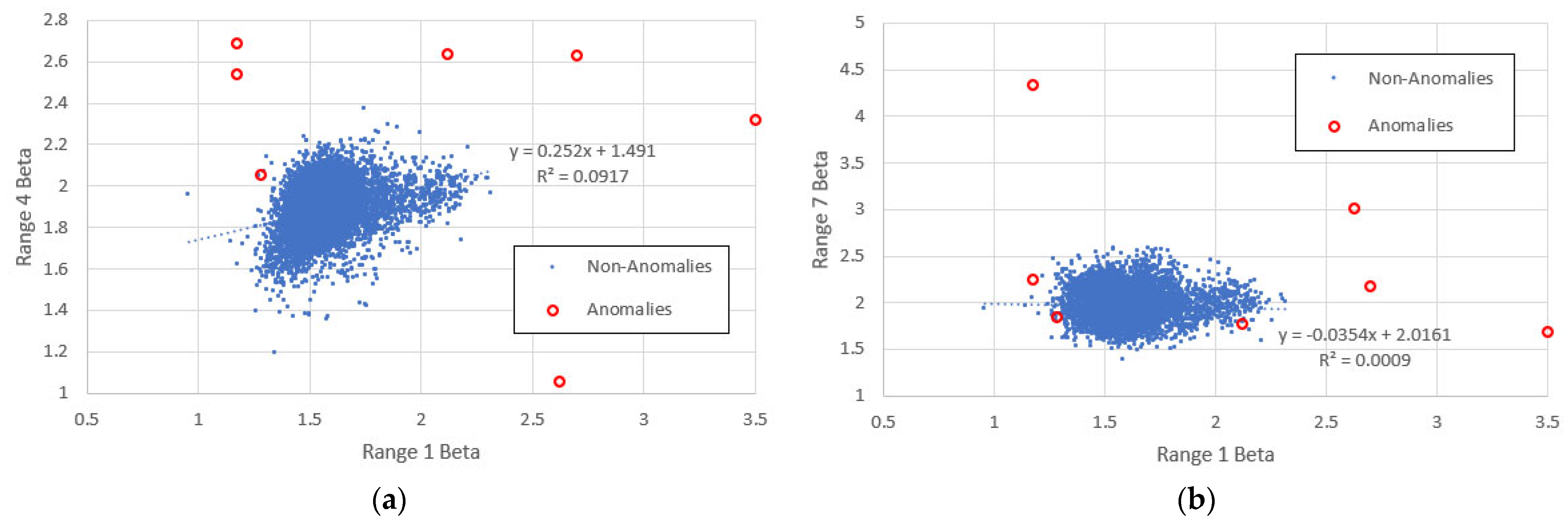
• For the low frequency ranges, the correlation coefficient magnitude is very low. It rises close to unity for range 6, where the frequencies correspond roughly to the middle range ranks across which $\alpha$ was computed. It then falls again in range 7.
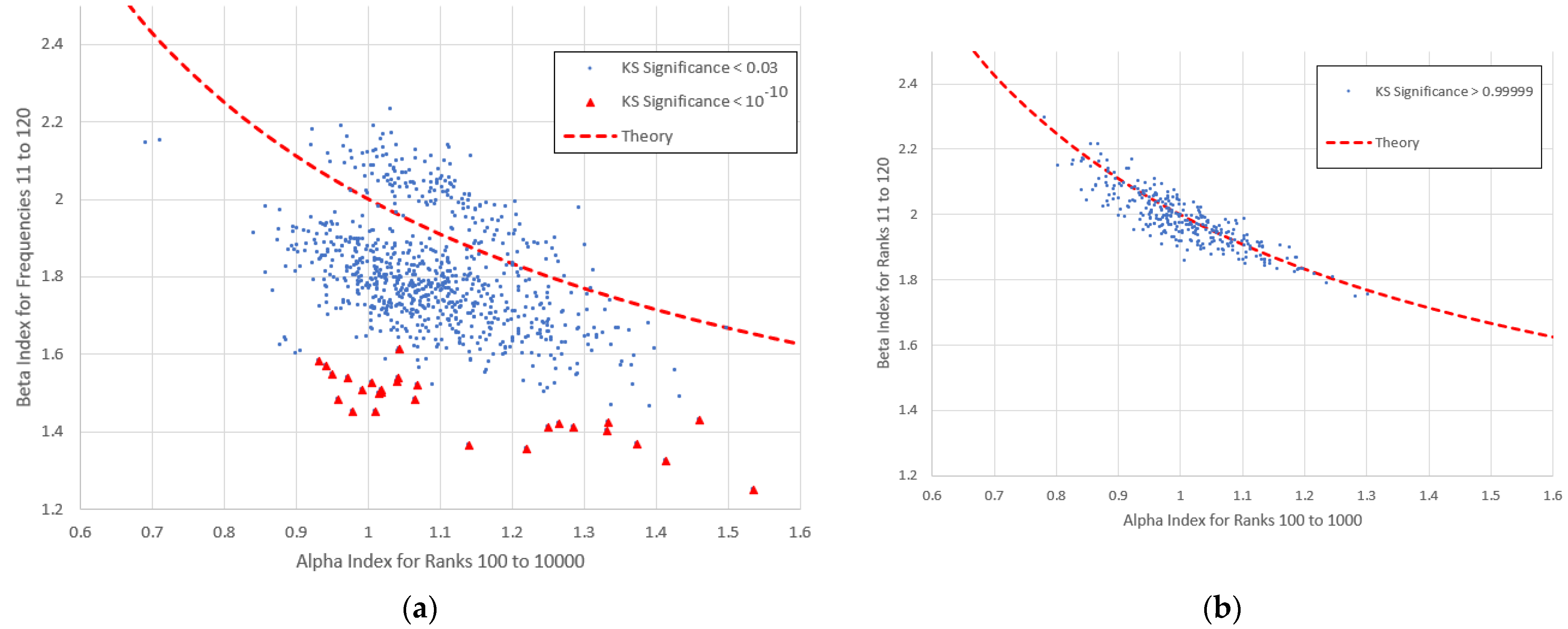
• Agreement with (4) generally improves as the frequencies increase, the best fit being for range 5. Here, items with higher KS-significance are distributed almost symmetrically around the theoretical line, while items with lower KS-significance exist in separate clusters above and below. There is a hint of this behaviour for ranges 4 and 7, though it is curiously absent for range 6.
• For range 1 (and to a lesser extent 2), there is a distinct cluster of high-$\beta$ points, also characterised by a narrower $\alpha$-range than the main population. These points are numerically quite close to the theoretical curve, though they show no obvious indication of following it. Nearly all these items belong to the high KS-significance group and nearly all of them are Finnish (Finnish items appearing almost nowhere else); we therefore refer to this feature as the “Finnish cluster”. The main cluster centred around $\beta =1.6$ is dominated by English items.
• For range 5, there is a distinct “filament” of data points exhibiting low $\beta$, all of which belong to the low KS-significance group. These include many editions of the CIA World Factbook and other works of reference. Since these clearly are not typical linguistic texts, they are of secondary importance to our study.

6.1. The “Finnish Cluster”

For analytical purposes, we define this cluster as containing all items whose indices fall within the rectangle $2<{\beta }_1<2.2$, $0.95<\alpha <1.1$ (shown on Figure 10) and plot the cluster size as a function of a KS-significance limit between 0.01 and 1 (see Figure 11). We find the cluster only exists for KS-significances above 0.048, beyond which its relative size increases approximately linearly with the increasing logarithm of the KS-significance.

Comparison between the Finnish cluster and the main (mostly English) population suggests significant differences between the statistical properties of languages. English is well known for its limited inflexion and agglutination, while Finnish is heavily agglutinated and inflected (more so even than German), giving it a much larger variety of wordforms. Our results also suggest that compared to English, Finnish has a closer adherence to Zipf’s first law (evidenced by the high KS-significance) and a significantly higher $\beta$-index for lower frequencies. We intend to investigate this further, along with the statistical differences between other languages.

6.2. The Middle Range and the “Low Beta Filament”

Frequency range 5 corresponds approximately to the middle range of ranks across which the $\alpha$-indices are measured, as evidenced by the close adherence (at least amongst the high KS-significance data) to the model (4). To obtain a more precise correspondence between the middle range $\alpha$ and $\beta$-index data, we calculate the average upper and lower frequencies corresponding to the rank boundaries $r=100$ and $1000$ across the entire dataset, to obtain a new frequency range $f=11\dots 120$. Figure 12a presents the lower KS-significant data for this new range, showing clear bifircation, with an empty “corridor” through which the theoretical curve runs. The “low beta filament” items clearly have the very lowest KS-significances ($<{10}^{-10}$), supporting our earlier suggestion that they are highly atypical texts. Meanwhile, Figure 12b shows that the highest KS-significant data ($>0.99999$) are those in closest agreement with (4).

7. Vocabulary Growth and Heaps’ Law

So far, we have applied Zipf’s first and second laws to documents with a fixed length of 100,000 word tokens. Meanwhile, Heaps’ law (3) describes the growth of documents and is theoretically linked to Zipf’s laws by (5) and (6). An optimum Heaps’ index was obtained for each item by iteratively adjusting $\lambda$ to minimise the mean square difference between (3) and the measured vocabulary profile across 100 intervals of 1000 tokens each. Figure 13 shows the cumulative frequency distributions for optimised Heaps’ indices obtained for items with high and low KS-significance. Our first observation is that for the low KS-significant items, the average Heaps’ index is significantly lower than for the high KS-significant items, with a larger standard deviation.

Figure 14 shows $\lambda$ plotted against $\beta$ for the seven frequency ranges, compared with the prediction of (6), again separating the high and low KS-significance groups. For range 1, the data in both groups are strongly correlated, with the bulk of points roughly following the theoretical curve. Nevertheless, the items in the “Finnish cluster” (which have a considerably higher than average $\lambda$) lie well above the theoretical prediction. As the frequencies increase, the correlation coefficient gradually falls as correspondence with (6) is lost. This makes sense, since $\lambda$ is associated with the rate at which new types (frequency $f=1$) appear and would be associated with the lowest frequency statistics.

In addition to this, however, vocabulary growth is retarded by the reappearance of existing types, so one would expect some correlation with higher frequency statistics. To investigate this potential effect, we propose a simplified model to represent the frequency-rank distribution and obtain the corresponding profile of vocabulary growth. To represent the imperfect adherence to Zipf’s first law, we propose an $\alpha$-value which changes abruptly at some rank $r=\rho$, from a high frequency value ${\alpha }_{hf}$ to a low frequency value ${\alpha }_{lf}$:

$$f\left(r\right)=\left\{\begin{array}{cc}{\displaystyle \frac{v^{{\alpha }_{lf}}}{{\rho }^{{\alpha }_{lf}-{\alpha }_{hf}}{r}^{{\alpha }_{hf}}}};& r<\rho \\ {\displaystyle \frac{v^{{\alpha }_{lf}}}{r^{{\alpha }_{lf}}}};& r\ge \rho \end{array}\right..$$

(10)

Substituting (10) into (9), we obtain an expression for the token population $t$:

$$t={\displaystyle \frac{v^{{\alpha }_{lf}}}{{\rho }^{{\alpha }_{lf}-{\alpha }_{hf}}}}{\displaystyle \frac{{\rho }^{1-{\alpha }_{hf}}-1}{1-{\alpha }_{hf}}}+v^{{\alpha }_{lf}}{\displaystyle \frac{v^{1-{\alpha }_{lf}}-{\rho }^{1-{\alpha }_{lf}}}{1-{\alpha }_{lf}}}$$

(11)

where following (4), we define high and low frequency $\beta$ indices ${\beta }_{hf}=1+{\displaystyle \frac{1}{{\alpha }_{hf}}}$ and ${\beta }_{lf}=1+{\displaystyle \frac{1}{{\alpha }_{lf}}}$, respectively, which have no strong correlation with each other (Table 2).

The simulation procedure is as follows:

• Generate ${\beta }_{hf}$ and ${\beta }_{lf}$ as independent Gaussian random variables subject to the constraint ${\beta }_{hf}-{\beta }_{lf}<0.15$, thus ensuring a minimum log–log convexity of $n\left(f\right)$ vs. $f$. The chosen mean values are 1.9 and 1.6, respectively (roughly the middle values for ranges 1 and 7, see Figure 10) and both standard deviations are 0.15.
• Compute the corresponding $\alpha$-indices, ${\alpha }_{hf}={\displaystyle \frac{1}{{\beta }_{hf}-1}}$ and ${\alpha }_{lf=}{\displaystyle \frac{1}{{\beta }_{lf}-1}}$.
• Use (11) to compute the profile of $\mathrm{v} \mathrm{vs}. t,$ using 100 steps of 1000 tokens. (The transitional rank $\rho$ is set to 1000, this being the upper limit of the middle range as defined in Section 5).
• Compute the optimal value of $\lambda$ in (3) to fit this profile by minimising the mean square error.
• Repeat these four steps 500 times and plot optimised $\lambda$ vs. ${\beta }_{hf}$ and ${\beta }_{lf}$.

Figure 15 shows the results. While${\beta }_{hf}$ shows weak though nevertheless significant correlation with $\lambda$ (as in the experiment), ${\beta }_{lf}$ strongly correlated and approximately follows (6) (though deviating somewhat for large $\lambda$). In the latter case, statistical scatter is much less than observed in Figure 14, though this is to be expected in a simplified model with fewer extraneous variables than the reality. The parallelism between the bases of the ranges 4–7 clusters in Figure 14 is reproduced in Figure 15, where it is clearly related to log–log convexity (i.e., ${\beta }_{hf}<{\beta }_{lf}$; note that if ${\beta }_{hf}={\beta }_{lf}$, then (11) would become identical to (9) and all points would lie on the theoretical line). While this simulation is by no means precise, it nevertheless provides a qualitative insight into the observed behaviour of the real texts.

8. Discussions and Conclusions

This paper examines the agreement between data taken from the Standardized Project Gutenberg Corpus (SPGC) and the classical type-token equations used by (amongst many others) Kornai [24] and Lü et al. [25]. Items selected for study are all truncated to exactly 100,000 word tokens, and the Zipf $\beta$ indices are computed across seven logarithmically spaced frequency ranges. Outliers are identified in terms of their lack of proximity to other data-points by means of a Gaussian support function and eliminated from the main study. Our findings can be summarised as follows.

• Outlying items identified in the $\beta$-data are nearly all dictionaries, while items with the highest support are dominated by religious works.
• Although wide statistical variations exist, the average $\beta$ index generally increases with increasing frequency, corresponding to a log–log convexity of the types vs. frequency distribution.
• The $\beta$ indices measured for closely overlapping frequency ranges show a strong positive correlation, while those for frequency ranges widely separated show a weak negative correlation. (For example, if $\beta$ is above average in the frequency range 1 to 10, then it is likely to be below average in the range 64–640),
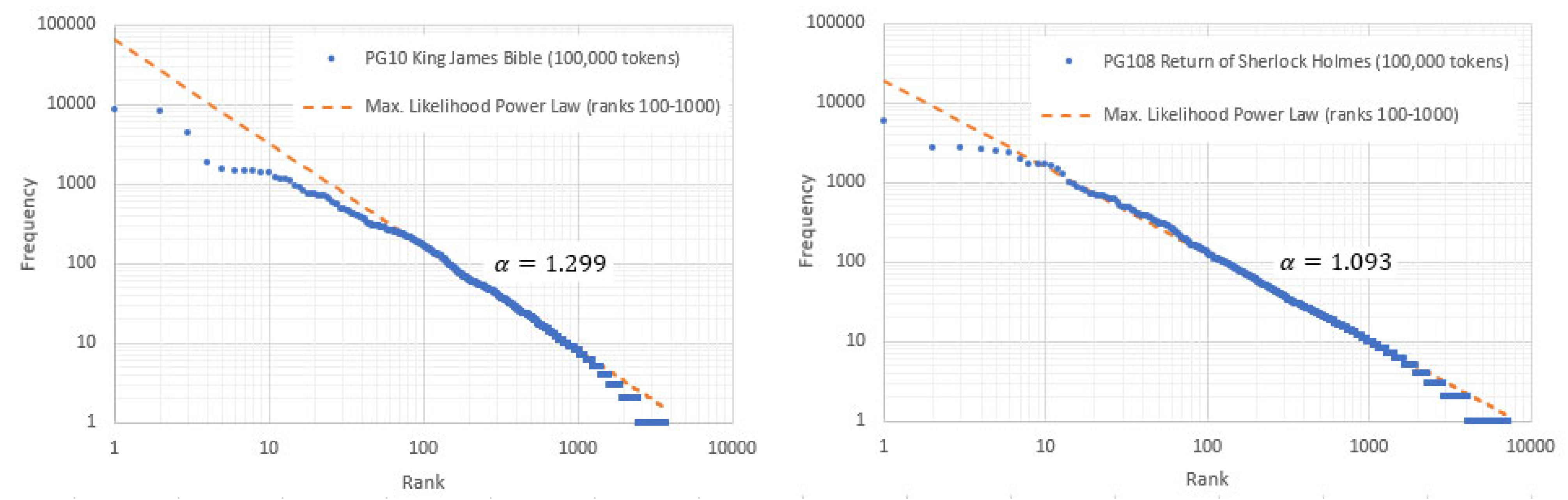
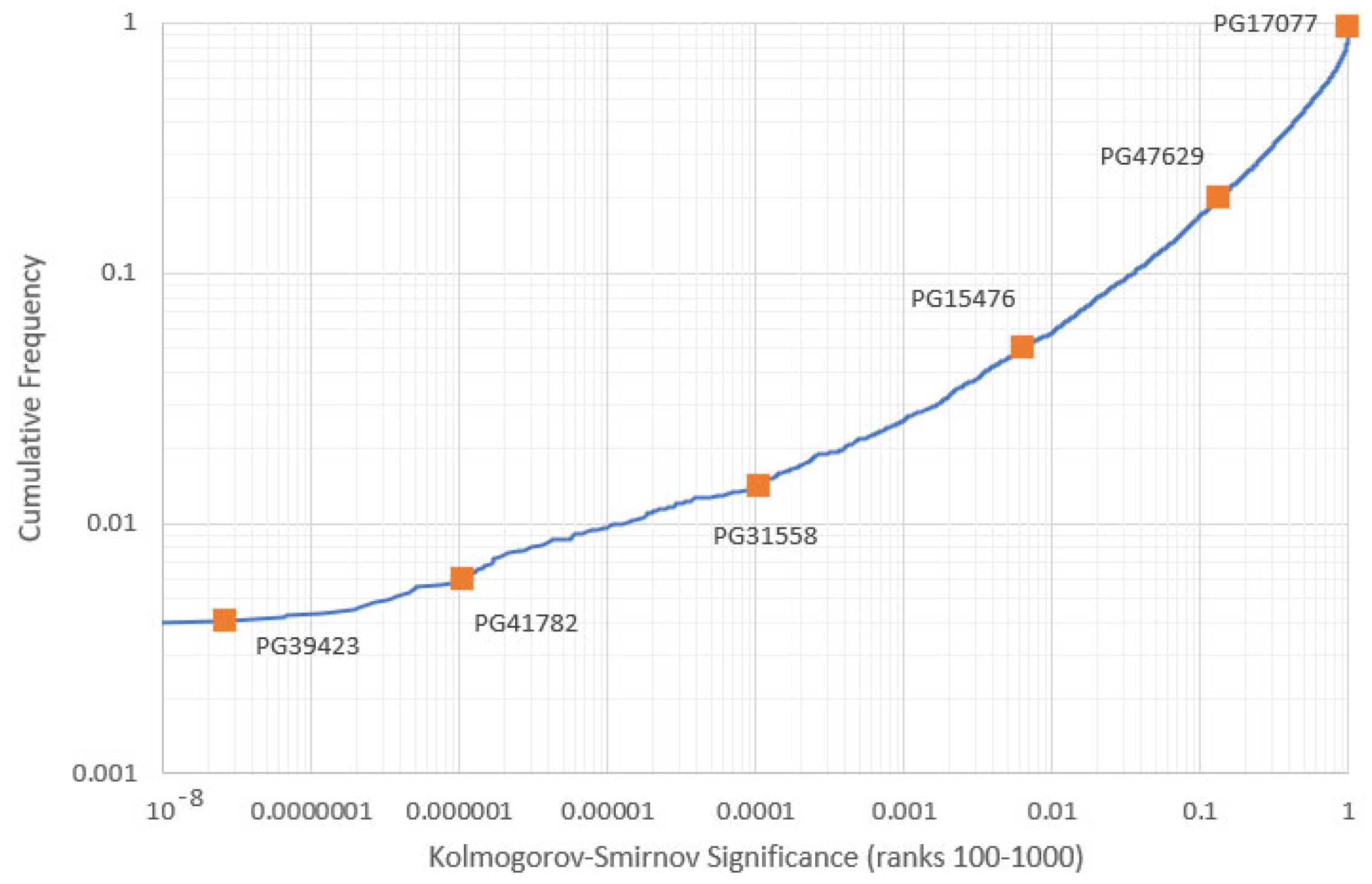
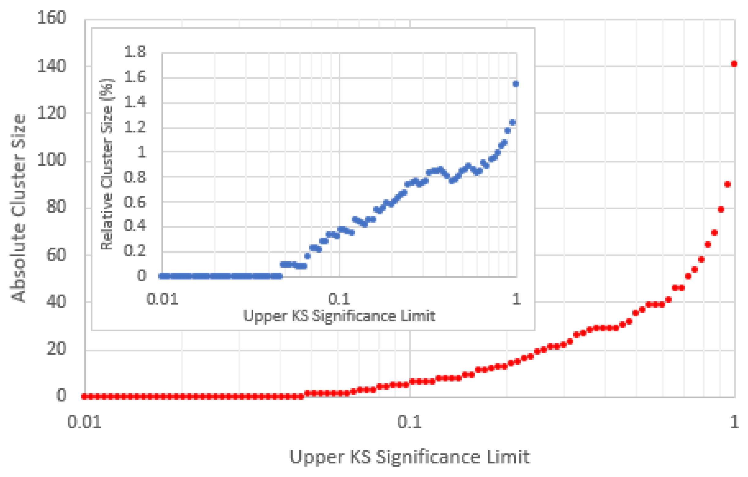
• Adherence to Zipf’s first law across the middle range (defined as the interval between ranks 100 to 1000 inclusive) may be characterised by the Kolmogorov–Smirnov (KS) significance.
• When the frequency range used to compute $\beta$ corresponds roughly to the previously defined middle range, the points roughly follow the classical Equation (4). Of these, items with the highest KS-significance follow the equation most closely (Figure 12).
• Two notably anomalous phenomena appear in the plots of $\mathsf{\beta } \mathrm{vs}. \mathsf{\alpha }.$ Firstly, for range 1 (frequencies 1 to 10), there exists a distinct secondary cluster of points, all with high $\beta$ and all of which have high KS-significance (>0.048). Nearly all of these are Finnish, and Finnish items appear almost nowhere outside this cluster. Secondly, for frequencies corresponding to the middle range, we note a “filament” of low-$\beta$ points, all of which have especially low KS-significance (${<10}^{-10}$). All of the latter are reference books.
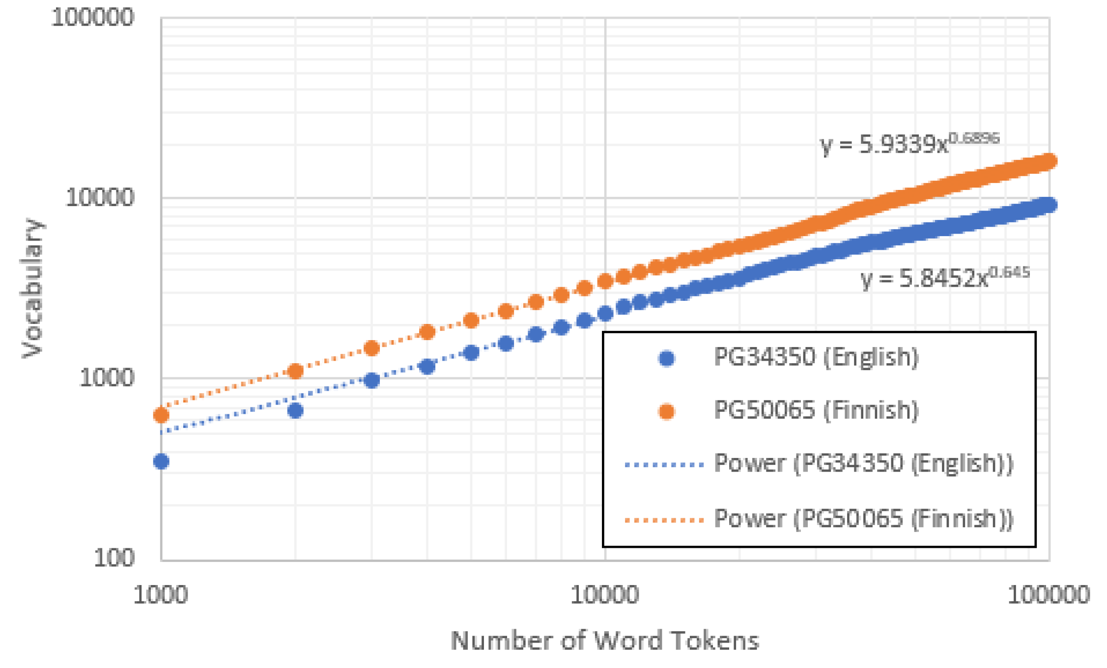
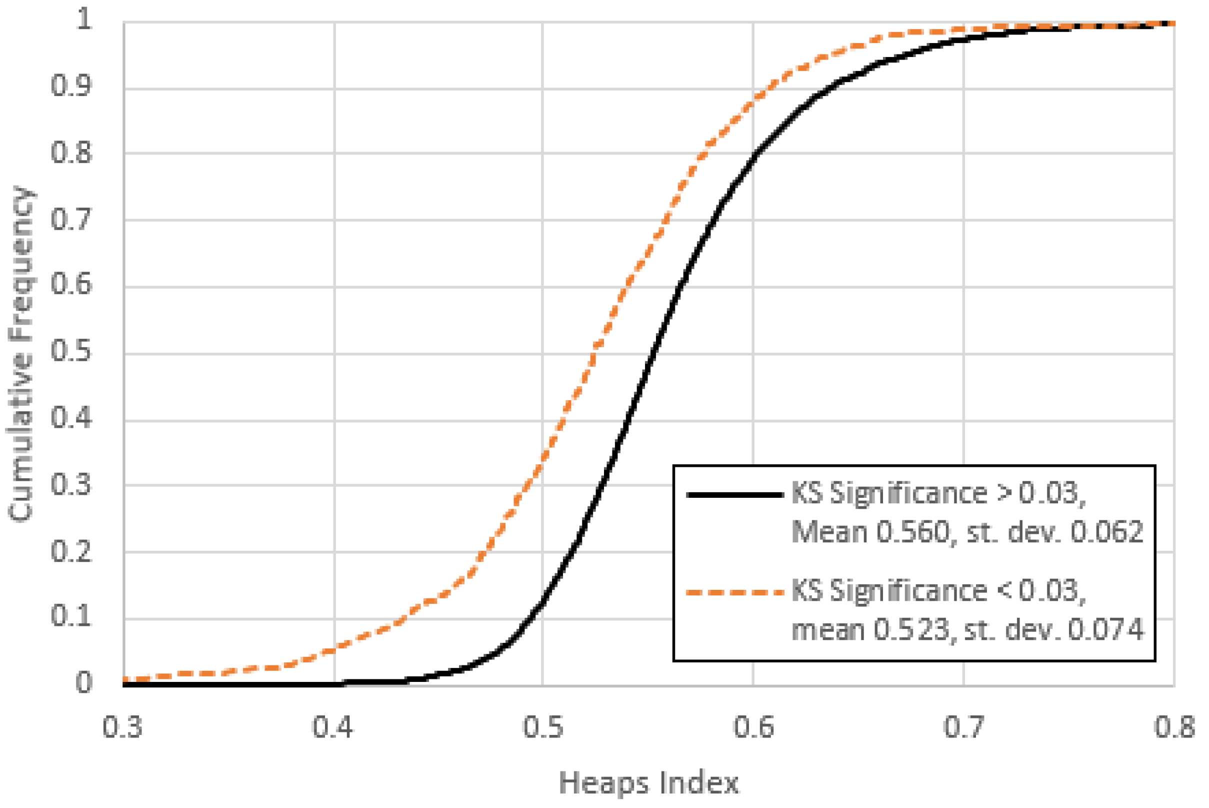
• For the lowest frequency range, the $\beta$ index correlates strongly with the optimised Heaps’ index $\lambda$ in a manner roughly consistent with Equation (6). (The Finnish items noted in point 6 are an exception.) This correlation gradually disappears as the frequencies increase.
• A simplified model based upon an abrupt change in $\alpha$ and $\beta$ between high and low frequencies (to create a convex distribution) reproduces the basic features observed in the data. We note that the Heaps’ index is largely dependent on the statistics of the lowest-frequency types and is affected only weakly by the high frequency indices.

While all these points merit further study, we are particularly fascinated by the dichotomy between the Finnish items and the main body of data (mostly English). We are furthermore interested to discover if other languages have similar peculiarities, such as those documented by Yang and Xiangyi [37], and what mathematical models can be used to describe their behaviour. The SPGC has a paucity of Finnish: our selection (based on document length and $\beta$-statistics alone) contains only 165 Finnish items, compared to 7932 items in English. We therefore intend to compile a much larger corpus of items in Finnish and other languages in order to investigate further.

References

1. Mora, C.; Tittensor, D.P.; Adl, S.; Simpson, A.G.B.; Worm, B. How Many Species are there on Earth and in the Ocean? PLoS Biol. 2011, 9, e1001127. [Google Scholar] [CrossRef] [PubMed]
2. Costello, M.; Wilson, S.; Houlding, B. Predicting Total Global Species Richness using Rates of Species Description and Esitmates of Taxonomic Effort. Syst. Biol. 2012, 61, 871–883. [Google Scholar] [CrossRef] [PubMed]
3. de Marzo, G.; Labini, D.; Pietronero, L. Zipf’s Law for Cosmic Structures: How Large are the Greatest Structures in the Universe? Astron. Astrophys. 2021, 651, A114. [Google Scholar] [CrossRef]
4. Dodd, J.; Letts, P. Types, Tokens, and Talk about Musical Works. J. Aesthet. Art Crit. 2017, 75, 249–1963. [Google Scholar] [CrossRef]
5. Hatton, L. Power-Law Distributions of Component Size in General Software Systems. IEEE Trans. Softw. Eng. 2009, 35, 566–572. [Google Scholar] [CrossRef]
6. Linders, G.; Louwerse, M. Zipf’s Law Revisited: Spoken Dialog, Linguistic Units, Parameters and the Princip. Psychon. Bull. Rev. 2023, 30, 77–101. [Google Scholar] [CrossRef]
7. Zipf, G. The Unity of Nature, Least-Action, and Natural Social Science. Sociometry 1942, 5, 48–62. [Google Scholar] [CrossRef]
8. Zipf, G. Human Behaviour and the Principle of Least Effort; Addison-Wesley: Cambridge, MA, USA, 1949. [Google Scholar]
9. Mandelbrot, B. An informational theory of the statistical structure of language. In Communication Theory; Jackson, W., Ed.; Butterworths Scientific Publications: London, UK, 1953; pp. 486–502. [Google Scholar]
10. Simon, H.A. On a Class of Skew Distribution Functions. Biometrika 1955, 42, 425–440. [Google Scholar] [CrossRef]
11. Gerlach, M.; Fon-Clos, F. A Standardized Project Gutenberg Corpus for Statistical Analysis of Natural Language and Quantitative Linguistics. Entropy 2020, 22, 126. [Google Scholar] [CrossRef]
12. Tunnicliffe, M.; Hunter, G. The Predictive Capabilities of Mathematical Models for Type-Token Relationships in English Language Corpora. Comput. Speech Lang. 2021, 70, 101227. [Google Scholar] [CrossRef]
13. Tunnicliffe, M.; Hunter, G. Random Sampling of the Zipf-Mandelbrot Distribution as a Representation of Vocabulary Growth. Physica A 2022, 608, 128259. [Google Scholar] [CrossRef]
14. Auerbach, F. The Law of Population Concentration. EPB Urban Anal. City Sci. 2023, 50, 290–298. [Google Scholar] [CrossRef]
15. Montemurro, M. Beyond the Zipf-Mandelbrot Law in Quantitative Linguistics. Physica A 2021, 300, 567–578. [Google Scholar] [CrossRef]
16. Ferrer-i-Cancho, R.; Sole, R. Two Regimes in the Frequency of Words and the Origin of Complex Lexicons: Zipf’s Law Revisited. J. Quant. Linguist. 2001, 8, 165–173. [Google Scholar] [CrossRef]
17. Tria, F.; Loreto, V.; Servedio, V. Zipf’s, Heaps’ and Taylor’s Laws are Determined by the Expansion into the Adjacent Possible. Entropy 2018, 20, 752. [Google Scholar] [CrossRef] [PubMed]
18. Bolea, S.; Pirnau, M.; Bejinariu, S.; Apopei, A.; Gifu, D.; Teodorescu, H.-N. Some Properties of Zipf’s Law and Applications. Axioms 2024, 13, 146. [Google Scholar] [CrossRef]
19. Corbet, S.A. The Distribution of Butterflies in the Malay Peninsula (Lepid.). Proc. R. Ent. Soc. Lond. (A) 1941, 16, 101–116. [Google Scholar] [CrossRef]
20. Corral, A.; Bolenda, G.; Ferrer-i-Cancho, R. Zipf’s Law for Word Frequencies: Word Forms versus Lemmas in Long Texts. PLoS ONE 2015, 10, e0129031. [Google Scholar] [CrossRef]
21. Herdan, G. Type-Token Mathematics: A Textbook of Mathematical Linguistics; Mouton: The Hague, The Netherlands, 1960. [Google Scholar]
22. Brysbaert, M.; Stevens, M.; Mandera, P.; Keuleers, E. How Many Words Do We Know? Practical Estimates of Vocabulary Size Dependent on Word Definition, Degree of Language Input and the Participant’s Age. Front. Psychol. 2016, 7, 1116. [Google Scholar] [CrossRef]
23. Dahui, W. True Reason for Zipf’s Law in Language. Physica A 2005, 358, 545–550. [Google Scholar] [CrossRef]
24. Kornai, A. Zipf’s Law Outside the Middle Range. In Proceedings of the 6th Meeting on Mathematics of Language, Orlando, FL, USA, 23–25 July 1999. [Google Scholar]
25. Lü, L.; Zhang, Z.-K.; Zhou, T. Zipf’s Law Leads to Heaps’ Law: Analysing their Relation in Finite-Sized Systems. PLoS ONE 2010, 5, e14139. [Google Scholar] [CrossRef] [PubMed]
26. de Marzo, G.; Gabrielli, A.; Pietronero, L. Dynamical Approach to Zipf’s Law. Phys. Rev. Res. 2021, 3, 013084. [Google Scholar] [CrossRef]
27. van Leijenhorst, D.; van der Weide, T. A Formal Derivation of Heaps’ Law. Inf. Sci. 2005, 170, 263–272. [Google Scholar] [CrossRef]
28. Evert, S. A Simple LNRE Model for Random Character Sequences. Proc. JADT 2004, 2024, 411–422. [Google Scholar]
29. Mandelbrot, B. On the Theory of Word Frequencies and on Related Markovian Models of Discourse. In Structure of Language and its Mathematical Aspects; Jakobson, R., Ed.; American Mathematical Society: Providence, RI, USA, 1961; pp. 190–219. [Google Scholar]
30. Corral, Á.; Serra, I.; Ferrer-i-Cancho, R. Distinct Flavours of Zipf’s Law and its Maximum Likelihood Fitting: Rank-Size and Size-Distribution Representations. Phys. Rev. E 2020, 102, 052113. [Google Scholar] [CrossRef]
31. Thurner, S.; Hanel, R.; Liu, B.; Corominas-Murtra, B. Understanding Zipf’s Law of Word Frequencies through Sample-Space Collapse in Sentence Formation. J. R. Soc. Interface 2015, 12, 20150330. [Google Scholar] [CrossRef]
32. Cugini, D.; Timpanaro, A.; Livan, G.; Guarnieri, G. Universal Emergence of Local Zipf-Mandelbrot Law. 2025. Available online: https://arxiv.org/html/2407.15946v2 (accessed on 12 May 2025).
33. Zanette, D.H.; Montemurro, M.A. Dynamics of Text Generation with Realistic Zipf’s Distribution. J. Quant. Linguist. 2005, 12, 29–40. [Google Scholar] [CrossRef]
34. Bauke, H. Parameter Estimation for Power-Law Distributions by Maximum Likelihood Methods. Eur. Phys. J. B 2007, 58, 167–173. [Google Scholar] [CrossRef]
35. ANTF. The Hertzsprung-Russell Diagram, Commonwealth Scientific and Industrial Research Organization. Available online: https://www.britannica.com/science/Hertzsprung-Russell-diagram (accessed on 15 July 2024).
36. Press, W.H.; Teukolsky, S.A.; Vetterling, W.T.; Flannery, B.P. Numerical Recipes in C: The Art of Scientific Computing, 2nd ed.; Cambridge University Press: Cambridge, UK, 1992. [Google Scholar]
37. Yang, Z.; Xiangyi, Z. The Applicability of Zipf’s Law in Report Text. Lect. Notes Lang. Lit. Clausius Can. 2023, 6, 57–64. [Google Scholar]
Figure 1. Frequency f   vs .   r a n k r for two typical English texts. While the log–log slope α varies between different ranges of r , it remains approximately constant in the “middle range” ( 100 r 1000 ) where it is marginally greater than unity. For ranks above the middle range, each graph discretises into a series of plateaux, each representing a particular value of f . Both graphs suggest the beginnings of a downward “droop” in this region.
Analytics 04 00016 g001
Figure 2. Types vs. frequency plot for Corbet’s butterfly data [19] and the King James Bible (data collected by the authors), both exhibiting the Zipf size law.
Analytics 04 00016 g002
Figure 3. Heaps’ vocabulary plots for typical English and Finnish texts, with best fit power laws overlaid. (In the equation, x represents word tokens and y vocabulary).
Analytics 04 00016 g003
Figure 4. Typical types vs. frequency distribution (PG10: King James Bible, first 100,000 tokens) with frequency ranges overlaid. The Zipf β indices across these ranges were computed using the maximum likelihood estimation (MLE) for all 9312 selected corpus items.
Analytics 04 00016 g004
Figure 5. Cumulative distributions of the neighbour support, for all items, using four different values of σ . The most extreme outliers are trimmed from the left, as (even on a logarithmic scale) their inclusion would have intolerably compressed the right-hand portion of the distribution.
Analytics 04 00016 g005
Figure 6. Example scatter plots of β obtained using different frequency ranges for items classified as anomalies and non-anomalies. The algorithm rejects egregious anomalies while accepting most plausible outliers. (a) Low and medium frequency ranges show a strong positive correlation, while (b) low and high frequency ranges exhibit a weak negative correlation (see also Table 2).
Analytics 04 00016 g006
Figure 7. (a) Median and upper and lower quartile Zipf β indices computed for all seven frequency ranges and for the complete range 1–640. (b) KS significance information for the β values, showing the mean and the upper and lower quartiles. The values for the frequency range 1–640 are too small to be shown meaningfully on the graph and are quoted a text box.
Analytics 04 00016 g007
Figure 8. Part of the cumulative frequency distribution of KS significance values obtained from ML power law fitting to ranks 100–1000, for 100,000 tokens for all PG items previously classified as non-anomalies. KS-significance represents the strength of the null hypothesis that the power law is true. Items whose distributions are shown in Figure 9 are highlighted. (The leftmost portion of the graph is truncated for greater clarity: the lowest KS significance recorded is 2.65 × 10 46 for PG14, The 1990 CIA World Factbook).
Analytics 04 00016 g008
Figure 9. Frequency/rank distributions for six PG items with different KS significances for the ML power law computed across ranks 100–1000 for 100,000 tokens. Smoothed curves were obtained using logarithmic binning. (See also Figure 8).
Analytics 04 00016 g009
Figure 10. Non anomalous β 1 β 7 plotted against mid-range α ( 100 r 1000 ) for log–log linear KS significance below and above 0.03. Lower right graph shows the variation in the Pearson correlation coefficients across the different frequency ranges.
Analytics 04 00016 g010
Figure 11. Number of items in the “Finnish cluster” in range 1 (frequencies 1–10) found amongst items below a variable maximum KS-significance for mid-range α . The cluster disappears amongst items with KS-significance below 0.048, beyond which it increases with the KS-significance until the latter approaches 1. The inset graph shows cluster size relative to the total number of items below the KS-significance limit, the maximum being approximately 1.55%.
Analytics 04 00016 g011
Figure 12. Comparison of mid-range α and β for frequencies 11 to 120 (the average frequency range corresponding to the rank range 100 to 1000 used in the α calculations) with theoretical curve of (4). (a) All items with KS-significance below 0.03 (those below 10 10 highlighted in red) and (b) items with KS-significance exceeding 0.99999.
Analytics 04 00016 g012
Figure 13. Cumulative frequency distributions for optimised Heaps’ indices obtained for items with high and low KS-significance of α in the middle range. We note that for the low KS-significance items, the average Heaps’ index is significantly lower, with a larger standard deviation.
Analytics 04 00016 g013
Figure 14. Non-anomalous Heaps’ index λ plotted against corresponding β for all seven frequency ranges. Items with KS-significance of α in the middle range are differentiated. Lower right graph shows the variation in the Pearson correlation coefficients across the different frequency ranges.
Analytics 04 00016 g014
Figure 15. Scatter plots of (a) low and (b) high frequency β indices vs. the optimised Heaps’ index obtained by simulation using the simplified model of (10) and (11). We note the qualitative agreement between these and the real results of Figure 14. Results are based on 500 independent simulations.
Analytics 04 00016 g015