A Longitudinal Tree-Based Framework for Lapse Management in Life Insurance

Abstract

Developing an informed lapse management strategy (LMS) is critical for life insurers to improve profitability and gain insight into the risk of their global portfolio. Prior research in actuarial science has shown that targeting policyholders by maximising their individual customer lifetime value is more advantageous than targeting all those likely to lapse. However, most existing lapse analyses do not leverage the variability of features and targets over time. We propose a longitudinal LMS framework, utilising tree-based models for longitudinal data, such as left-truncated and right-censored (LTRC) trees and forests, as well as mixed-effect tree-based models. Our methodology provides time-informed insights, leading to increased precision in targeting. Our findings indicate that the use of longitudinally structured data significantly enhances the precision of models in predicting lapse behaviour, estimating customer lifetime value, and evaluating individual retention gains. The implementation of mixed-effect random forests enables the production of time-varying predictions that are highly relevant for decision-making. This paper contributes to the field of lapse analysis for life insurers by demonstrating the importance of exploiting the complete past trajectory of policyholders, which is often available in insurers’ information systems but has yet to be fully utilised.

1. Introduction

In this article, we present a novel methodology developed to address the retention challenges faced by life insurers in a French insurance portfolio consisting of equity-linked whole-life insurance policies (see [1] for an extensive review of such insurance products). Lapse management refers to the strategies and processes employed by insurance companies to mitigate the risk of policy lapses, which occur when policyholders stop paying their premiums, leading to the termination of their insurance coverage. Understanding and managing lapses are crucial for maintaining the financial stability of insurers and ensuring continued protection for policyholders.

Several behaviours are leading to automatic lapses. First, if a policyholder fails to pay their premium by the due date, the policy may enter a grace period. If payment is not made during this period, the policy lapses, and coverage is terminated. Secondly, for policies with automatic payment setups, insufficient funds in the policyholder’s account can result in a missed payment and subsequent lapse. Eventually, some policies have specific requirements, such as maintaining a certain health status or providing periodic updates, non-compliance with these requirements can lead to a lapse. Apart from those behaviours, the policyholder can also unilaterally decide to lapse their policy to access their face amount and proceed to personal expenses. On those points, the respective obligations of the insured and the insurer are clear: on the one hand, the policyholder is obligated to pay premiums on time, maintain any conditions stipulated in the policy (e.g., health checks, notifications of changes in risk), and promptly communicate any issues or changes that might affect the policy. On the other hand, the insurance company must provide clear communication regarding premium due dates, grace periods, and consequences of non-payment. They are also responsible for offering reminders and support to help policyholders avoid lapses, such as flexible payment options or policy adjustments. Making these obligations clear from the beginning helps both parties understand their responsibilities and the importance of maintaining the policy. This proactive approach can significantly reduce the risk of automatic lapses and ensure continuous coverage.

Whole-life insurance provides coverage for the entire lifetime of the insured individual rather than a specified term, and when contracting such an insurance plan, policyholders can choose how the outstanding face amount of their policy is invested between “euro funds” and unit-linked funds. Understanding the fundamental differences between these investment vehicles is essential to comprehending the dynamics of the whole-life insurance market. For savings invested in euro funds, the coverage amount is determined by deducting the policy costs from the total premiums paid, the financial risk associated with these funds is borne by the insurance company itself. The underlying assets of euro funds primarily consist of government and corporate bonds, limiting the potential returns, and thus the performance of these funds is directly influenced by factors such as the composition of the euro fund, fluctuations in government bond yields, and the insurance company’s profit distribution policy. Additionally, early termination of the policy by the policyholder incurs exit penalties, as determined by the insurance company. In contrast, unit-linked insurance plans operate under a different framework. The coverage amount is determined by the number of units of accounts held by the policyholder, and the financial risk is assumed by the policyholders themselves. Unit-linked funds offer a wide range of underlying assets, among all types of financial instruments, enabling potentially unlimited performance based on the market performance of these assets. The investment strategy is tailored to the specific investment objectives of the policyholder and while certain limitations exist in terms of asset selection, policyholders generally face no exit penalties for their underlying investments.

Lapse is a critical risk for whole-life insurance products (see [2] or [3]), thus, policyholders represent a critical asset for life insurers. Therefore, the ability to retain profitable ones is a significant determinant of the insurer’s portfolio value (and more generally, a firm’s value; see [4]). If some historical explanations for lapse are liquidity needs (see [5]) and rise of interest rates, it also appears that individual characteristics are also insightful (see [6] for a complete review). Consequently, policyholder retention is a strategic imperative, and lapse prediction models are a crucial tool for data-driven policyholder lapse management strategy in any company operating in a contractual setting such as a life insurer. In this paper, we build an extension of the framework of [7], we recall that it originally defines an LMS with the following necessary hypothesis:

Definition 1

(Lapse management strategy (LMS)). A lapse management strategy for a life insurer is modelled by offering an incentive $\eta =({\eta }^{\left(1\right)},\dots ,{\eta }^{\left(N\right)})$ to policyholders $(1,\dots N)$. Their policies, at time t, yield a profitability ratio of ${\mathit{p}}_{\mathit{t}}=(p_t^{\left(1\right)},\dots ,p_t^{\left(N\right)})$. The incentive is accepted with probability $\gamma =({\gamma }^{\left(1\right)},\dots ,{\gamma }^{\left(N\right)})$, and contacting the targeted policyholder has a fixed cost c. A targeted subject who accepts the incentive, or any subject that will be predicted as a non-lapser, will be permanently considered as an “acceptant” who will never intend to lapse in the future, and their probability of being active at year $t\in [0,T]$ is denoted $r_{\mathit{acceptant}}\left(t\right)$. Conversely, a subject who refuses the incentive and prefers to lapse will be permanently considered as a “lapser”, and their probability of being active at year t is denoted $r_{\mathit{lapser}}\left(t\right)$. The parameters $(\mathit{p},\eta ,\gamma ,c,T)$ uniquely define a lapse management strategy, while $r_{\mathit{acceptant}}\left(t\right)$ and $r_{\mathit{lapser}}\left(t\right)$ need to be estimated from the portfolio.

An advantage of this general framework is that it is designed with flexibility in mind, allowing for adaptation to any specific cultural and regulatory context.

The goal is not only to model the lapse behaviour but also to select which policyholder to target with a given retention strategy to generate an optimised profit for the insurer. Such a lapse management strategy requires estimating what can be considered as the future profit generated by a given policyholder: the individual customer lifetime value or CLV (see [8]). The individual $\mathrm{CLV}$ over horizon T, for the i-th subject aims at capturing the expected profit or loss that will be generated in the next T years and is expressed as follows, in the general time-continuous case:

$$CL{V}^{\left(i\right)}={\int }_{\tau =0}^T{\displaystyle \frac{p^{\left(i\right)}\left(\tau \right)·F^{\left(i\right)}\left(\tau \right)·r^{\left(i\right)}\left(\tau \right)}{e^{d\left(\tau \right)·\tau }}}d\tau ,$$

(1)

with the profitability ratio $p^{\left(i\right)}\left(t\right)$ being represented as a proportion of the face amount, $F^{\left(i\right)}\left(t\right)$, observed at time t. The conditional individual retention probability, $r^{\left(i\right)}\left(t\right)$, is the i-th observation’s probability of still being active at time t. In practice, the individual $\mathrm{CLV}$ is often discretised and computed as a sum of annual flows, thus with $\tau$, the time in years is,

$$CL{V}^{\left(i\right)}\left({\mathit{p}}^{\left(i\right)},{\mathit{F}}^{\left(i\right)},{\mathit{r}}^{\left(i\right)},\mathit{d},T\right)=\sum _{\tau =0}^T{\displaystyle \frac{p_{\tau }^{\left(i\right)}·F^{\left(i\right)}\left(\tau \right)·r^{\left(i\right)}\left(\tau \right)}{{\left(1+d_{\tau }\right)}^{\tau }}}.$$

(2)

Equation (2) is primarily used in the marketing and actuarial literature (see [9] or [10]). If we only consider the future T years of $\mathrm{CLV}$, after time t, the sum becomes

$${}^{F}CL{V}^{\left(i\right)}\left(t,{\mathit{p}}^{\left(i\right)},{\mathit{F}}^{\left(i\right)},{\mathit{r}}^{\left(i\right)},\mathit{d},T\right)=\sum _{\tau =t+1}^{T+t}{\displaystyle \frac{p_{\tau }^{\left(i\right)}·F^{\left(i\right)}\tau ·r^{\left(i\right)}\left(\tau \right)}{{\left(1+d_{\tau }\right)}^{\tau -t}}}.$$

(3)

All the expected future financial flows are discounted, with $d_t$ representing the annual discount rate at year t. In definitive, ${}^{F}CL{V}^{\left(i\right)}(t,\dots )$ represents the future T years of profit following observation at time t.

Given an LMS, a policyholder can either be likely to accept the offer of an incentive and behave with an “acceptant” risk profile or they can be likely to reject the offer and thus behave with a “lapser” risk profile. In this context, acceptants and lapsers will not generate the same CLV as their respective retention probabilities differ. The CLV of an acceptant or a lapser are estimated using, respectively, ${\mathit{r}}_{\mathit{acceptant}}^{\left(i\right)}$ and ${\mathit{r}}_{\mathit{lapser}}^{\left(i\right)}$ as retention probabilities. The first way we contribute to this framework is by assuming that individuals with an active policy do not behave with risk profiles that are either “100% acceptant" or “100% lapsers", which was a simplifying assumption in the existing LMS frameworks. We assume here that each policyholder generates a future lifetime value calculated as a weighted mean of CLVs computed with “acceptant” and “lapser” risk profiles. The individual weights used to nuance behaviours are discussed in Section 2.1.

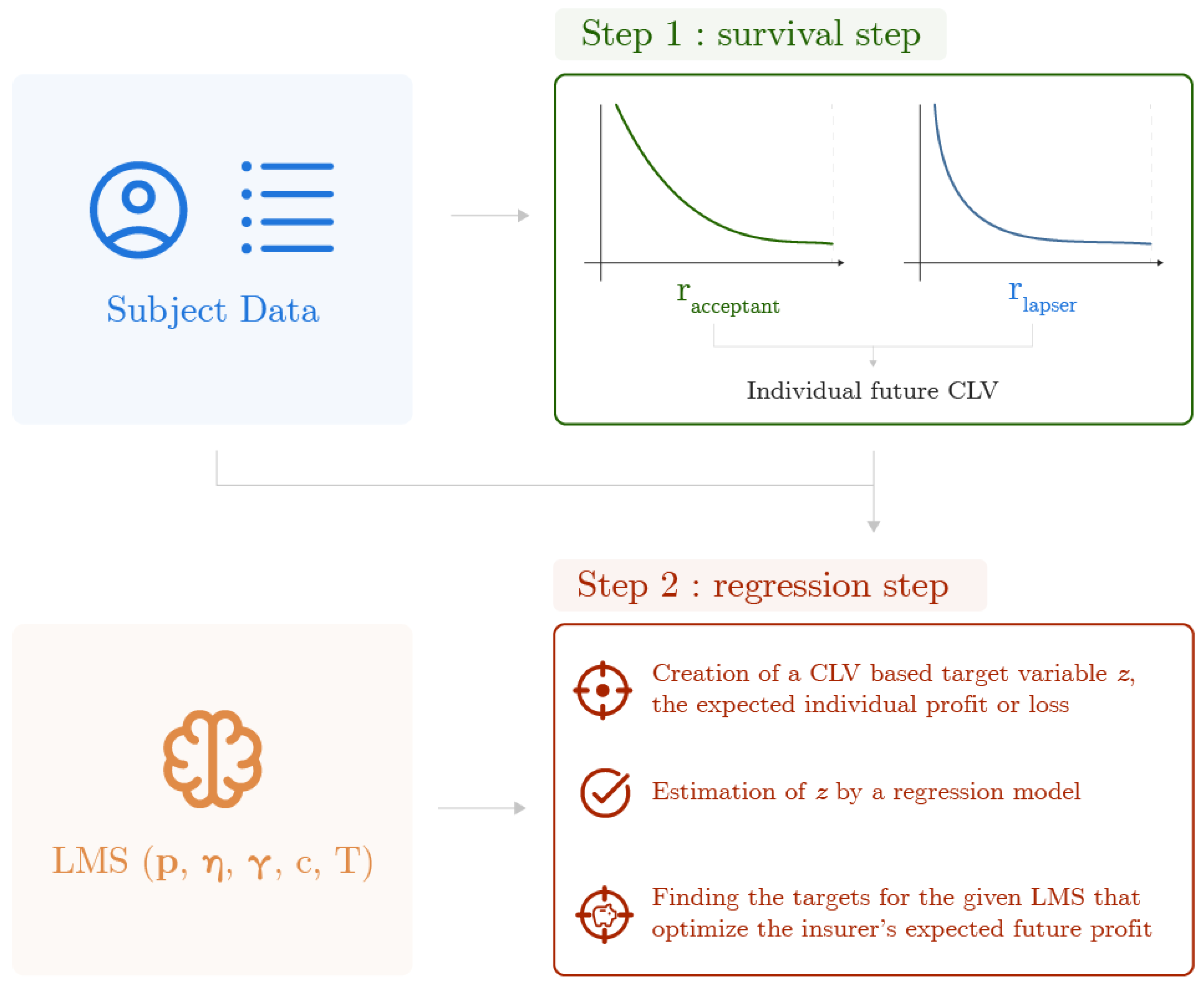
The analysis of a lapse management strategy, as described in [10], then in [7], is a two-step framework. The first step consists of using the insurer’s data to train survival models and predict yearly retention probabilities for any subject in the portfolio: we will refer to it as the survival step. The retention probabilities are used to compute an individual CLV-based estimation of the profit generated from targeting any policyholder. This estimation is eventually used as a response variable to fit a model predicting which kind of subject is likely to generate profit for the insurer: we will refer to it as the regression step. As in [11] or [12], the goal of such a CLV-based methodology is not only to model the lapse behaviour but rather to select which policyholder is worth targeting with a given retention strategy to generate an optimised profit for the insurer. This existing framework relies on the analysis of the time-to-death and time-to-lapse that can be updated regularly with new information from the policies. It is summarised in Figure 1.

At least three limitations of that framework can be addressed. First, it does not consider that an acceptant can lapse in the future, which is at best a very optimistic assumption, and at worst a great oversimplification. Secondly, it does not give any information on whether the timing of the retention campaign is optimal or not. Thirdly, it does not allow tightening the criteria on which the targeting of each policyholder is decided, depending on the risk the insurer is willing to take on the uncertainty of the predictions. This work addresses these limitations.

Throughout the lifetime of such insurance policies, a series of significant time-dependent events shape the interactions between policyholders and insurers. Firstly, premium payments play a pivotal role in sustaining the policy: these payments are highly flexible, allowing policyholders to choose their amount and frequency, thus they can be adjusted according to the policyholder’s financial circumstances and preferences. Additionally, policyholders may decide to reduce their coverage by withdrawing a portion of their policy. We refer to these events as partial lapses: they involve a voluntary decrease in the face amount of the policy, enabling policyholders to adjust their coverage to better align with their changing needs. Such flexibility caters to policyholders’ evolving financial situations and offers them greater control over their insurance plans. Over the policy’s lifetime, other financial operations can occur, such as the payment of interest or profit sharing to the policyholder, and the payment of fees to the insurer. Insurance companies’ information systems are usually designed to keep track of those operations at the policy level, thus actuaries and life insurers often have access to the complete history of their policyholders, as the information system is updated in real-time.

In certain instances, a policyholder may choose to lapse their insurance policy entirely. Complete policy lapse typically occurs when the policyholder decides to terminate their policy and receives a surrender value, which represents the accumulated value of the premiums paid, adjusted for fees, expenses, and potential surrender charges. Moreover, the occurrence of a policyholder’s death also terminates the policy and triggers the payment of the policy’s value, often referred to as the death benefit or claim, to the designated beneficiaries.

In the context of our research, a policy can only terminate with a complete lapse or the death of the policyholder, which will be considered as competing risks in the following developments. If none of these events have happened to a policy, it is still active. The cumulated sum of all the financial flows occurring during one’s policy timeline, including premiums, claims, fees, interests, profit-sharing, and lapses, is commonly known as the face amount of the policy. This face amount represents the total value of the policy over its duration and serves as a measure of the policy’s coverage and financial benefits. By comprehensively understanding and analysing these events and their impact on the face amount of a life insurance policy, insurers can effectively develop lapse management strategies that align with policyholders’ preferences and financial goals. Through our research, we aim to shed light on these dynamics and provide insights to optimise the design of such strategies, ultimately enhancing customer retention and overall portfolio performance in the life insurance industry.

In practice, actuaries often have access to the complete trajectories of every policy and it seems that not using them in models is ignoring a significant part of the available information. A data structure where time-varying covariates are measured at different time points is called longitudinal and individual policyholders’ timelines, which can be illustrated as in Figure 2. The dynamical aspects of covariates have an impact on the performance of lapse prediction models, and [13] concludes in favour of the development of dynamic churn models. They showed how the predictive performance of different types of churn prediction models in the insurance market decays quickly over time: this conclusion arguably applies to life insurers and, in the case of lapse management strategy, we argue that using the complete longitudinal trajectories of every individual is also justified. Firstly, a change in financial behaviour—recent and frequent withdrawals for instance—can be an informative lapse predictor. As an illustration of this point, we can imagine making predictions for two individuals with the same characteristics at the time of study but completely different past longitudinal trajectories: one is consistently paying premiums, for instance, whereas the other stopped all payments for months and has been withdrawing part of their face amount lately. A prediction model ignoring longitudinal information would produce the same lapse prediction for both individuals. Conversely, an appropriate model, trained on longitudinal data is likely to seize the differences between the individuals over time and provide different predictions for the future. Secondly, a longitudinal lapse management framework allows for dynamic predictions with new information. It proves to be insightful in terms of decision-making for the insurer, as it shows how a change in the policy induces a change in the lapse behaviour. Eventually, the existing lapse management strategy approaches can only provide the insurer with information on whether targeting a given individual now is expected to yield profit, not on whether the timing of targeting is optimal. A longitudinal framework can help answer that last question.

In this paper, our goal is to account for the time-varying aspect of this problem in both steps of that framework. Firstly, we take advantage of the information contained in the historical data from the portfolio and obtain more accurate predictions for ${\mathit{r}}^{\left(i\right)}$ and thus ${}^{F}CL{V}^{\left(i\right)}$: that is a gain of precision on the survival step. Secondly, we evaluate the expected individual retention gains over time to derive the optimal timing to offer the incentive: that is a gain of flexibility and expected profit on the regression step. For that purpose, we introduce tree-based models, which are, to the best of our knowledge, yet to be explored in the actuarial literature. Those models, such as left-truncated and right-censored (LTRC) survival trees and LTRC forests by [14,15] or mixed-effect tree-based regression models (see [16,17,18,19]) are considered state-of-the-art and have yet to be exploited in the actuarial literature. We propose an application of that framework with data-driven tree-based models but other types of models exist and could fit in this framework (see Appendix A).

This extension is not trivial, as time-dependent features and time-dependent response variables are difficult to implement in parametric or tree-based models. Indeed, conventional statistical or machine learning models do not readily accommodate time-varying features. This is the case for most tree-based models as they assume that records are independently distributed. Of course, this is unrealistic as observations of any given individual are highly correlated. Moreover, time-varying features can generate bias if not dealt with carefully (see [20] for instance). The use of longitudinal data is already a well-studied topic (see [21]), with rare examples within the actuarial literature (see [22] for instance) and, to the best of our knowledge, only a few actuarial uses of time-varying survival trees or mixed-effect tree-based models have been tried or suggested (see [23], [24] or [25]) and no longitudinal lapse analysis framework based on CLV has been described.

In summary, this work presents a longitudinal lapse analysis framework with time-varying covariates and target variables. This framework accepts competing risks and relies on tree-based machine learning models. This work focuses on a lapse management strategy and retention targeting for life insurers and extends the existing lapse management framework proposed in [7,10]. It defers from the latter by taking advantage of time-varying features, introducing different tree-based models to the lapse management literature, including the possibility for an acceptant to lapse in the future, yielding insights regarding individual targeting times, and adding the possibility to adjust the level of risk, which the insurer is willing to take in a retention campaign. The rest of this paper is structured as follows. We describe the specifics of longitudinal analysis and a new longitudinal and time-dynamic lapse management framework, which is the main contribution of this work in Section 2. This section also includes a brief description of models that can fit in this framework. In Section 3, we show a concrete application of our framework on a real-world life insurance portfolio with a discussion of our methodology and results. Eventually, Section 4 concludes this paper.

Remark 1.

While our primary focus is on the theoretical underpinnings, it is crucial to note that the LMS is adaptable and can be operationalised and adapted in different cultural environments, acknowledging the diversity of social factors that influence actuarial studies.

2. Longitudinal Framework

2.1. Preliminaries on Time-Varying Covariates and Longitudinal Notations

We aim to enrich the existing lapse management frameworks (see Definition 1) with time-varying covariates. To do so, we decide to adapt LMS methods to longitudinal analysis. To be clear on what we mean by time-varying covariates or longitudinal data, let us introduce some notations. This section borrows notations from the existing literature, including [26] or [15], for instance. Let us assume a very general setting where we want to build a dataset $\mathcal{D}$, encompassing the information of N individuals from which features are repeatedly measured over time. These covariates may come in many forms, some of them are time-varying, and others are time-invariant. We denote $p_{tv}$, $p_{ti}$, the number of covariates in those respective categories, with $p=p_{tv}+p_{ti}$, the total number of covariates. At time t, the covariates matrix is $\mathit{X}\left(t\right)=\left(x_1,x_2,\cdots ,x_{p_{ti}},x_{p_{ti}+1}\left(t\right),\dots ,x_p\left(t\right)\right)$. In order to simplify the notations, we write $\mathit{X}\left(t\right)=\left(x_1\left(t\right),x_2\left(t\right),\dots ,x_p\left(t\right)\right)$ with $x_k\left(t\right)=x_k$, $\forall t$ and $\forall k\in [1,\cdots ,p_{ti}]$.

These covariates are available for the N individuals, or subjects, which are observed at discrete time points. Subject i has been observed $n^{\left(i\right)}$ times, at $t_j^{\left(i\right)},j=0,1,\dots ,n^{\left(i\right)}-1$. In our life insurance context, $t_0^{\left(i\right)}$ represents the first measurement of the covariates, i.e., the subscription and times $t_j^{\left(i\right)},j=1,2,\dots ,n^{\left(i\right)}-1$ are the movement dates, i.e., times at which a change in the policy has been recorded. If $t_0^{\left(i\right)}\ne 0$, this means that the baseline information at subscription is missing and the observation is left-truncated. A given subject i, at time $t_j^{\left(i\right)}$ has a vector of covariates denoted ${\mathit{x}}_j^{\left(i\right)}=\left(x_{j,1}^{\left(i\right)},\dots ,x_{j,p}^{\left(i\right)}\right)$ and generally, has a matrix of covariates denoted

$${\mathit{X}}^{\left(\mathit{i}\right)}=\left(\begin{array}{ccc}{x}_{0,1}^{\left(i\right)}& \cdots & x_{0,p}^{\left(i\right)}\\ ⋮& \ddots & ⋮\\ x_{n^{\left(i\right)}-1,1}^{\left(i\right)}& \cdots & x_{n^{\left(i\right)}-1,p}^{\left(i\right)}\end{array}\right)$$

(4)

As stated in Definition 1, the probability of still having an active policy at time t depends on the policyholder’s risk profile. Acceptants are only at risk for death, whereas lapsers are at risk for both lapse and death, and we consider the event of interest to be death and the end of the policy (whatever the cause). Regardless of our outcome of interest, we study the time to an event ending the policy, thus we use the classical survival notations: subject i will eventually experience the event at time $T_{*}^{\left(i\right)}$ and they are no longer observed after censoring time $C^{\left(i\right)}$. We let $T^{\left(i\right)}$ denote the observed event time for subject i, defined as $T^{\left(i\right)}=t_{n^{\left(i\right)}}^{\left(i\right)}=min\left(T_{*}^{\left(i\right)},C^{\left(i\right)}\right)$.

The notations regarding the time dynamics of our data are now clear, so we can structure this information in a longitudinal dataset. To do so, we assume that the time-varying features take constant values between two consecutive observations, that is,

$${\mathit{x}}^{\left(i\right)}\left(t\right)={\mathit{x}}_j^{\left(i\right)},t\in \left[t_j^{\left(i\right)},t_{j+1}^{\left(i\right)}\right),j=0,1,\dots ,n^{\left(i\right)}-1.$$

This assumption is perfectly consistent in an actuarial context where time-varying covariates, such as financial flows, are immediately updated. Any covariate update leads to a new observation and all variables are constant between two consecutive observations. The only limit of this assumption is that updating the insurer’s database usually takes some time and proves to be unrealistic if a policy change has been reported but not yet processed in the information system. An insurance policy at any time point is either active or ended. Moreover, it can only end in two ways: the policyholder either lapses her policy or dies. Thus, we define three event indicators. ${\Delta }^{\left(i\right)}$ is the event indicator, defined at the subject level; it denotes whether individual $\left(i\right)$ has experienced an event (and which one) before censoring time,

$${\Delta }^{\left(i\right)}=\left\{\begin{array}{cc}0\hfill & \mathrm{if}{T}_{*}^{\left(i\right)}>C^{\left(i\right)}\hfill \\ 1\hfill & \mathrm{if}{T}_{*}^{\left(i\right)}\le C^{\left(i\right)}\mathrm{and}\mathrm{EVENT}=\mathrm{lapse}\hfill \\ 2\hfill & \mathrm{if}{T}_{*}^{\left(i\right)}\le C^{\left(i\right)}\mathrm{and}\mathrm{EVENT}=\mathrm{death}.\hfill \end{array}\right.$$

(5)

We also introduce ${\delta }^{\left(i\right)}\left(t\right)$, the event indicator defined at the observation level, it denotes whether individual $\left(i\right)$ has experienced an event (and which one) by time t:

$${\delta }^{\left(i\right)}\left(t\right)={\Delta }^{\left(i\right)}·\mathbb{I}\left\{t\ge T^{\left(i\right)}\right\}.$$

(6)

At the time $t=T_{*}^{\left(i\right)}$, the true event has occurred and we define the ultimate event indicator as

$${\Delta }_{*}^{\left(i\right)}=\left\{\begin{array}{cc}1\hfill & \mathrm{if}\mathrm{EVENT}=\mathrm{lapse}\mathrm{at}\mathrm{time}{T}_{*}^{\left(i\right)}\hfill \\ 2\hfill & \mathrm{if}\mathrm{EVENT}=\mathrm{death}\mathrm{at}\mathrm{time}{T}_{*}^{\left(i\right)}.\hfill \end{array}\right.$$

(7)

It is constant over the observations for a given subject and represents the final value of ${\Delta }^{\left(i\right)}$ when the subject’s policy eventually ends. It can be either equal to 1 or 2. For a subject with an active policy at the censoring time, the value of ${\Delta }_{*}^{\left(i\right)}$ is unknown.

Eventually, let ${\mathcal{X}}^{\left(i\right)}\left(t\right)$ denote the covariate individual information up to time t, and we define ${\pi }_{*}^{\left(i\right)}$ as the probability that the policy will eventually end with lapse (in this framework, our suggestion to estimate ${\pi }_{*}^{\left(i\right)}$ can be found in Appendix C), given all available information at observation time $T^{\left(i\right)}$. Mathematically speaking, we have

$${\displaystyle {\pi }_{*}^{\left(i\right)}=P({\Delta }_{*}^{\left(i\right)}=1|{\mathcal{X}}^{\left(i\right)}\left(T^{\left(i\right)}\right)).}$$

(8)

We can now build $\mathcal{D}$, a longitudinal dataset encompassing the complete past information of all N subjects. For a given subject i, covariates are stored in rows, one row per observation window $[t_j^{\left(i\right)},t_{j+1}^{\left(i\right)})$. Each row contains the unique $\left(t_j^{\left(i\right)},t_{j+1}^{\left(i\right)},{\delta }^{\left(i\right)}\left(t_j^{\left(i\right)}\right),{\mathit{x}}_j^{\left(i\right)}\right)$ element and is completed by the subject unique identifier i and their event indicator ${\Delta }^{\left(i\right)}$: each row is called an observation. It is critical to include all those elements in the longitudinal dataset as all columns are inputs of longitudinal models used for the survival step. Any observation only corresponds to one subject and, conversely, any subject can be linked to a set of $n^{\left(i\right)}$ observations. We build $\mathcal{D}$ as the collection of all observations structured longitudinally:

$$\mathcal{D}={\left\{\left(i,{\left\{t_j^{\left(i\right)},t_{j+1}^{\left(i\right)},{\mathit{x}}_j^{\left(i\right)},{\delta }^{\left(i\right)}\left(t_j^{\left(i\right)}\right)\right\}}_{j=0}^{n^{\left(i\right)}-1},{\Delta }^{\left(i\right)}\right)\right\}}_{i=1}^N,$$

or, if displayed in a table, as in

Table 1. A longitudinal dataset, in all generality.

ID	Time Window Start	Time Window End	Covariate 1	…	Covariate p	Observation Event Indicator	Subject Event Indicator
1	$t_0^{\left(1\right)}$	$t_1^{\left(1\right)}$	$x_{0,1}^{\left(1\right)}$	…	$x_{0,p}^{\left(1\right)}$	${\delta }^{\left(1\right)}\left(t_0^{\left(1\right)}\right)$	${\Delta }^1$
1	$t_1^{\left(1\right)}$	$t_2^{\left(1\right)}$	$x_{1,1}^{\left(1\right)}$	…	$x_{1,p}^{\left(1\right)}$	${\delta }^{\left(1\right)}\left(t_1^{\left(1\right)}\right)$	${\Delta }^1$
1	$t_2^{\left(1\right)}$	$t_3^{\left(1\right)}$	$x_{2,1}^{\left(1\right)}$	…	$x_{2,p}^{\left(1\right)}$	${\delta }^{\left(1\right)}\left(t_2^{\left(1\right)}\right)$	${\Delta }^1$
1	$t_3^{\left(1\right)}$	$C^{\left(1\right)}$	$x_{3,1}^{\left(1\right)}$	…	$x_{3,p}^{\left(1\right)}$	${\delta }^{\left(1\right)}\left(t_3^{\left(1\right)}\right)$	${\Delta }^1$
2	$t_0^{\left(2\right)}$	$t_1^{\left(2\right)}$	$x_{0,1}^{\left(2\right)}$	…	$x_{0,p}^{\left(2\right)}$	${\delta }^{\left(2\right)}\left(t_0^{\left(2\right)}\right)$	${\Delta }^2$
3	$t_0^{\left(3\right)}$	$t_1^{\left(3\right)}$	$x_{0,1}^{\left(3\right)}$	…	$x_{0,p}^{\left(3\right)}$	${\delta }^{\left(3\right)}\left(t_0^{\left(3\right)}\right)$	${\Delta }^3$
3	$t_1^{\left(3\right)}$	$t_2^{\left(3\right)}$	$x_{1,1}^{\left(3\right)}$	…	$x_{1,p}^{\left(3\right)}$	${\delta }^{\left(3\right)}\left(t_1^{\left(3\right)}\right)$	${\Delta }^3$
3	$t_2^{\left(3\right)}$	$t_3^{\left(3\right)}$	$x_{2,1}^{\left(3\right)}$	…	$x_{2,p}^{\left(3\right)}$	${\delta }^{\left(3\right)}\left(t_2^{\left(3\right)}\right)$	${\Delta }^3$
…	…	…	…	…	…	…	…

.

Table 1 precisely illustrates what we call a longitudinal dataset, and a real-world example of such a dataset can be found in Section 3, Table 3. Adapting a lapse management strategy framework to a longitudinal setting means we take such a dataset as input and produce enriched predictions of the individual retention probabilities in the survival step, but also of individual profit or loss estimated in the regression step.

As in the original source and for confidentiality reasons, the exact specificities of the studied products, as well as the proportions between “Euro fund” and equity-linked investments made by the policyholders will not be detailed, nor will their impact be analysed within this article.

2.2. LMS Longitudinal Framework

We adopt [7]’s framework and suggest some modifications and improvements to adapt it to longitudinally structured data. Instead of a top-down approach that consists of estimating the individual contributions to the insurer’s profit from a global measure of the portfolio value, we suggest a bottom-up approach and directly evaluate the former and then derive the latter. Thus, we define the control future value of the policy, ${}^{F}C{V}^{\left(i\right)}(t,\cdots )$, which represents the expected T-year individual profit or loss generated by the subject i, after time t:

$$\begin{array}{cc}\hfill {}^{F}C{V}^{\left(i\right)}(t,\mathit{p},\eta ,\gamma ,c,T)=& {}^{F}CL{V}^{\left(i\right)}\left(t,{\mathit{p}}^{\left(\mathit{i}\right)},{\mathit{F}}^{\left(\mathit{i}\right)},{\mathit{r}}_{\mathrm{acceptant}}^{\left(i\right)},\mathit{d},T\right)·(1-{\pi }_{*}^{\left(i\right)})\hfill \\ \hfill & +{}^{F}CL{V}^{\left(i\right)}\left(t,{\mathit{p}}^{\left(\mathit{i}\right)},{\mathit{F}}^{\left(\mathit{i}\right)},{\mathit{r}}_{\mathrm{lapser}}^{\left(i\right)},\mathit{d},T\right)·{\pi }_{*}^{\left(i\right)}.\hfill \end{array}$$

(9)

In other words, it simply represents an individual expected future CLV, if no lapse management is carried out. It highly depends on the probability for the policyholder to be a lapser.

Let us consider an LMS, let ${⊚}^{\left(i\right)}\left(t\right)$ be the individual target vector indicator, designating if subject i is to be targeted at any time t. Our framework aims to find the optimal list of policyholders to target, $\mathcal{T}\left(t\right)=\{i\mid {⊚}^{\left(i\right)}\left(t\right)=1\}$ that maximises the expected profit for the insurer. To evaluate the profit or loss generated by an LMS, we must compare the expected profit obtained if no LMS was applied, with the expected profit generated by the lapse-managed portfolio. The former is given by Equation (9), and to obtain the latter, we define the lapse-managed observation future value as

$$\begin{array}{cc}\hfill & {}^{F}LM{V}^{\left(i\right)}(t,\mathit{p},\eta ,\gamma ,c,T)=\hfill \\ \hfill & \hspace{1em}\hspace{1em}\left[{}^{F}CL{V}^{\left(i\right)}\left(t,{\mathit{p}}^{\left(\mathit{i}\right)},{\mathit{F}}^{\left(\mathit{i}\right)},{\mathit{r}}_{\mathrm{acceptant}}^{\left(i\right)},\mathit{d},T\right)·(1-{\pi }_{*}^{\left(i\right)})+{}^{F}CL{V}^{\left(i\right)}\left(t,{\mathit{p}}^{\left(\mathit{i}\right)},{\mathit{F}}^{\left(\mathit{i}\right)},{\mathit{r}}_{\mathrm{lapser}}^{\left(i\right)},\mathit{d},T\right)·{\pi }_{*}^{\left(i\right)}\right]·(1-{⊚}^{\left(i\right)}\left(t\right))\hfill \\ \hfill & \hspace{1em} +[{}^{F}CL{V}^{\left(i\right)}\left(t,{\mathit{p}}^{\left(\mathit{i}\right)}-{\eta }^{\left(\mathit{i}\right)},{\mathit{F}}^{\left(\mathit{i}\right)},{\mathit{r}}_{\mathrm{acceptant}}^{\left(i\right)},\mathit{d},T\right)·(1-{\pi }_{*}^{\left(i\right)})+{\gamma }^{\left(i\right)}·{}^{F}CL{V}^{\left(i\right)}\left(t,{\mathit{p}}^{\left(\mathit{i}\right)}-{\eta }^{\left(\mathit{i}\right)},{\mathit{F}}^{\left(\mathit{i}\right)},{\mathit{r}}_{\mathrm{acceptant}}^{\left(i\right)},\mathit{d},T\right)·{\pi }_{*}^{\left(i\right)}\hfill \\ \hfill & \hspace{1em}\hspace{1em}\hspace{1em}+(1-{\gamma }^{\left(i\right)})·{}^{F}CL{V}^{\left(i\right)}\left(t,{\mathit{p}}^{\left(\mathit{i}\right)},{\mathit{F}}^{\left(\mathit{i}\right)},{\mathit{r}}_{\mathrm{lapser}}^{\left(i\right)},\mathit{d},T\right)·{\pi }_{*}^{\left(i\right)}-c]·{⊚}^{\left(i\right)}\left(t\right).\hfill \end{array}$$

(10)

In simple terms, it is equal to the control future value of the policy (given by Equation (9)) when subject i is not targeted, otherwise, it depends on whether they intended to lapse in the first place and, if so, if they accept the incentive $\eta$. If a policyholder that would not have lapsed (with probability $(1-{\pi }_{*}^{\left(i\right)})$) is targeted, they will rationally accept the incentive and generate the future CLV of an acceptant with profitability p − η. Conversely, for a policyholder that would have ultimately lapsed, they either accept the incentive (with probability ${\gamma }^{\left(i\right)}$) and generate the future CLV of an acceptant with profitability p − η, or refuse (with probability $(1-{\gamma }^{\left(i\right)})$) and generate profitability p with the risk profile of a lapser.

It follows that the individual expected retention gain obtained by applying an LMS is the difference between the expected individual CLVs with and without lapse management:

$$R{G}^{\left(i\right)}(t,\mathit{p},\eta ,\gamma ,c,T)={}^F\mathrm{LMV}^{\left(\mathrm{i}\right)}(t,{\mathit{p}}^{\left(\mathit{i}\right)},{\eta }^{\left(\mathit{i}\right)},{\gamma }^{\left(\mathit{i}\right)},c,T)-{}^{F}C{V}^{\left(i\right)}(t,{\mathit{p}}^{\left(\mathit{i}\right)},{\eta }^{\left(\mathit{i}\right)},{\gamma }^{\left(\mathit{i}\right)},c,T).$$

(11)

that can be simplified as

$$\begin{array}{cc}\hfill R{G}^{\left(i\right)}(t,\mathit{p},\eta ,\gamma ,c,T)=& {⊚}^{\left(i\right)}\left(t\right)·\left[{\pi }_{*}^{\left(i\right)}{\gamma }^{\left(i\right)}\right[{}^{F}CL{V}^{\left(i\right)}\left(t,{\mathit{p}}^{\left(\mathit{i}\right)}-{\eta }^{\left(\mathit{i}\right)},{\mathit{F}}^{\left(\mathit{i}\right)},{\mathit{r}}_{\mathrm{acceptant}}^{\left(i\right)},\mathit{d},T\right)\hfill \\ \hfill & \hspace{1em}\hspace{1em}\hspace{1em}\hspace{1em}\hspace{1em}-{}^{F}CL{V}^{\left(i\right)}\left(t,{\mathit{p}}^{\left(\mathit{i}\right)},{\mathit{F}}^{\left(\mathit{i}\right)},{\mathit{r}}_{\mathrm{lapser}}^{\left(i\right)},\mathit{d},T\right)]\hfill \\ \hfill & -(1-{\pi }_{*}^{\left(i\right)})·{}^{F}CL{V}^{\left(i\right)}\left(t,{\eta }^{\left(\mathit{i}\right)},{\mathit{F}}_{\mathit{i}},{\mathit{r}}_{\mathrm{acceptant}},\mathit{d},T\right)]-c·{⊚}^{\left(i\right)}\left(t\right).\hfill \end{array}$$

(12)

An evaluation metric is finally derived to obtain the retention gain, at any observation time, if the policyholder i is targeted. We define $z^{\left(i\right)}\left(t\right)$ as

$$\begin{array}{cc}\hfill z^{\left(i\right)}\left(t\right)& =R{G}^{\left(i\right)}(t,\mathit{p},\eta ,\gamma ,c,T|{⊚}^{\left(i\right)}\left(t\right)=1)\hfill \\ \hfill & =\left[{\pi }_{*}^{\left(i\right)}{\gamma }^{\left(i\right)}\right[{}^{F}CL{V}^{\left(i\right)}\left(t,{\mathit{p}}^{\left(\mathit{i}\right)}-{\eta }^{\left(\mathit{i}\right)},{\mathit{F}}^{\left(\mathit{i}\right)},{\mathit{r}}_{\mathrm{acceptant}}^{\left(i\right)},\mathit{d},T\right)\hfill \\ \hfill & \hspace{1em}\hspace{1em}\hspace{1em} -{}^{F}CL{V}^{\left(i\right)}\left(t,{\mathit{p}}^{\left(\mathit{i}\right)},{\mathit{F}}^{\left(\mathit{i}\right)},{\mathit{r}}_{\mathrm{lapser}}^{\left(i\right)},\mathit{d},T\right)]\hfill \\ \hfill & -(1-{\pi }_{*}^{\left(i\right)})·{}^{F}CL{V}^{\left(i\right)}\left(t,{\eta }^{\left(\mathit{i}\right)},{\mathit{F}}^{\left(\mathit{i}\right)},{\mathit{r}}_{\mathrm{acceptant}}^{\left(i\right)},\mathit{d},T\right)]-c.\hfill \end{array}$$

(13)

In terms of intuition, it shows that if a policyholder that would have lapsed (with probability ${\pi }_{*}^{\left(i\right)}$) is targeted and accepts the incentive (with probability ${\gamma }^{\left(i\right)}$), they generate the future CLV of an acceptant with profitability p − η instead of their initial future CLV with profitability p and the risk profile of a lapser. The gain generated by targeting this policyholder is then the difference between the two. On the other hand, if the policyholder is wrongfully targeted and would not have lapsed (with probability $(1-{\pi }_{*}^{\left(i\right)})$), they rationally accept the incentive which is then lost for the insurer. In any case, the contact cost of c is spent.

From a practical point of view, we can see that the value of $z^{\left(i\right)}\left(t\right)$ depends on parameters that are observed in the portfolio (${\mathit{F}}^{\left(\mathit{i}\right)}$), or assumed by the insurer (${\mathit{p}}^{\left(\mathit{i}\right)},{\eta }^{\left(\mathit{i}\right)},\mathit{d},T$), and that only ${\mathit{r}}_{\mathrm{acceptant}}^{\left(i\right)}$ and ${\mathit{r}}_{\mathrm{lapser}}^{\left(i\right)}$ need to be estimated. This estimation is the survival step mentioned in Section 1. We will show in Section 3.2.1 how to concretely estimate these retention probabilities using time-varying covariates.

Assuming that ${\mathit{z}}^{\left(\mathit{i}\right)}$ has been estimated for every observation in the survival step, we can move forward to the regression step and use ${\mathit{z}}^{\left(\mathit{i}\right)}$ as a target variable in a regression model handling time-varying covariates to predict whether targeting any policyholder will generate profit, given their previous observations if any. We will show in Section 3.3.1 how to concretely obtain ${\widehat{\mathit{z}}}^{\left(\mathit{i}\right)}$ with mixed-effect tree-based models.

With that in mind, we can update Definition 1 and its hypothesis and define our LLMS as follows:

Definition 2

(Longitudinal lapse management strategy (LLMS)). A T-years lapse management strategy is modelled by offering an incentive ${\eta }^{\left(i\right)}$ to subject i if they are targeted. The incentive offered is expressed as a percentage of their face amount at the observation time and is accepted with probability ${\gamma }^{\left(i\right)}$. Contacting the targeted policyholder has a fixed cost of c. Relying on previous implementations of this framework, a targeted subject who accepts the incentive would be considered an “acceptant” who should theoretically never lapse (and thus is only at risk for death), and their probability of being active at year $t\in [0,T]$, given the information available until then, is denoted $r_{\mathit{acceptant}}^{\left(i\right)}(t\mid {\mathcal{X}}^{\left(i\right)}\left(t\right))$. Conversely, a subject who refuses the incentive and prefers to lapse (and thus is at risk for death and lapse) would be considered a “lapser”, and their probability of being active at year t, given the information available until then, is denoted $r_{\mathit{lapser}}^{\left(i\right)}(t\mid {\mathcal{X}}^{\left(i\right)}\left(t\right))$. This article assumes that all PH are not 100% lapsers nor 100% acceptants but rather that their true risk profiles lie in between. Thus, the future profit or loss generated by any policyholder is computed as a weighted sum of CLVs, respectively, calculated with the risk profiles of an “acceptant” and a “lapser”.

Those probabilities are used to derive a dynamical profit-driven measure $z^{\left(i\right)}\left(t\right)$ based on CLV (see Equation (13)). A regression model, allowing for longitudinal data is then used with $z^{\left(i\right)}\left(t\right)$ as a target variable, which allows us to estimate ${\widehat{z}}^{\left(i\right)}\left(t\right)$ for any new observations (new observations of known subjects or observations of new subjects). Denoting the standard error of such a model ${\sigma }_z$ and any confidence parameter α, we define the optimal longitudinal LMS at time t as

$${⊚}_{*}^{\left(i\right)}\left(t\right)=\mathbb{I}\left\{{\widehat{z}}^{\left(i\right)}\left(t\right)>\alpha ·{\sigma }_z\right\}.$$

(14)

This is an indicator variable representing whether it is worth targeting policyholder i at time t, thus, the corresponding list of targeted policyholders is defined as

$$\mathcal{T}\left(t\right)=\left\{i\mid {⊚}_{*}^{\left(i\right)}\left(t\right)=1\right\}.$$

(15)

For any targeted policyholder and any confidence parameter α desired by the insurer, there is a unique future time $t_{*}^{\left(i\right)}\ge T^{\left(i\right)}$ when offering the incentive is optimal, which yields a maximal profit of ${\widehat{z}}_{*}^{\left(i\right)}$. If all policyholders in $\mathcal{T}\left(t\right)$ are targeted at time t, the LLMS generates a profit of

$${\displaystyle RG(t,\mathit{p},\eta ,\gamma ,c,T,\alpha )=\sum _{i\in \mathcal{T}\left(t\right)}{\widehat{z}}^{\left(i\right)}\left(t\right).}$$

(16)

If all policyholders are targeted at the optimal time $t_{*}^{\left(i\right)}\ge t$, the LLMS induces a gain for the life insurer of

$${\displaystyle \stackrel{*}{RG}(t,\mathit{p},\eta ,\gamma ,c,T,\alpha )=\sum _{i\in \mathcal{T}\left(t\right)}\frac{{\widehat{z}}_{*}^{\left(i\right)}}{{\left(1+d_{t_{*}^{\left(i\right)}}\right)}^{\Delta t}},\mathit{with}\Delta t=t_{*}^{\left(i\right)}-t.}$$

(17)

The addition of a confidence parameter $\alpha$ contrasts with previous approaches (see [7,10]). Setting $\alpha =0$ means that the prediction ${\widehat{z}}^{\left(i\right)}\left(t\right)$ is trusted with 100% confidence by the insurer, whereas letting $\alpha$ take higher values ensures that ${\widehat{z}}^{\left(i\right)}\left(t\right)$ is positive with a given confidence interval. Another novelty here is the time dynamic of those results. Not only can we predict whether it is worth targeting a given policyholder, but we can also predict whether there will be some point in the future when targeting them will be more profitable. Predicting the trajectory of $z^{\left(i\right)}\left(t\right)$ at future time points requires projecting the time-varying covariates at those future time points. It can be done by either modelling such covariates individually or setting assumptions. It is trivial for covariates such as age or year but more complex for stochastic covariates such as the face amount. This framework does not aim to answer this question, and we assume in our application that stochastic covariates remain constant and equal to their last observed value. Regardless of the assumptions, the framework allows adding a time dimension to the LMS optimisation and marketing decision-making. It is also worth noting that our developed framework is consistent in the time-invariant case. By design, it is also fully applicable with uncensored observations, or left-truncated ones. That shows our two-step framework’s broad effectiveness and applicability regardless of right-censorship, left-truncation, risk factor, time-varying covariates, or time-varying effects. In that sense, it is a generalised framework for lapse management strategy in life insurance.

Remark 2.

Following the proposed longitudinal methodology, a dynamic targeting decision process is obtained. Nevertheless, no information about the future trajectories of longitudinal covariates can be deduced directly from the framework. Indirectly, one could establish clusters of individuals based on their lapse behaviour and assume that a policyholder in one cluster will behave as the other policyholders in the cluster who have been observed longer. That specific approach is out of the scope of this article and will be left as future work.

The proposed framework requires the projection of every term in the future with assumptions and/or specific modelling approaches: periodical payments and profit sharing can be assumed to remain unchanged, while spontaneous payments, partial lapses, or up-sells and cross-sells can be either ignored or modelled.

Eventually, a projection of every longitudinal covariate along with the response variable could be considered with the use of joint modelling techniques (see [26] for further details), but again, such considerations lie far beyond the scope of this work.

3. Application

3.1. Data

Our framework is inspired by a real-world life insurance dataset used in [7]. It initially contains the most recent information from 248,737 unique policies contracted between 1997 and 2018 and 235,076 unique policyholders. A single row originally represented a unique policy/policyholder pair, identified by a unique ID and denoted as a subject. Due to great computation times, we restrain our application on a 10,000-subjects subset of this original dataset, which preserves key characteristics of the entire population, such as mean seniority (∼13 years), the proportion of policies owned by men (∼57%), and the proportions of lapses and deaths observed in the portfolio (respectively 22% and 17%). More details about the complete dataset, such as a demographic description of the subjects can be found in [7].

The 10,000 rows dataset containing the last available information for the 10,000 selected subjects will be denoted ${\mathcal{D}}^{\mathit{last}}$. Table 2 shows a subset of ${\mathcal{D}}^{\mathit{last}}$ for illustrative purposes.

Table 2. ${\mathcal{D}}^{\mathit{last}}$ random subset.

ID	EVENT	PRODUCT	SEX	SENIORITY	${\mathit{F}}_{\mathit{i}}$	CLAIM	CNTRCTS	AGE	YEAR
25737	1	1	1	17	0.73	0	2	76	2015
117322	1	1	2	10	4.32	0	1	63	2012
1322	0	1	2	20	9.82	0	1	75	2019
37433	2	1	2	14	0.99	−50.49	1	88	2011
23902	0	1	1	20	32.66	−13.12	2	71	2019
219281	0	2	2	8	7.08	0	2	71	2019
160112	0	1	2	15	0.04	0	1	51	2019
53108	2	1	2	12	13.11	−661.92	1	92	2010
166078	1	2	2	5	9.02	0	1	64	2013
139644	0	1	1	16	5.65	−107.59	1	66	2019

Table 2. ${\mathcal{D}}^{\mathit{last}}$ random subset.

ID	EVENT	PRODUCT	SEX	SENIORITY	${\mathit{F}}_{\mathit{i}}$	CLAIM	CNTRCTS	AGE	YEAR
25737	1	1	1	17	0.73	0	2	76	2015
117322	1	1	2	10	4.32	0	1	63	2012
1322	0	1	2	20	9.82	0	1	75	2019
37433	2	1	2	14	0.99	−50.49	1	88	2011
23902	0	1	1	20	32.66	−13.12	2	71	2019
219281	0	2	2	8	7.08	0	2	71	2019
160112	0	1	2	15	0.04	0	1	51	2019
53108	2	1	2	12	13.11	−661.92	1	92	2010
166078	1	2	2	5	9.02	0	1	64	2013
139644	0	1	1	16	5.65	−107.59	1	66	2019

Here, we were able to retrieve the longitudinal history of every subject present in ${\mathcal{D}}^{\mathit{last}}$: this means that for every policy and policyholder, we observe every payment, lapse, fee, profit sharing, or discount rate from the policy subscription to the most updated information to date along with baseline covariates such as gender or age at subscription. For operational reasons, the longitudinal data are measured and reported yearly and organised as follows (but it is worth mentioning that covariates in actuarial datasets are usually updated continuously. In that case, we could build a continuous longitudinal dataset with one observation per policy change, and not one per year. The framework detailed here still applies in the continuous case.):

Table 3. ${\mathcal{D}}^{\mathit{long}}$ random subset.

ID	EVENT	START	END	PRODUCT	SEX	SENIORITY	${\mathit{F}}_{\mathit{i}}$	CLAIM	CNTRCTS	AGE	YEAR
46784	0	0	1	3	2	0	8.38	0	1	66	2013
46784	0	1	2	3	2	1	8.40	0	1	67	2014
46784	0	2	3	3	2	2	8.57	0	1	68	2015
46784	0	3	4	3	2	3	11.90	0	1	69	2016
46784	0	4	5	3	2	4	12.10	0	1	70	2017
46784	0	5	6	3	2	5	12.28	0	1	71	2018
46784	1	6	7	3	2	7	15.06	−15.06	1	72	2019
7825	0	0	1	2	2	0	3.02	0	1	81	2016
7825	0	1	2	2	2	1	3.05	0	1	82	2017
7825	0	2	3	2	2	2	3.10	0	1	83	2018
7825	0	3	5	2	2	5	3.15	0	1	84	2019
264309	0	0	1	3	2	0	2.61	0	1	66	2016
264309	0	1	2	3	2	1	2.64	0	1	67	2017
264309	0	2	3	3	2	2	2.67	0	1	68	2018
264309	0	3	5	3	2	5	3.48	0	1	69	2019

Table 3. ${\mathcal{D}}^{\mathit{long}}$ random subset.

ID	EVENT	START	END	PRODUCT	SEX	SENIORITY	${\mathit{F}}_{\mathit{i}}$	CLAIM	CNTRCTS	AGE	YEAR
46784	0	0	1	3	2	0	8.38	0	1	66	2013
46784	0	1	2	3	2	1	8.40	0	1	67	2014
46784	0	2	3	3	2	2	8.57	0	1	68	2015
46784	0	3	4	3	2	3	11.90	0	1	69	2016
46784	0	4	5	3	2	4	12.10	0	1	70	2017
46784	0	5	6	3	2	5	12.28	0	1	71	2018
46784	1	6	7	3	2	7	15.06	−15.06	1	72	2019
7825	0	0	1	2	2	0	3.02	0	1	81	2016
7825	0	1	2	2	2	1	3.05	0	1	82	2017
7825	0	2	3	2	2	2	3.10	0	1	83	2018
7825	0	3	5	2	2	5	3.15	0	1	84	2019
264309	0	0	1	3	2	0	2.61	0	1	66	2016
264309	0	1	2	3	2	1	2.64	0	1	67	2017
264309	0	2	3	3	2	2	2.67	0	1	68	2018
264309	0	3	5	3	2	5	3.48	0	1	69	2019

Moreover, all the covariates describing financial flows are observed as cumulated over the years. As an example, let us assume that a subject subscribed in the year 2000: their payment variable for the year 2000 observation contains the sum of all payments that occurred in that year, their payment variable for the year 2001 contains the sum of all payments that occurred up to the year 2001 included (hence, 2000 and 2001), and so on for the years after. This longitudinal dataset will be denoted ${\mathcal{D}}^{\mathit{long}}$. It contains 126,865 observations, in other words, almost 13 for each subject. Subsets of this specific longitudinal dataset are studied in [27].

For privacy reasons, all the data, statistics, product names, and perimeters presented in this paper have been either anonymised or modified. For instance, information about the policyholders’ age and face amount were modified. All analyses, discussions, and conclusions remain unchanged.

3.2. Application: Survival Step

3.2.1. Survival Analysis with Time-Varying Covariates

The survival step, described in Section 2 requires survival tree-based models that can handle longitudinal time-varying covariates. Most survival tree-based models are analogous to regular tree-based models: survival trees work similarly to regular decision trees, creating partitions of the covariate space. What differentiates them is the splitting criterion that splits by maximising the difference between two considered child nodes. Typically, at each node and for each split considered, a log-rank test is used to test the null hypothesis that there is no difference between the child nodes in the probability of an event at any time. The split that minimises the p-value is then selected. By extension, a random survival forest is a random forest of survival trees.

As regression and classification trees, most survival trees are unable to deal with time-varying and longitudinal covariates. Indeed, let $x_1\left(t\right)$ be a numerical time-varying covariate. For a single tree, the splitting rule should be able to split subjects into two child nodes at each node. It would then be a rule of the form “$x_1\le s$”. A subject for which this rule is true $\forall t$ will go in one child node without any ambiguity. On the other hand, the general case where the rule is true for some periods but false for anywhere else is unclear and needs to be addressed. Note that the same reasoning can be applied to categorical time-varying covariates as well. A simple idea is that the subject’s observations in periods where the splitting rule is true would go to the left node, and the other would go to the right node, thus dividing one subject into several pseudo-subjects. With a longitudinal dataset, that method just implies considering all rows as independent, which creates correlated right-censored and left-truncated (LTRC) observations that need special treatment. In such models, any individual can be spread in many different tree leaves—even if, at any fixed time, any individual will have a single observation that will fall into one unique leaf. Ref. [14] proposed a model based on those ideas: they allowed subjects to be divided into pseudo-subjects and adjusted the log-rank test in the splitting procedure to accommodate for left truncation and ensure that the independence implicit assumption does not lead to biased results (see [14] for details on that point.).

LTRC trees and forests yield an estimate of the survival function:

$$\widehat{S}\left(t\mid {\mathcal{X}}^{\left(i\right)}\left(t\right)\right)=P(T^{\left(i\right)}>t\mid {\mathcal{X}}^{\left(i\right)}\left(t\right)),$$

that can directly be used to evaluate the conditional incidence functions for competing risks (see Appendix D). Bagging models of such trees then emerged (see [15]), with the usual prediction advantages and interpretability drawbacks of such bagging techniques (both methods have been implemented in the R packages LTRCtrees v1.1.1 and LTRCforests, and are considered state-of-the-art methods for tree-based survival analysis with time-varying covariates). To evaluate the survival models’ performance, we chose to use the time-dependent Brier score (td-BS), integrated Brier score (td-IBS), Brier skill score (td-BSS), and integrated Brier skill score (td-IBSS) for longitudinal data (as in [15]). More details about these metrics can be found in Appendix D.3.

3.2.2. Comparison Settings

We propose here a comparison framework to measure the benefits of including the historical data in ${\mathcal{D}}^{\mathit{long}}$, compared to using ${\mathcal{D}}^{\mathit{last}}$. The matrices $r_{lapser}$ and $r_{acceptant}$ are estimated with the algorithms LTRCRRF and LTRCCIF from the R package LTRCforests (In the following sections, we consider LTRCRRF and LTRCCIF: LTRC forests, respectively, based on regular CART and conditional inference survival tree algorithms. More insights about those models can be found in the references detailed in Section 3.2.1.). To assess the advantages of that longitudinal model, we compare its results with those obtained with the gradient boosting survival model (GBSM) as it proved to be a high-performing non-longitudinal model on that dataset (see [7]). With $T^{\left(i\right)}$, the “any event” time for subject i (that is the censoring time for active policies and the termination time, whatever the cause, for all others), $r_{lapser}$ and $r_{acceptant}$ are estimated from the respective survival functions

$${\widehat{S}}_{\mathrm{lapser}}\left(t\mid {\mathcal{X}}^{\left(i\right)}\left(t\right)\right)=P(T^{\left(i\right)}>t\mid {\mathcal{X}}^{\left(i\right)}\left(t\right)),$$

$${\widehat{S}}_{\mathrm{acceptant}}\left(t\mid {\mathcal{X}}^{\left(i\right)}\left(t\right)\right)=P(T^{\left(i\right)}>t,\mathrm{EVENT}=\mathrm{death}\mid {\mathcal{X}}^{\left(i\right)}\left(t\right)),$$

with observations that ended with lapse considered as censored in the estimation of ${\widehat{S}}_{\mathrm{acceptant}}$.

We want to compare the performance of all models trained with and without longitudinal data but also compare them on different tasks. Typically, predictions on ${\mathcal{D}}^{\mathit{last}}$ and ${\mathcal{D}}^{\mathit{long}}$ do not answer the same questions. The former aims at predicting the last observation of the target variable, and the latter aims at predicting its value at any given point in time. Depending on whether the model has been trained on longitudinal data or only on the most recent observation and with different prediction goals, this naturally designs the following four settings that answer four prediction problems:

(a)

Models are trained on ${\mathcal{D}}_{train}^{last}$ and evaluated on predictions from ${\mathcal{D}}_{test}^{last}$;

(b)

Models are trained on ${\mathcal{D}}_{train}^{long}$ and evaluated on predictions from ${\mathcal{D}}_{test}^{last}$;

(c)

Models are trained on ${\mathcal{D}}_{train}^{last}$ and evaluated on predictions from ${\mathcal{D}}_{test}^{long}$;

(d)

Models are trained on ${\mathcal{D}}_{train}^{long}$ and evaluated on predictions from ${\mathcal{D}}_{test}^{long}$.

Setting (a) is the classical setting, where any subject has only one measurement, and the prediction task is also to predict a variable at one given time point. Conversely, setting (d) represents the longitudinal setting, where models are trained with longitudinal time-varying covariates and where the prediction task aims at retrieving the value of a target variable at any given time point during a subject’s lifetime. Setting (c) is not insightful as a model trained on aggregated data cannot retrieve longitudinal information and is expected to perform poorly by design. Intermediate setting (b) is also insightful as it can be used to highlight the added value of the information contained in longitudinal data when training a model. The comparison is made on a time-varying survival evaluation metric: the time-dependent Brier skill score (td-BSS) for longitudinal data (see Appendix D.3).

3.2.3. Results

First of all, to assess the superiority of longitudinal models in a longitudinal context, we need to compare all our considered models in the classical aggregated setting: with training and testing phases on subsets of ${\mathcal{D}}^{\mathit{last}}$. We can see that in this non-longitudinal setting, GBSM and LTRC models (LTRCRRF and LTRCCIF) are close in terms of BSS. Figure 3 displays the td-BSS on the y-axis, for which a value of 0 means that the score for the predictions is merely as good as that of a naive prediction (in our application, the empirical estimate of the survival function has been chosen as the naive prediction) and a value of 1 is the best score possible. BSSs are computed for every time point, meaning that we can observe and compare the performance of models in estimating retention probabilities for low-seniority policies or high-seniority ones independently.

The IBSS, the mean of BSSs over all time points (see Appendix D.3), indicates that LTRCRRF performs slightly better than LTRCCIF, hence we will drop LTRCCIF for the rest of this application. In real-world scenarios, the inherent complexity of the true survival distribution might include time-varying covariates and time-varying effects. The cross-validated Brier scores and Brier score skills graphs (see the Monte-Carlo cross-validation procedure described in Appendix B) can potentially lead decision makers to choose different survival estimations at different time points and not a unique choice of method for all time points.

In contrast, the difference between those models is evident and significant whenever they are trained on longitudinal data. Figure 4 and Figure 5 below show the difference in terms of BSS over time in prediction settings (b) and (d).

The conclusion regarding prediction richness contained in longitudinal data and accuracy benefits from using dedicated longitudinal methods is clear. Longitudinal models perform significantly better, and GBSM brings minor improvement over naive models.

In the end, we select LTRCRRF for estimating the retention probabilities in the survival step as it shows to be the best model when trained on longitudinal data.

It is to be noted that the results of that modelling approach in terms of global retention gain (Equation (16)) are not necessarily better than the results obtained without the use of longitudinal data in the estimation of $r_{lapser}$ and $r_{acceptant}$. In other words, a better performance of the model used in the survival step does not lead to an increase in the insurer’s expected profit, for a given LMS but to a more realistic estimation of it as they model the CLV more accurately.

With that, we determine $r_{lapser}$ and $r_{acceptant}$, the conditional retention probabilities for every observation to derive the trajectory of the observed individual CLV, RG, and eventually $z^{\left(i\right)}\left(t\right)$ (see Equation (13)). The latter can then be used as a longitudinal target variable in a regression model: this constitutes the regression step, introduced in Section 1 and detailed within this application in the next Section.

Another advantage of using longitudinal data for survival analysis is that it helps study how a given subject’s retention probabilities are updated with time. In Figure 6, we take the example of a randomly selected subject and plot their retention probability at every observation time. The further in time the observation is, the more transparent the survival curve is. The individual retention curves are updated as new measurements are available.

3.3. Application: Regression Step

3.3.1. Regression Analysis with Time-Varying Covariates

The regression step of the framework introduced in Section 2.2 requires using a regression model allowing for longitudinal data to produce an estimate of $z^{\left(i\right)}\left(t\right)$. We chose to use mixed-effect tree-based models (METBM). First of all, a mixed-effect model is designed to work on clustered data in general, including longitudinal data (see [28]). Refs. [16,17,18,19] describe a procedure to fit a mixed effect model using tree-based models through an iterative two-step process (the algorithms corresponding to their respective work are available in the R packages REEMtree and LongituRF, the R function “REEMctree” and the Python library MERF.). Mixed-effect tree-based algorithms are designed to take clustered data as input. By considering subjects as clusters, they can grasp the dependence structure within the different observations of a single subject and can be used for longitudinal analysis (see [28]).

The underlying idea behind mixed-effect tree-based algorithms is to assume a mixed model for the longitudinal outcome and estimate the random effect parameters with a tree-based model. Such approaches estimate the random effects of a mixed model in the first step and then construct a regression tree with the fixed-effect covariates on the original outcome, excluding the estimated random effect. The idea is to repeat these two steps: the model parameters and the random effects are estimated iteratively until convergence, similar to the two-step well-known EM optimisation procedure. Suppose that we have $p_f$ covariates with a fixed effect and $p_s$ covariates with a random effect. Initially, a parametric linear mixed-effect model is given by

$${\mathit{z}}^{\left(\mathit{i}\right)}=F^{\left(i\right)\top }\beta +S^{\left(i\right)\top }{\mathit{b}}^{\left(\mathit{i}\right)}+{ϵ}^{\left(\mathit{i}\right)}.$$

(18)

where ${\mathit{z}}^{\left(\mathit{i}\right)}$ is the $n^{\left(i\right)}\times 1$ longitudinal vector outcome of subject i, $\beta$ is the $p_f\times 1$ vector of the fixed effect coefficients and $F^{\left(i\right)}$ is the $n^{\left(i\right)}\times p_f$ design matrix of the covariates with a fixed effect. The quantity ${\mathit{b}}^{\left(\mathit{i}\right)}$ is the $p_s\times 1$ vector of random effects, and $S^{\left(i\right)}$ is the $n^{\left(i\right)}\times p_s$ design matrix of the covariates with a subject-specific effect. By construction, $F^{\left(i\right)}$ and $S^{\left(i\right)}$ are subdivisions of the covariate space. The error term ${ϵ}^{\left(\mathit{i}\right)}$ is the $n^{\left(i\right)}\times 1$ vector of residuals, assumed to come from a normal distribution with mean 0 and variance ${\sigma }^2$, and we assume ${\mathit{b}}^{\left(\mathit{i}\right)}\sim \mathcal{N}(0,D)$, ${ϵ}^{\left(\mathit{i}\right)}\sim \mathcal{N}(0,{\sigma }^2·{\mathbb{I}}_{n^{\left(i\right)}})$. Eventually, D is the $p_s\times p_s$ variance–covariance matrix for the random effects.

To model a longitudinal outcome with non-linear fixed effects, a tree-based model is included in Equation (18), as follows:

$${\mathit{z}}^{\left(\mathit{i}\right)}=f\left(F^{\left(i\right)}\right)+S^{{\left(i\right)}^{\top }}{\mathit{b}}^{\left(\mathit{i}\right)}+{ϵ}^{\left(\mathit{i}\right)}.$$

(19)

Here, the linear structure of the fixed effect part of the model is generalised: the fixed effects are described by a function of the fixed-effect covariates f, which is the part that a tree-based model will estimate. In MERT (see [29]), the tree-based model is a single regression tree, in MERF (see [17]), it is a random forest, whereas in RE-EM (see [16,18]), it can be both. A general algorithm for such mixed-effect tree-based models can be described in Algorithm 1.

Algorithm 1: Mixed-effect tree-based model pseudo-code.

1: Input: $\mathcal{D}$, a longitudinal dataset with an outcome ${\mathit{z}}^{\left(\mathit{i}\right)}$, $\forall i\in [1\cdots N]$ 2: Output: ${\widehat{\mathit{z}}}^{\left(\mathit{i}\right)}$, $\widehat{f}$, ${\widehat{\mathit{b}}}^{\left(\mathit{i}\right)}$, ${\widehat{ϵ}}^{\left(\mathit{i}\right)}$, ${\widehat{\sigma }}^{{\left(i\right)}^2}$, ${\widehat{D}}^{\left(i\right)}$, $\forall i\in [1\cdots N]$ 3:   4: Initialise: $\widehat{b}\leftarrow 0$, $\widehat{{\sigma }^2}\leftarrow 1$, $\widehat{D}\leftarrow {\mathbb{I}}_{p_s}$ 5: while $GLL<$ some convergence threshold do 6:     1. ${\mathit{z}}^{\left(\mathit{i}\right)}\leftarrow {\mathit{z}}^{\left(\mathit{i}\right)}-S^{\left(i\right)\top }{\mathit{b}}_{\mathit{i}}$ 7:     2. Fit a tree-based model on ${\mathit{z}}^{\left(\mathit{i}\right)}$ and obtain $\widehat{f}$ 8:     3. Infer the updated random effects parameters ${\widehat{\mathit{b}}}^{\left(\mathit{i}\right)}$ 9:     4. Compute ${\widehat{ϵ}}^{\left(\mathit{i}\right)}={\mathit{z}}^{\left(\mathit{i}\right)}-\widehat{f}\left(F^{\left(i\right)}\right)-S^{\left(i\right)\top }{\widehat{\mathit{b}}}^{\left(\mathit{i}\right)}$ 10:   5. Update ${\widehat{\sigma }}^{{\left(i\right)}^2}$ and ${\widehat{D}}^{\left(i\right)}$ 11:  6. Update GLL, the generalised log-likelihood criterion used to control for convergence 12: end while

For further details about all of these elements—and notably, the update formulas for ${\widehat{\sigma }}^{{\left(i\right)}^2}$, ${\widehat{D}}^{\left(i\right)}$, and GLL (see Section 2 of [17] for details on how the between-subject standard error can be estimated from METBM). Once fit, the mixed-effect tree-based model can be used to predict the vector ${\widehat{\mathit{z}}}^{\left(\mathit{i}\right)}$, the longitudinal predicted trajectory of an LMS-induced profit for any subject. For subjects with past observations included in the training dataset, the prediction includes the random effect correction:

$${\widehat{\mathit{z}}}^{\left(\mathit{i}\right)}=\widehat{f}\left(F^{\left(i\right)}\right)+S^{\left(i\right)\top }{\widehat{\mathit{b}}}^{\left(\mathit{i}\right)}.$$

For a new subject, with a first observation in the testing set, the mixed-effect prediction only includes the fixed effect:

$${\widehat{\mathit{z}}}^{\left(\mathit{i}\right)}=\widehat{f}\left(F^{\left(i\right)}\right).$$

Moreover, as such models are not informative about the dynamics of the longitudinal covariates, making predictions with them at given times imposes that we know the value of the longitudinal covariates at those times. This implies that to compute future values of $z^{\left(i\right)}\left(t\right)$, future unknown values of the longitudinal covariates are needed. In other words, no predictions for any subject are made beyond that subject’s last observation time value unless we assume future values of the longitudinal covariates. This reduces the practical usefulness of the model, as it requires assumptions about the future path of longitudinal covariates. Concretely, predicting the future profit or loss generated by any PH requires assumptions regarding future payments and partial lapses, thus necessitating either over-simplifying hypotheses (no spontaneous payments, no partial lapses) or complex sub-models for the evolution of those financial flows. This significant limitation could be addressed by using models that jointly predict the future path of longitudinal covariates along the response (see [26] for instance).

3.3.2. Results

This section contains the results of the regression step of our framework. To model whether a policyholder is worth targeting or not, we fit a mixed-effect tree-based regression model to our longitudinal dataset with ${\mathit{z}}^{\left(\mathit{i}\right)}$, the vector of $n^{\left(i\right)}$ observations as a longitudinal target variable for every subject i. As ${\mathit{z}}^{\left(\mathit{i}\right)}$ can take any real value, the mean squared error (MSE) in the tree-based part of the mixed-effect model is to be preferred. For a given LLMS, the survival step allows us to compute ${\mathit{z}}^{\left(\mathit{i}\right)}$, the longitudinal variable representing the expected trajectory of the profits or losses generated by subject i. Then, by estimating ${\mathit{z}}^{\left(\mathit{i}\right)}$ on various LLMS with a mixed-effect tree-based model, we can hope to find an optimal retention strategy in the sense that it will maximise the expected gain for the life insurer. For this application, we make the hypothesis that parameters p, $\eta$, $\gamma$, and d are constant over all policyholders and over time and fit a mixed-effect random forest (MERF). We suggest testing five LLMSs:

• One that is an extremely bad strategy and would lead to a loss for the insurer, if applied to a large number of subjects (LLMS n°1);
• One that is unrealistically good, with a small incentive largely accepted and would lead to a sure profit for the insurer (LLMS n°2);
• Three realistic strategies, with various degrees of aggressivity (LLMS n°3, 4, and 5).

We train our targeting mixed-effect random forest model on all observations and their respective retention probabilities up to 2020 and test it on all subjects with an observation in 2021. We can note that in 2021, there are predictions on subjects with past observations before 2021 but also predictions on new subjects not included in the training set. Overall, the testing set contains “only” 4,472 unique policyholders, hence the order of magnitude of the retention gains presented below. We also chose a very conservative risk parameter, that greatly reduces the number of subjects targeted.

Here are the five strategies, and the corresponding expected profit or loss (as defined in Definition 2) they include the following (see

Table 4. Various LMS results with our framework.

LMS n°	p	$\mathit{\eta }$	$\mathit{\gamma }$	c	d	T	$\mathit{RG}$	# Targets	Campaign Investment
1	1%	1%	90%	200	2.00%	10	0	0	0
2	5%	0.01%	80%	5	2.00%	20	134,347.54	141	705
3	3%	0.009%	40%	15	1.50%	20	3112.03	98	1470
4	2.5%	0.005%	15%	10	1.50%	20	2940.51	94	940
5	3%	0.001%	5%	5	1.50%	20	2962.68	122	610

).

The main feature proposed by this framework is that it allows the decision maker to choose the best LLMS among realistic ones. In our application, we immediately see that in terms of profit for the insurer, strategy n°3 is optimal, compared to LLMS n°4 and 5. On the other hand, other factors, such as the number of policyholders to target or the cost of the campaign, are also displayed. They can prove to be critical elements of decisions in a real-world context, as some life insurers could have a limited commercial workforce or investment budget. For instance, an insurer that can only contact up to 95 policyholders this year would choose LLMS n°4, and another that would be limited by a EUR 1,000 budget for retention would choose LLMS n°5. Moreover, the bad LMS n°1 demonstrates that this framework allows us to detect whenever a strategy should not be carried out. In that case, the conclusion of the targeting step is not to target any policyholder, thus limiting the insurer’s loss to 0, which is arguably a desirable feature. Finally, the unrealistically good LLMS n°2 shows that this framework cannot detect a “too good to be true” strategy with an unrealistic pair of parameters ($\eta$, $\gamma$). This emphasises the fact that taking this interdependency into account directly in the framework should prevent such unrealistic scenarios and avoid the life insurer the task of selecting in advance a consistent set of LLMS parameters.

Another novelty in this framework is the longitudinal structure of the results. Indeed, we can easily retrieve the expected individual loss or profit at any future time. For example, Figure 7 shows a plot of the expected profits generated by targeting randomly selected policyholders.

Most policyholders have a ${\widehat{\mathit{z}}}^{\left(\mathit{i}\right)}$ with a decreasing future trajectory. It makes sense as time is positively correlated with one’s policy probability to end: the more the insurer waits to offer an incentive to a subject, the less profitable it becomes. Usually, if a policyholder does not generate profit by being targeted now, it is even less relevant to target them later in time. For specific profiles, the lapse risk grows faster than the death risk. It can then become more profitable to offer an incentive as the lapse risk increases if the death risk is insignificant.

In any case, we show graphically that depending on the level of risk $\alpha$ that the insurer consents to take, the time at which it is optimal to apply an LLMS to a given policyholder changes. The longitudinal trajectory being estimated with a linear model, the framework as it stands should not be used to evaluate the time when offering an incentive is optimal. It rather yields information about individual tendencies and answers strategical questions: is it profitable to target a given policyholder now? If not now, is it likely to become profitable in the future? And if it is, should the insurer decide quickly, or can it wait? The individual intercepts and slopes of the future estimations of ${\widehat{\mathit{z}}}^{\left(\mathit{i}\right)}$ answer those questions.

This example of a time-dynamic application shows that including longitudinal data in a lapse management strategy can benefit a life insurer in terms of prediction accuracy and decision-making.

4. Conclusions, Limitations, and Future Work

In conclusion, this paper presents a novel longitudinal lapse management framework tailored specifically for life insurers. The framework enhances the targeting stage of retention campaigns by selectively applying it to policyholders who are likely to generate long-term profits for the life insurer. Our key contribution is the adaptation of existing methodologies to a longitudinal setting using tree-based models. The results of our application demonstrate the advantages of approaching lapse management in a longitudinal context. The use of longitudinally structured data significantly improves the precision of the models in predicting lapse behaviour, estimating customer lifetime value, and evaluating individual retention gains. The implementation of mixed-effect random forests enables the production of time-varying predictions that are highly relevant for decision-making. The framework is designed to prevent the application of loss-inducing strategies and allows the life insurer to select the most profitable LMS, under constraints.

To effectively apply our longitudinal LMS framework in practice, we recommend discretising or aggregating the longitudinal data to an appropriate time grid to manage computational complexity without compromising the precision of the models. We also advise carefully considering realistic LMS scenarios to limit computationally intensive tasks; this involves selecting practical time intervals and retention strategies that align with the insurer’s operational capabilities. Eventually, we suggest, whenever possible, to include macro-economic longitudinal covariates (such as interest rates and unemployment rates), into the models. Although these features were not included in our application, they can provide additional context and improve the accuracy of lapse predictions.

By following these recommendations, insurers can enhance the practical implementation of our framework and achieve better outcomes in lapse management.

However, our work has several limitations that must be acknowledged:

First, regarding the framework: the longitudinal lapse management strategy is defined with fixed incentive, probability of acceptance, and cost of contact, regardless of the time in the future. Moreover, the $\gamma$ parameter is constant for a given policyholder, but it could be seen as the realisation of a random variable following a chosen distribution. Those points may restrict the framework’s practical effectiveness. Moreover, we did not account for the interdependence between different LLMS parameters. In terms of interpretation of the results, accounting for this interdependence would allow the detection of unrealistic strategies. Additionally, the introduction of the confidence parameter $\alpha$ could be discussed further as it could be linked with actuarial risk measures such as the value-at-risk. Eventually, the article describes a discrete-time longitudinal methodology, but in general, the insurer has access to the precise dates of any policy’s financial flows. Thus, a continuous-time framework could also be implemented.

Second, regarding the application: a lot of assumptions have been formulated in the application we propose, such as constant parameters, where the framework allows them to vary across time and policyholders, or the use of MERF, where more complex and completely non-linear models could be tried. It is also important to acknowledge that the longitudinal dataset used for the application does not contain any macroeconomic longitudinal covariate, which could lead to results that do not vary with the economic context. This is not reflective of real-world conditions, and including such features would enhance the results and allow the interpretation of the systemic effects of the economic context on lapse behaviour. The inclusion of such exogenous time-varying features would allow the merging of the economic-centred and micro-oriented literature and will be deferred as future research.

Finally, regarding longitudinal tree-based models: the use of LTRC and MERF requires the management of time-varying covariates with the pseudo-subject approach, which has practical limitations and prevents the longitudinal data from being predicted alongside the target variable. The pseudo-subject approach, which spreads observations across different leaves in the tree, does not produce a unique trajectory in the tree for a given subject. This does not affect the results but makes the models less interpretable, essentially turning them into black-box models. Improved interpretability would facilitate better understanding and application of the results in decision-making processes. Future works could address those remarks using joint models (see Appendix A for references) or time-penalised trees (see [27]).

The limitations of the general framework should be discussed and tackled in forthcoming research. Other use cases and applications, with sensitivity analysis over various sets of parameters, models, and datasets, could constitute an engaging following work. Pseudo-subject limitations are inherent in the current design of longitudinal tree-based models. Future work will involve developing innovative algorithms to address these issues. Overall, this article opens the field of lapse behaviour analysis to longitudinal models, and our framework has the potential to improve retention campaigns and increase long-term profitability for a life insurer.

References

1. Hardy, M. Investment Guarantees: Modeling and Risk Management for Equity-Linked Life Insurance; John Wiley & Sons: Hoboken, NJ, USA, 2003; Volume 168. [Google Scholar]
2. Bacinello, A. Endogenous model of surrender conditions in equity-linked life insurance. Insur. Math. Econ. 2005, 37, 270–296. [Google Scholar] [CrossRef]
3. MacKay, A.; Augustyniak, M.; Bernard, C.; Hardy, M. Risk Management of Policyholder Behavior in Equity-Linked Life Insurance. J. Risk Insur. 2017, 84, 661–690. [Google Scholar] [CrossRef]
4. Gupta, S.; Lehmann, D.; Stuart, J. Valuing customers. J. Mark. Res. 2004, 41, 7–18. [Google Scholar] [CrossRef]
5. Outreville, J. Whole-life insurance lapse rates and the emergency fund hypothesis. Insur. Math. Econ. 1990, 9, 249–255. [Google Scholar] [CrossRef]
6. Eling, M.; Kochanski, M. Research on lapse in life insurance: What has been done and what needs to be done? J. Risk Financ. 2013, 14, 392–413. [Google Scholar] [CrossRef]
7. Valla, M.; Milhaud, X.; Olympio, A. Including individual Customer Lifetime Value and competing risks in tree-based lapse management strategies. Eur. Actuar. J. 2023, 14, 99–144. [Google Scholar] [CrossRef]
8. Donkers, B.; Verhoef, P.; Jong, M. Modeling CLV: A test of competing models in the insurance industry. Quant. Mark. Econ. 2007, 5, 163–190. [Google Scholar] [CrossRef]
9. Berger, P.; Nasr, N. Customer Lifetime Value: Marketing Models and Applications. J. Interact. Mark. 1998, 12, 17–30. [Google Scholar] [CrossRef]
10. Loisel, S.; Piette, P.; Tsai, C. Applying economic measures to lapse risk management with Machine Learning approaches. ASTIN Bull. J. IAA 2021, 51, 839–871. [Google Scholar] [CrossRef]
11. Ascarza, E.; Neslin, S.; Netzer, O.; Anderson, Z.; Fader, P.; Gupta, S.; Hardie, B.; Lemmens, A.; Libai, B.; Neal, D.; et al. In Pursuit of Enhanced Customer Retention Management: Review, Key Issues, and Future Directions. Cust. Needs Solut. 2018, 5, 65–81. [Google Scholar] [CrossRef]
12. Guelman, L.; Montserrat, G.; Pérez-Marín, A. Random Forests for Uplift Modeling: An Insurance Customer Retention Case. In Modeling and Simulation in Engineering, Economics and Management; Engemann, K.J., Gil-Lafuente, A.M., Merigó, J.M., Eds.; Springer: Berlin/Heidelberg, Germany, 2012; pp. 123–133. [Google Scholar]
13. Risselada, H.; Verhoef, P.; Bijmolt, T. Staying Power of Churn Prediction Models. J. Interact. Mark. 2010, 24, 198–208. [Google Scholar] [CrossRef]
14. Fu, W.; Simonoff, J. Survival trees for left-truncated and right-censored data, with application to time-varying covariate data. Biostatistics 2016, 18, 352–369. [Google Scholar] [CrossRef]
15. Yao, W.; Frydman, H.; Larocque, D.; Simonoff, J. Ensemble methods for survival function estimation with time-varying covariates. Stat. Methods Med. Res. 2022, 31, 2217–2236. [Google Scholar] [CrossRef] [PubMed]
16. Sela, R.; Simonoff, J. RE-EM trees: A data mining approach for longitudinal and clustered data. Mach. Learn. 2012, 86, 169–207. [Google Scholar] [CrossRef]
17. Hajjem, A.; Bellavance, F.; Larocque, D. Mixed-effects random forest for clustered data. J. Stat. Comput. Simul. 2014, 84, 1313–1328. [Google Scholar] [CrossRef]
18. Fu, W.; Simonoff, J. Unbiased regression trees for longitudinal and clustered data. Comput. Stat. Data Anal. 2015, 88, 53–74. [Google Scholar] [CrossRef]
19. Capitaine, L.; Genuer, R.; Thiébaut, R. Random forests for high-dimensional longitudinal data. Stat. Methods Med. Res. 2021, 30, 166–184. [Google Scholar] [CrossRef] [PubMed]
20. Fisher, L.D.; Lin, D.Y. Time-dependent covariates in the cox proportional-hazards regression model. Annu. Rev. Public Health 1999, 20, 145–157. [Google Scholar] [CrossRef] [PubMed]
21. Molenberghs, G.; Verbeke, G. Models for Discrete Longitudinal Data; Springer Series in Statistics; Springer: New York, NY, USA, 2006. [Google Scholar]
22. Frees, E.W.; Bolancé, C.; Guillen, M.; Valdez, E.A. Dependence modeling of multivariate longitudinal hybrid insurance data with dropout. Expert Syst. Appl. 2021, 185, 115552. [Google Scholar] [CrossRef]
23. Dal Pont, M. Construction d’une Table de Mortalité d’Expérience en Assurance Emprunteur. Ph.D. Thesis, ISFA, Université Lyon 1, Lyon, France, 2020. [Google Scholar]
24. Campo, B.; Antonio, K. Insurance pricing with hierarchically structured data: An illustration with a workers’ compensation insurance portfolio. arXiv 2022. [Google Scholar] [CrossRef]
25. Moradian, H.; Yao, W.; Larocque, D.; Simonoff, J.; Frydman, H. Dynamic estimation with random forests for discrete-time survival data. Can. J. Stat. 2022, 50, 533–548. [Google Scholar] [CrossRef]
26. Rizopoulos, D. Joint Models for Longitudinal and Time-to-Event Data, with Applications in R; Chapman & Hall/CRC: Boca Raton, FL, USA, 2012. [Google Scholar]
27. Valla, M. Time-penalized trees (TpT): Introducing a new tree-based datamining algorithm for time-varying covariates. Ann. Math. Artif. Intell. 2024, in press. [Google Scholar]
28. Verbeke, G.; Molenberghs, G.; Verbeke, G. Linear Mixed Models for Longitudinal Data; Springer: Berlin/Heidelberg, Germany, 1997. [Google Scholar]
29. Hajjem, A.; Bellavance, F.; Larocque, D. Mixed effects regression trees for clustered data. Stat. Probab. Lett. 2011, 81, 451–459. [Google Scholar] [CrossRef]
30. Scheike, T.; Martinussen, T. Dynamic Regression Models for Survival Data; Springer: New York, NY, USA, 2006. [Google Scholar]
31. Scheike, T.; Zhang, M. Analyzing Competing Risk Data Using the R timereg Package. J. Stat. Softw. 2011, 38, 1–15. [Google Scholar] [CrossRef]
32. Austin, P.; Latouche, A.; Fine, J. A review of the use of time-varying covariates in the Fine-Gray subdistribution hazard competing risk regression model. Stat. Med. 2019, 39, 103–113. [Google Scholar] [CrossRef]
33. Heisey, D.; Patterson, B. A Review of Methods to Estimate Cause-Specific Mortality in Presence of Competing Risks. J. Wildl. Manag. 2006, 70, 1544–1555. [Google Scholar] [CrossRef]
34. Andersen, P.; Keiding, N. Multi-state models for event history analysis. Stat. Methods Med. Res. 2002, 11, 91–115. [Google Scholar] [CrossRef] [PubMed]
35. Putter, H.; Schumacher, M.; Houwelingen, H. On the relation between the cause-specific hazard and the subdistribution rate for competing risks data: The Fine-Gray model revisited. Biom. J. 2020, 62, 790–807. [Google Scholar] [CrossRef]
36. Brier, G. Verification of forecasts expressed in terms of probability. Mon. Weather Rev. 1950, 78, 1–3. [Google Scholar] [CrossRef]
Figure 1. General framework for lapse management strategy.
Analytics 03 00018 g001
Figure 2. Examples of policyholder timelines.
Analytics 03 00018 g002
Figure 3. td-BSS (y-axis) as a function of seniority (x-axis) for models trained on D train last and tested on D test last .
Analytics 03 00018 g003
Figure 4. td-BSS (y-axis) as a function of seniority (x-axis) for models trained on D train long and tested on D test last —Setting (b).
Analytics 03 00018 g004
Figure 5. td-BSS (y-axis) as a function of seniority (x-axis) for models trained on D train long and tested on D test long —Setting (d).
Analytics 03 00018 g005
Figure 6. Longitudinally updated retention trajectories for a random subject.
Analytics 03 00018 g006
Figure 7. Projections of targeted profits over time.
Analytics 03 00018 g007