A Hierarchical Orthographic Similarity Measure for Interconnected Texts Represented by Graphs

Abstract

Similarity measures play a pivotal role in automatic techniques designed to analyse large volumes of textual data. Conventional approaches, treating texts as paradigmatic examples of unstructured data, tend to overlook their structural nuances, leading to a loss of valuable information. In this paper, we propose a novel orthographic similarity measure tailored for the semi-structured analysis of texts. We explore a graph-based representation for texts, where the graph’s structure is shaped by a hierarchical decomposition of textual discourse units. Employing the concept of edit distances, our orthographic similarity measure is computed hierarchically across all components in this textual graph, integrating precomputed similarity values among lower-level nodes. The relevance and applicability of the presented approach are illustrated by a real-world example, featuring texts that exhibit intricate interconnections among their components. The resulting similarity scores, between all different structural levels of the graph, allow for a deeper understanding of the (structural) interconnections among texts and enhances the explainability of similarity measures as well as the tools using them.

1. Introduction

With the rapid growth of data, and textual data in particular, the need for adequate techniques to analyse and extract information from huge data volumes has grown substantially. In the case of textual data, the process of identifying and extracting relevant information from unstructured text documents and transforming this information into a structured representation for easy analysis is called text (data) mining [1]. Text mining encompasses many techniques like text classification, text clustering, visualisation, summarisation and information extraction, and it is applicable in many fields, including but not limited to information retrieval, flexible query answering, artificial intelligence, co-reference detection, statistics, linguistics or biomedical applications [2,3]. A crucial component in most of these techniques is the measurement of similarity between (parts of) the textual documents under consideration. The need for similarity measures also exists in structured databases where co-referent record detection involves these similarity scores in order to quantify the resemblance between individual attributes of those records.Whereas, in information retrieval and flexible query answering, a similarity measure is required in order to make a comparison between the data and a user query. The result of such similarity measures is a value between 0 and 1 which indicates the degree of similarity among two text elements, with a similarity score of 0 (resp. 1) indicating that the two elements are completely dissimilar (resp. similar).

Text documents often display certain connections among (parts of) their textual content. For interconnected texts, which are texts that contain many such connections, the identification and analysis of these connections hold significant importance. Imagine two texts where the only difference between them is that two consecutive sections are switched. Traditional similarity measures, which compute a similarity based on a sequence of characters or tokens, are not able to capture this structural difference, resulting in a poor similarity score between these texts. Furthermore, based on this single similarity score, no assumptions can be made about the similarity between parts of the texts, indicating the loss of crucial information. Tools for analysing and mining (interconnected) texts can greatly benefit from specific similarity measures where the different levels on which these interconnections can occur are taken into account. Since traditional orthographic similarity measures are not always able to adequately handle highly interconnected texts based on their structure, this paper aims to propose a highly customisable method able to deal with the nuances of highly structured and interconnected texts, based on the needs of (expert) text analysis.

In this paper, we propose a novel way of calculating an orthographic similarity score between texts, especially performant in handling interconnected texts. First, the textual corpus is transformed into a graph-based text representation. The structure of this graph is determined by the hierarchy of textual elements in a document (e.g., words, tokens, sentences, paragraphs…) where (parts of) the texts are represented by nodes and subgraphs. On this graph, we then hierarchically calculate the orthographic similarity between all elements on the same textual level. As a novelty, the similarity calculation between these text elements incorporates the similarity scores among lower level text elements, computed in the previous hierarchical steps. These (intermediate) similarity values are then all included in the graph. In essence, this method can be construed as a generalised soft measure over entire texts, transcending beyond the idea of only combining character- and token-based measures [4]. The choice of the textual elements in the graph and the similarity calculation on every textual level can be adjusted according to the characteristics of each corpus, resulting in a highly customisable approach.

By using this novel method, text mining applications are not only limited to using our proposed similarity score between top-level text elements; they can also refer to similarity values between smaller parts of the text. The hierarchical computation of the similarity scores and the availability of the similarity values between lower level text values greatly contribute to the interpretability of the similarity measure as well as to the explainability of text analysis and text mining applications (and artificial intelligence in general) using this measure. Finally, the resulting graph, including all calculated similarity scores, can be implemented in a graph database system. This does not only allow for easy reference in text mining applications using the computed values but also allows for flexible querying and efficient graph-based analytics on the corpus at hand.

This work is relevant for the analysis of texts, and especially interconnected texts, in a language independent manner. In their current form, the proposed techniques are better suited for small or medium-sized texts, but can be considered as a starting point for a novel framework, capable of handling and analysing unstructured texts in a semi-structured manner.

The remainder of this paper is structured as follows. First, related work is discussed in Section 2. In Section 3, some preliminaries about similarity measures, (fuzzy) graphs and graph databases are stated. The proposed graph structure for a textual corpus as well as the process of transforming texts into this graph are described in Section 4. Next, Section 5 describes the proposed hierarchical similarity algorithm used to determine the orthographic similarity score between all nodes and subgraphs representing (parts of) the corpus. Section 6 reports on the experiments, where the accuracy and performance of the proposed method are quantified and discussed. Finally, in Section 7, the conclusions of our work are formulated, and some directions for future research are proposed.

2. Related Work

A similarity score between two texts can be determined in several ways, including orthographically or semantically [5,6]. Orthographic similarity is based on the resemblance between individual characters or tokens, without taking into account the meaning of the textual content or making assumptions on the used language [7]. Character-based orthographic methods, like (Damerau–)Levenshtein [8,9], Jaro(–Winkler) [10,11] and N-grams [12], determine the distance or similarity between two strings by comparing character sequences. Token-based orthographic methods on the other hand, like the Jaccard Similarity [13], Dice’s Coefficient [14], the Cosine Similarity [6], the Overlap Coefficient [6] or even token-based adaptations of character-based methods, calculate a similarity between texts based on a sequence or set of entire tokens. Some of these orthographic techniques result in a distance rather than a similarity score. Since (normalised) distance and similarity are in fact inverse functions, these two types of measurements can be used interchangeably.

Both character- and token-based similarity measures calculate the similarity score based on one specific text element, i.e., either tokens or characters. Few techniques have been proposed to combine both types of orthographic similarity measures into one. Such composite techniques, commonly referred to as soft (similarity) measures, consider two tokens to be equal not solely in a case of an exact match but also when the character-based similarity between the two tokens is at least as high as a predefined threshold [4,5,15,16]. In fact, soft token-based measures do not apply an exact (or crisp) matching technique but rather a near (or approximate) matching technique. In the case of name matching for example, the soft cosine similarity, which combines both the cosine similarity and N-grams, outperforms each individual component [17]. Another study shows that leveraging the dissimilarity between two tokens, calculated using a character-based measure as the replacement cost in a soft token-based measure, has a great performance in search applications [18].

In contrast to orthographic similarity measures, semantic similarity measures do rely on the meaning of the textual content as well as assumptions made about the language in which the text is written. Semantic measures can be corpus-based, knowledge-based or a combination of both [19]. Corpus-based measures calculate a similarity value based on information obtained from analysing large corpora. In Latent Semantic Analysis (LSA) [20], for instance, a token-paragraph matrix is constructed to indicate the frequency of a specific token’s usage in a given paragraph. Based on this matrix and the assumption that contextually similar tokens will occur in related pieces of text, a token vector is determined. Finally, the similarity score between two tokens is determined by computing the cosine of the angle between their respective token vectors. Other corpus-based techniques like Word2vec [21] and Pairwise Mutual Information (PMI) [22] are based on the same principles.

Knowledge-based methods on the other hand determine a similarity score between texts by utilising information derived from semantic networks. These semantic networks are large lexical databases that store semantic relations between their contents. In the case of the English language, WordNet [23] is one of the most popular semantic networks available. Consider the depth of a word as the number of semantic links between the root word of WordNet and that specific word. A possible method to determine a similarity score between two words is based on the depth of both words and the depth of their lowest common ancestor [24]. Since semantic methods rely on specific (large) corpora and/or on assumptions about a particular language, their applicability is limited, making them less general than orthographic measures.

Much research has already been carried out into text analysis based on graphs [25], albeit mostly with a different objective than determining a similarity score. In order to accurately handle the attribution of authorship for revised content in wiki environments, a graph-based text representation, similar to the one described in this work, has been proposed, where each revision is a graph that is hierarchically composed of tokens, sentences, and paragraphs [26]. Other graph-based approaches for handling the authorship attribution problem are based on text networks only storing word nodes, connected based on their adjacency in the original text [27,28]. These so-called co-occurrence networks are used in many text analysis applications to date, including text clustering and classification [29,30,31]. Recent studies into graph-based text representations mostly enrich the text network’s structure by means of semantic properties, which differs from the approach in this paper where we solely focus on the orthographic properties of textual documents.

Graph-based text representations also have a use in Natural Language Processing (NLP). In this case, the textual graphs do not portray the hierarchical structure of a textual document or the co-occurrence of words within a text but instead indicate the semantic relations, by means of a semantic network, between objects within a specific text [25,32,33].

Traditional orthographic techniques, where the similarity calculation of entire texts is generally based on sequences or sets of characters or tokens and the similarities among them result in the loss of structural information of the texts under consideration. Especially in the case of some highly structured or highly interconnected (short) texts, we believe that current orthographic similarity measures are not always able to adequately compare texts tuned to the needs of experts. In this paper, we propose advanced methods to handle texts in a more structured way, in order to deal with the underlying structural information.

3. Preliminaries

This section provides a brief description of similarity measures between texts and how they can be used to construct a fuzzy similarity relation on a set of textual documents. Additionally, the characteristics of (fuzzy) graphs and graph databases are discussed alongside a formal notation for these (fuzzy) graph databases.

3.1. Similarity Measures and Relations

Consider a set of texts T. A (textual) similarity measure is a function

$$\mathrm{sim}:T\times T\to \left[0,1\right]$$

(1)

that quantifies the similarity between two texts and results in a value between 0 and 1. The resulting similarity score indicates the degree of similarity, according to the specific measure, between those two texts. A similarity score of 1 indicates that the two texts are equal, whereas a score of 0 indicates that the two texts are fully dissimilar. In this paper, we only consider similarity measures that are (i) reflexive

$$\mathrm{sim}\left(x,x\right)=1,\forall x\in T$$

(2)

and (ii) symmetric

$$\mathrm{sim}\left(x,y\right)=\mathrm{sim}\left(y,x\right),\forall x,y\in T\wedge x\ne y.$$

(3)

A similarity measure only indicates the similarity score between two specific texts. In order to model the pairwise similarity between all texts in T, we define a fuzzy similarity relation [34] $\tilde{S}$ over T where $\tilde{S}\left(x,y\right),x,y\in T$ has a membership grade of

$${\mu }_{\tilde{S}}\left(x,y\right)=\mathrm{sim}\left(x,y\right).$$

(4)

This fuzzy relation indicates the pairwise degree of similarity among the elements of T, where, based on the assumptions made about similarity measures, the membership function is also reflexive

$${\mu }_{\tilde{S}}\left(x,x\right)=1,\forall x\in T$$

(5)

and symmetric

$${\mu }_{\tilde{S}}\left(x,y\right)={\mu }_{\tilde{S}}\left(y,x\right),\forall x,y\in T\wedge x\ne y.$$

(6)

By representing the pairwise similarity between texts in a set T as a fuzzy relation $\tilde{S}$, we can easily model (i) the text pairs which are completely similar by computing the core of the fuzzy relation

$$\mathrm{core}\left(\tilde{S}\right)=\left\{(x,y)|(x,y)\in \tilde{S}\wedge {\mu }_{\tilde{S}}\left(x,y\right)=1\right\},$$

(7)

(ii) the text pairs that share at least some degree of similarity (i.e., a similarity degree other than zero) by computing the support of the fuzzy relation

$$\mathrm{supp}\left(\tilde{S}\right)=\left\{(x,y)|(x,y)\in \tilde{S}\wedge {\mu }_{\tilde{S}}\left(x,y\right)>0\right\}$$

(8)

and (iii) the text pairs that exhibit a higher degree of similarity than a specified threshold $\alpha$ by computing the $\alpha$-cut of the fuzzy relation

$${\tilde{S}}^{\alpha }=\left\{(x,y)|(x,y)\in \tilde{S}\wedge {\mu }_{\tilde{S}}\left(x,y\right)\ge \alpha \right\}.$$

(9)

3.2. Graphs and Graph Databases

A graph G is a mathematical structure that represents a pair $\left(N,E\right)$, where N represents a set of nodes (or vertices), and $E\subseteq N\times N$ denotes a set of edges (or relationships) connecting these nodes. Graph databases are structured like such graphs, unlike relational databases where data are modelled and stored by means of relations. Additionally, graph databases do not have a fixed database schema, allowing them to manage entities with complex, variable data structures [35]. These graph-based database systems have shown great performance in handling highly interconnected data, rendering them particularly useful for storing the numerous similarities and interconnections between texts. In fact, their native graph-like structure makes them the optimal tool for performing network analysis on the links between the stored information or text documents [36].

Various extensions of the basic graph structure have been proposed for graph database systems, including the (labelled) property graph. In a labelled property graph, each node and relationship can be associated with one or more labels and can contain one or more named properties that contain at least one value [35,37]. A formal notation of the labelled property graph model is provided in Definition 1. This graph model has been adopted by some of the most popular graph database systems like Neo4j [38], Amazon Neptune [39] and Titan [40].

Definition 1

(labelled property graph [37,41]). Let P be a set of property names, V a set of atomic values and L a set of labels. A labelled property graph G is a tuple $\left(N,E,\rho ,{\lambda }_N,{\lambda }_E,\sigma \right)$, where

• N is a finite set of nodes;
• E is a finite set of edges;
• $\rho :E\to N\times N$ is a function used to associate each edge in E with a pair of nodes and indicate its direction;
• ${\lambda }_N:N\to \mathcal{P}\left(L\right)$, where $\mathcal{P}$ is the powerset operator, is a function that assigns a subset of labels to specific nodes;
• ${\lambda }_E:E\to L$ is a function that assigns a label to specific edges;
• $\sigma :\left(N\cup E\right)\times P\to \mathcal{P}\left(V\right)$ is a function that assigns a set of properties to vertices and edges.

In what follows, the formal notation for labelled property graphs (i.e., Definition 1) is used to describe graphs as well as graph databases. The notations

$$N_{l\in L}=\left\{n|n\in N,l\in {\lambda }_N\left(n\right)\right\}$$

(10)

and

$$E_{l\in L}=\left\{e|e\in E,{\lambda }_E\left(e\right)=l\right\}$$

(11)

are shorthand notations to indicate a set of nodes or edges with a specific label l.

3.3. Fuzzy Graphs

Rosenfield has proposed an extension of basic graphs with the principles from fuzzy set theory [42]. So-called fuzzy graphs are weighted graphs $\tilde{G}\left(N,\tilde{E}\right)$ with N a set of nodes and $\tilde{E}$ a fuzzy relation indicating the relationships between elements of N, where the membership function ${\mu }_{\tilde{E}}$ is symmetrical [34,43]. The connectedness of a fuzzy graph is relative to its basic graph $G\left(N,E\right)$, with

$$E=\mathrm{supp}\left(\tilde{E}\right)=\left\{\left(n_1,n_2\right)|\left(n_1,n_2\right)\in N^2,{\mu }_{\tilde{E}}\left(n_1,n_2\right)>0\right\}.$$

(12)

Moreover, the $\alpha$-cut on the edges of a fuzzy graph is defined as

$$E^{\alpha }=\left\{(n_1,n_2)|(n_1,n_2)\in E,{\mu }_{\tilde{E}}(n_1,n_2)\ge \alpha \right\}.$$

(13)

Minor adjustments are required to the labelled property graph model, described in Definition 1, in order for it to become a fuzzy labelled property graph. A formal definition of a fuzzy labelled property graph is provided in Definition 2. In practice, the fuzzy edges can be implemented by a grade property which is assigned to the relationships. This grade property then stores the membership grade for a specific relationship. For relationships with a crisp nature, this property can be omitted.

Definition 2

(fuzzy labelled property graph [41,44]). A fuzzy labelled property graph is a labelled property graph $\tilde{G}(N,\tilde{E},\rho ,{\lambda }_N,{\lambda }_E,\sigma )$, where $\tilde{E}$ is a fuzzy set [34] on E with membership function ${\mu }_{\tilde{E}}(e),e\in E$ and $E=\mathrm{supp}(\tilde{E})$, indicating the fuzzy edges. The α-cut over ${\tilde{G}}^{\alpha }$ is a labelled property graph $G(N,{\tilde{E}}^{\alpha },\rho ,{\lambda }_N,{\lambda }_E,\sigma )$ with ${\tilde{E}}^{\alpha }=\left\{e|e\in E,{\mu }_{\tilde{E}}\left(e\right)\ge \alpha \right\}$.

4. Representing a Textual Corpus as a Graph

Before proposing our novel similarity measure between two texts, we introduce the graph-based representation on which our similarity measure is computed. In this section, we first describe how texts can be structured as a hierarchy of textual elements. Next, we propose a graph model where the content of the texts is partitioned into smaller textual units based on the hierarchical properties of the corpus. Each text element is represented by either a node or a subgraph in the resulting graph. Lastly, the process of transforming a text into this graph representation is explained.

4.1. Hierarchical Decomposition of Textual Documents

Textual documents usually display some kind of hierarchical structure of textual elements. We define these textual elements as the textual components that constitute a text. These components all have an associated unit of discourse, including but not limited to words, tokens, sentences, (half)verses, paragraphs, sections, chapters, full documents, etc. For example, a possible textual decomposition for this paper, which in itself represents the top level element of the hierarchy, consists of one or more sections. Each of these sections comprises at least one paragraph, and in turn, all of these paragraphs are composed of one or more sentences, which in turn are made up of one or more tokens. As another example, poems and lyrics have a possible hierarchical decomposition of the poem (or lyric) as a whole, which is hierarchically composed of verses and tokens.

The hierarchical decomposition of a text, or of all the texts in a corpus, is defined by an ordered list of discourse units

$$L=\left[l_0,l_1,\dots ,l_n\right],$$

(14)

where each $l_i,0\le i\le n$ depicts the unit of a textual component. In this paper, we also refer to these units as labels for textual elements. The size of the list $\left|L\right|$ is equal to the number of hierarchical levels in the decomposition of a text, and $l_{i+1}$ is the label of the textual component which is hierarchically higher than the elements with label $l_i,0\le i\le n$. Revisiting the examples described above, a possible decomposition of this paper is $L=\left[\mathtt{token},\mathtt{sentence},\mathtt{paragraph},\mathtt{section},\mathtt{document}\right]$ and of a poem or lyric is $L=\left[\mathtt{token},\mathtt{verse},\mathtt{document}\right]$.

Naturally, there is no fixed hierarchical decomposition for every (type of) text or corpus, as one can always add or remove an (intermediate) level. The most suitable decomposition depends on the context in which the text is used and can be determined through expert knowledge, empirical analysis or visual inspection of the texts at hand. For interconnected texts that exhibit a high level of interconnectivity between certain parts of the texts, an interesting decomposition would be based on the text elements where these numerous connections occur.

Hereafter, we will refer to texts elements with a label $l_i\in L$ as the higher (resp. lower) level text elements in comparison with texts elements with label $l_j$ when $i>j$ (resp. $i<j$). The top level elements of a hierarchy have a label $l_{\left|L\right|-1}=l_n$, and the lowest level elements have a label $l_0$.

4.2. Graph Representation of a Textual Corpus

We propose a graph model to represent a set of texts, where the content of each text is partitioned into smaller textual components. The units of these textual components are based on a given hierarchical decomposition of the texts, as described in Section 4.1. Each text element is assigned to a node with a corresponding label and connected by numbered edges either to higher-level elements, in which this element occurs, or to lower-level elements, of which this element is made up, or both. For example, in a text with decomposition $L=\left[\mathtt{token},\mathtt{verse},\mathtt{document}\right]$, a verse node is connected to the document nodes in which this verse occurs and to the token nodes that make up this verse. Only the nodes that represent the smallest unit within the hierarchy store the actual textual content. The textual content in higher-level text elements can then be reconstructed from their subgraph by traversing down to the lowest-level components. Moreover, textual components with the exact same content are represented by the same nodes in the graph. Hence, a basic notion of similarity between (parts of) texts can be deducted simply from the structure of the proposed textual graph. A formal definition of this graph model is provided in Definition 3.

Definition 3

(graph-based text model). Let L be an ordered list of labels denoting the hierarchical structure of the texts in a corpus, as described in Section 4.1. The graph model for representing texts is a fuzzy labelled property graph $\tilde{G}\left(N,\tilde{E},\rho ,{\lambda }_N,{\lambda }_E,\sigma \right)$ and is defined by the following:

• The set N consists of all nodes representing a textual element of a text in T and is a composition of the subsets representing textual components with a specific label, i.e., $N={\bigcup }_{l\in L}{N}_l$. The subsets $N_{l\in L}$ are pairwise disjointed.
• The set of edges $\tilde{E}={\tilde{E}}_{CONTAINS}$ represents the relationships of containment between textual elements, with ${\mu }_{\tilde{E}}\left(e\right)=1,e\in \mathrm{supp}\left(\tilde{E}\right)$.
• The relationships in ${\tilde{E}}_{CONTAINS}$ are mapped on the corresponding nodes by the ρ function $\rho \left(e\right)\in N_{l_{i+1}}\times N_{l_i}$, with $e\in \mathrm{supp}\left({\tilde{E}}_{CONTAINS}\right)$ and $l_{i+1},l_i\in L$. This mapping indicates which nodes with a lower-hierarchy label $l_i$ are contained in a node with label $l_{i+1}$.
• The $\mathsf{rank}$ property, indicating the rank of a textual node within its higher-level text element, is assigned as $\sigma \left(e,\mathsf{rank}\right)\in \mathbb{N},e\in \mathrm{supp}\left({\tilde{E}}_{CONTAINS}\right)$. This property is required to reconstruct a certain text based on its graph-representation.
• Top-level nodes $n\in N_{l_{\left|L\right|-1}}$, which represent an entire textual document, are assigned a unique $\mathsf{id}$ by $\sigma \left(n,\mathsf{id}\right)\in \mathbb{N}$.
• The lowest nodes in the hierarchy, which are nodes $n\in N_{l_0}$, store the actual textual information in a $\mathsf{text}$ property by $\sigma \left(n,\mathsf{text}\right)\in T_{l_0}$. Here, $T_{l_0}$ represents all the unique text elements from texts in T at hierarchical level $l_0$. The full texts or text elements with intermediate labels can be reconstructed from their subgraph by traversing down to the lowest-level elements.

Additionally, two or more textual elements, except for the top-level elements, that contain the exact same content and have the same hierarchical level are represented by the same node. Consequently, these nodes can have multiple relationships of containment to nodes with a higher-level label. Top-level elements, on the other hand, are always represented by distinct nodes, each assigned a unique identifier, such that each text in the graph is uniquely identifiable.

Starting from a set of texts T, the graph-based representation for this corpus, adhering to Definition 3, can be constructed using Algorithm 1. The algorithm starts from an empty fuzzy graph and adds each text document individually to the graph. First, a preprocessing step allows the texts to be altered or simplified before they are inserted into the graph. Next, for each of these texts, a node is created with the label of the highest-level element ($l_{\left|L\right|-1}$). This node serves as the root node for a specific text and is also assigned a unique identifier.

Algorithm 1 Graph-based text model construction algorithm.

Input: $\mathrm{A}\mathrm{set}\mathrm{of}\mathrm{text}\mathrm{documents}T\mathrm{and}\mathrm{a}\mathrm{hierarchical}\mathrm{list}\mathrm{of}\mathrm{units}L=\left[l_0,l_1,\dots ,l_n\right]$ Output: $\mathrm{A}\mathrm{fuzzy}\mathrm{graph}\tilde{G}\left(N,\tilde{E},\rho ,{\lambda }_N,{\lambda }_E,\sigma \right)\mathrm{representing}\mathrm{the}\mathrm{documents}\mathrm{in}T$   1: $\mathrm{Create}\mathrm{empty}\mathrm{fuzzy}\mathrm{graph}\tilde{G}\left(N,\tilde{E},\rho ,{\lambda }_N,{\lambda }_E,\sigma \right)$▹$\tilde{G}$ is a global object   2: for all $t\in T$ do   3:     $t\leftarrow \mathrm{P}\mathrm{R}\mathrm{E}\mathrm{P}\mathrm{R}\mathrm{O}\mathrm{C}\mathrm{E}\mathrm{S}\mathrm{S}(t)$   4:     $i\leftarrow \left|L\right|-1$   5:     $\mathrm{Create}\mathrm{node}n$   6:     $\sigma \left(n,\mathsf{id}\right)\leftarrow \mathrm{U}\mathrm{N}\mathrm{I}\mathrm{Q}\mathrm{U}\mathrm{E}\mathrm{I}\mathrm{D}($)   7:     ${\lambda }_N\left(n\right)\leftarrow \left\{l_i\right\}$   8:     $\mathrm{C}\mathrm{O}\mathrm{M}\mathrm{P}\mathrm{U}\mathrm{T}\mathrm{E}\mathrm{C}\mathrm{H}\mathrm{I}\mathrm{L}\mathrm{D}\mathrm{N}\mathrm{O}\mathrm{D}\mathrm{E}\mathrm{S}(t,i-1,n)$   9:     $N\leftarrow N\cup \left\{n\right\}$ 10: end for 11: $\mathbf{return}\tilde{G}\left(N,\tilde{E},\rho ,{\lambda }_N,{\lambda }_E,\sigma \right)$

From this root node, the lower levels of the text document are computed in a recursive manner by means of Algorithm 2. For each intermediate level of the hierarchical decomposition L, the text element is split up into smaller elements. The approach for splitting text elements into these smaller components depends on the current unit of discourse $l_i$ and can be decided upon during implementation. For example, in the case of words, the string can be split based on white spaces within the text. For tokens or sentences, on the other hand, tokenisation [45] or sentence segmentation [46] methods can be used. Next, for each of these smaller components $s_j$, it is checked whether or not a node with an identical label representing the exact same textual content as $s_j$ already exists. Should this be the case, the already existing node is linked to the parent node, and no further operations or recursive steps are required. Conversely, in the absence of such node, a new node with the corresponding label is created. In case the recursion has reached the lowest label (i.e., when $i=0$), the node is associated with the actual textual content, and the recursion is finished. In all other cases, the ComputeChildNodes procedure is recursively called to compute the lower-level text elements at level $i-1$. Lastly, the newly created node is connected to its parent node and is added to the graph.

When the recursion, which is started in Algorithm 1, is completed, the root node of a text document is also added to the graph. This entire process is repeated until all text documents are incorporated into the graph. The resulting graph is then returned at the end of the algorithm. In order to illustrate the graph model from Definition 3 and the construction procedure in Algorithm 1, a simple example of a corpus of two small texts is given in Example 1.

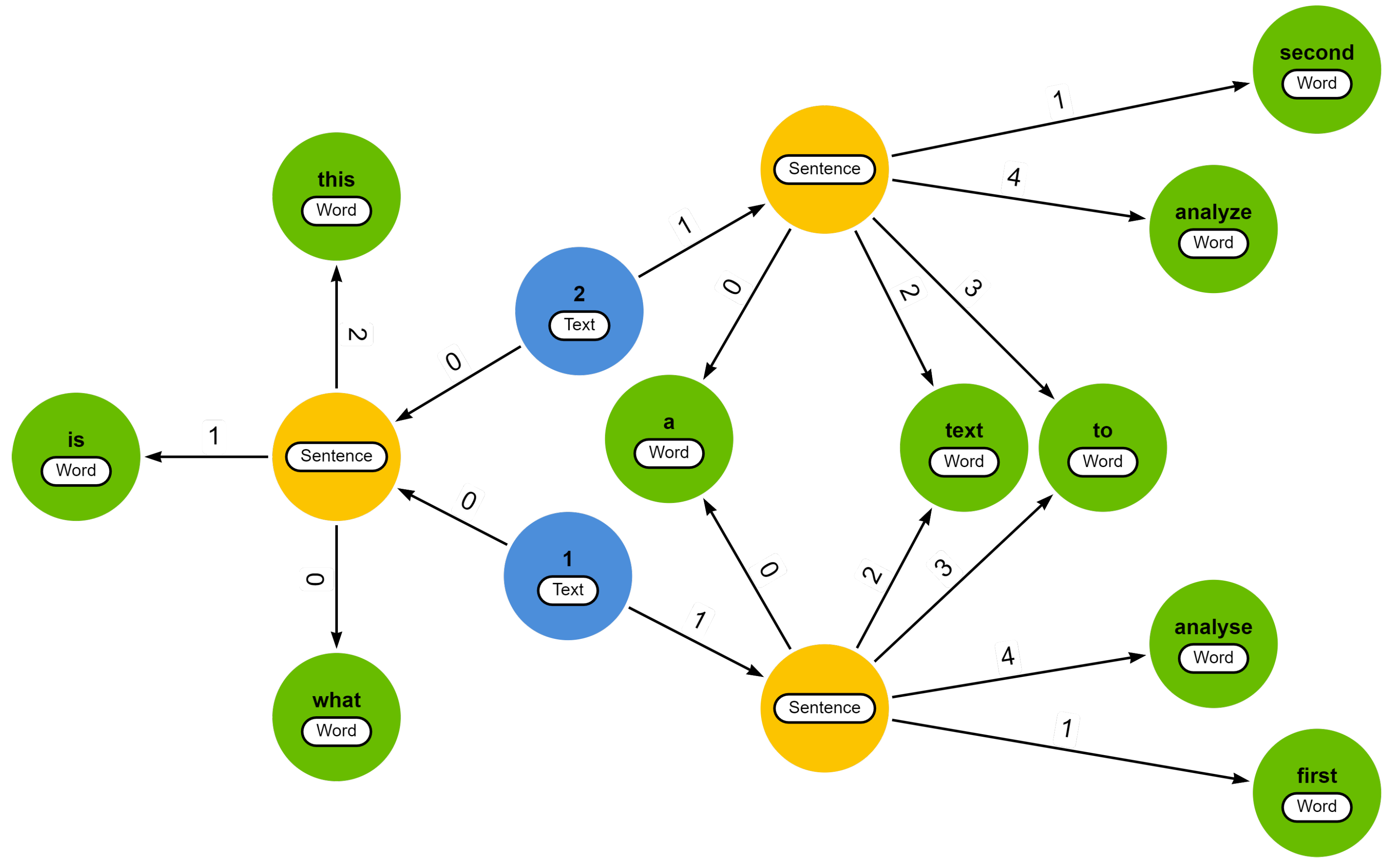
Example 1.

Consider a set of two slightly different texts

T = {“What is this? A first text to analyse.”, “What is this? A second text to analyse.”}

and a list of textual units L = [], where elements with the label  represent a text as a whole. Executing Algorithm 1 on this example results in the graph-based text representation displayed in Figure 1. In this example, the texts are segmented in sentences and, subsequently, the sentences are split into words based on white spaces. Moreover, the texts undergo preprocessing involving the removal of punctuation and the transformation of uppercase letters into lowercase letters.

Algorithm 2 Recursive procedure to construct the different levels of the graph model.

1: procedure ComputeChildNodes($t,i,p$)   2:     $S\leftarrow S\mathrm{P}\mathrm{L}\mathrm{I}\mathrm{T}(t,i)$▹ Text splitting is based on the current discourse unit   3:     for $j\leftarrow 0,\left|S\right|-1$ do   4:         if $\mathrm{a}\mathrm{node}\mathrm{already}\mathrm{exists}\mathrm{on}\mathrm{level}i\mathrm{that}\mathrm{represents}{s}_j$ then   5:            $\mathrm{Define}\mathrm{that}\mathrm{existing}\mathrm{node}\mathrm{as}n$   6:         else   7:            $\mathrm{Create}\mathrm{node}n$   8:            ${\lambda }_N\left(n\right)\leftarrow \left\{l_i\right\}$   9:            if $i>0$ then 10:                ComputeChildNodes$(s_j,i-1,n)$ 11:            else 12:                $\sigma \left(n,\mathsf{text}\right)\leftarrow s_j$ 13:            end if 14:            $N\leftarrow N\cup \left\{n\right\}$ 15:         end if 16:         $\mathrm{Create}\mathrm{edge}e$ 17:         $\rho \left(e\right)\leftarrow \left(p,n\right)$ 18:         $\sigma \left(e,\mathsf{rank}\right)\leftarrow j$ 19:         ${\lambda }_E\left(e\right)\leftarrow \mathtt{CONTAINS}$ 20:         $\tilde{E}\leftarrow \tilde{E}\cup \left\{e\right\}$ 21:         ${\mu }_{\tilde{E}}\left(e\right)\leftarrow 1.0$ 22:     end for 23: end procedure

The first sentence of both texts (left) is represented by a single sentence node, signifying that both (preprocessed) sentences are orthographically identical. The second sentence on the other hand, differs by two words, resulting in a distinct sentence node for each text. In fact, when both texts consist of orthographically identical words, the graph’s structure inherently provides an indication of the similarity between the texts.

Additional text documents can still be included into the graph after its initial construction. This can simply be achieved by re-executing Algorithm 1, with the set T consisting of one or more new text documents, and instead of creating a new graph, the algorithm should use the already constructed graph $\tilde{G}$.

5. A Hierarchical Orthographic Similarity Measure for Graph-Based Text Representations

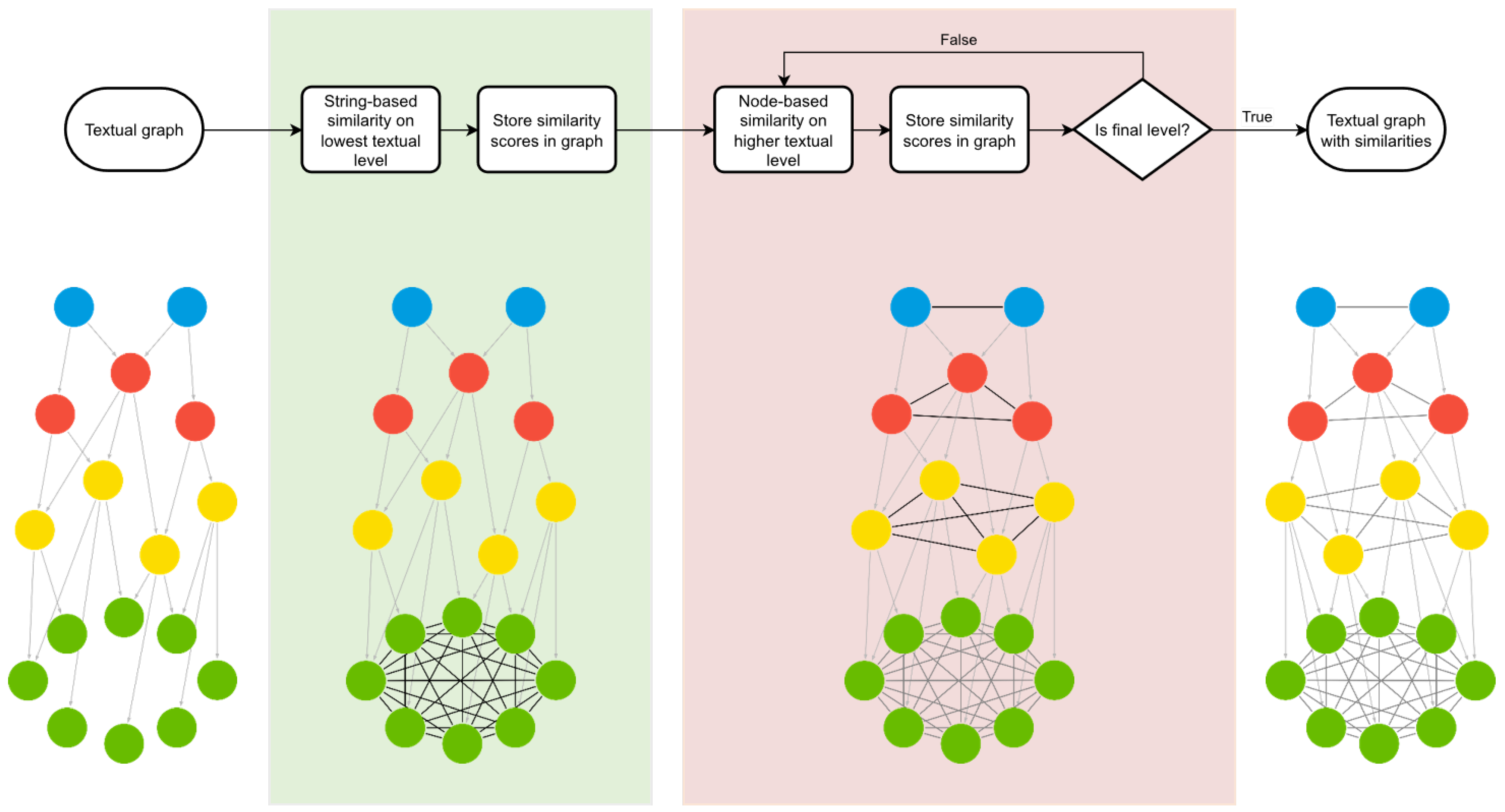
Now that a graph model is in place, representing an entire textual corpus, we propose a novel hierarchical orthographic similarity measure for these graph-based text representations. Analogous to the construction of the textual graph, as proposed in Section 4.2, the hierarchical computation is performed in a bottom-up manner. In Section 5.1, we first propose a string-based similarity measure that computes a pairwise similarity between all nodes representing the smallest textual components in the graph. Next, in Section 5.2, we propose a node-based similarity measure, where a similarity score is hierarchically determined between all nodes situated at the same level. This is achieved by utilising the similarity values between lower-level nodes, calculated in a preceding step. As a result, the graph model for texts is extended with relationships that denote the similarity between all text elements at the same level and between the full texts in the corpus. In Section 5.3, we describe the full computation of our proposed similarity measure and revisit our example from the previous section. A graphical overview of the proposed similarity measure is provided in Figure 2.

5.1. String-Based Similarity Measure

A first step in the hierarchical calculation of the proposed similarity measure consists of calculating the pairwise similarity between all nodes that represent the smallest textual components in the graph. Since these nodes actually contain textual content, a string-based similarity measure is employed. As a similarity measure, we propose a character-based method that is based on the edit distance between two strings.

Calculating this pairwise similarity measure between all lowest-level node pairs, $\left(n_1,n_2\right)\in N_{l_0}^2$ starts by determining the edit distance between the texts contained by those nodes. In this paper, the edit distance is defined as the minimum cumulative cost of edit operations necessary to transform one string into another. The supported edit operations are the insertion, deletion and replacement of a single character, as well as the transposition between two consecutive characters. A formal definition of this string-based edit distance, which is inspired by the Damerau–Levenshtein distance [8], is provided in Definition 4.

Definition 4

(string-based edit distance). Let insertions (I), deletions (D) and replacements (R) of a single character and transpositions (T) between two consecutive characters be the allowed edit operations. The edit distance between two character strings a and b is recursively defined by the function $d_{a,b}^s(i,j)$, whose value is the minimum cost between the prefix of a up to the i-th character and the prefix of b up to the j-th character.

$$d_{a,b}^s\left(i,j\right)=\left\{\begin{array}{cc}\max \left(i,j\right)c_{I,D}\hfill & ,\mathit{if}\min \left(i,j\right)=0\hfill \\ \min \left(\begin{array}{cc}{d}_{a,b}^s(i-1,j)+c_{I,D}\hfill & (I),\\ d_{a,b}^s(i,j-1)+c_{I,D}\hfill & (D),\\ d_{a,b}^s(i-1,j-1)+{\mathbb{1}}_{(a_i\ne b_j)}{c}_R\hfill & (R),\\ d_{a,b}^s(i-2,j-2)+c_T\hfill & (T)\end{array}\right)\hfill & ,\begin{array}{c}\mathit{if}i,j>1\hfill \\ \wedge a_i=b_{j-1}\hfill \\ \wedge a_{i-1}=b_j\hfill \end{array}\hfill \\ \min \left(\begin{array}{cc}{d}_{a,b}^s(i-1,j)+c_{I,D}\hfill & (I),\\ d_{a,b}^s(i,j-1)+c_{I,D}\hfill & (D),\\ d_{a,b}^s(i-1,j-1)+{\mathbb{1}}_{(a_i\ne b_j)}{c}_R\hfill & (R)\end{array}\right)\hfill & ,otherwise\hfill \end{array}\right.$$

(15)

The cost for each edit operation is represented by $c_{*}\in [0,1]$, where ∗ is a placeholder for one of the edit operations $\{(I,D),R,T\}$, and $\mathbb{1}$ is the indicator function.

The cost for the insertion and deletion operations must be equal in order to ensure a symmetric edit distance [47]. When all costs are equal to 1, this edit distance corresponds to the Damerau–Levenshtein edit distance [8]. This proposed string-based edit distance can only be considered a metric when each cost $c_{*}$ is larger than 0. In instances where the cost of any edit operation is 0, the resulting distance between distinct strings can be 0, thereby deviating from the defining properties of a metric [48].

Consider $s_1=\sigma \left(n_1,\mathsf{text}\right)$ and $s_2=\sigma \left(n_2,\mathsf{text}\right)$ as the strings represented by the nodes $n_1$ and $n_2$. The edit distance between those strings is found by the recursive application of Equation (15) and results in a positive real number between 0 and the maximal length (in characters) of both texts (i.e., $\max \left(|s_1|,|s_2|\right)$), depending on the assigned costs for each supported edit operation. As this edit distance indicates dissimilarity rather than similarity between two strings, Equation (16) is required to convert this dissimilarity into a similarity score within the required bounds $\left[0,1\right]$. Note that, since the defined edit distance and the conversion to a similarity are both symmetric, the resulting similarity measure is also symmetric. The calculation of this similarity measure is illustrated in Example 2.

$${\mathrm{sim}}^s(s_1,s_2)=1-\frac{d_{s_1,s_2}^s(|s_1|,|s_2|)}{\max (|s_1|,|s_2|)}$$

(16)

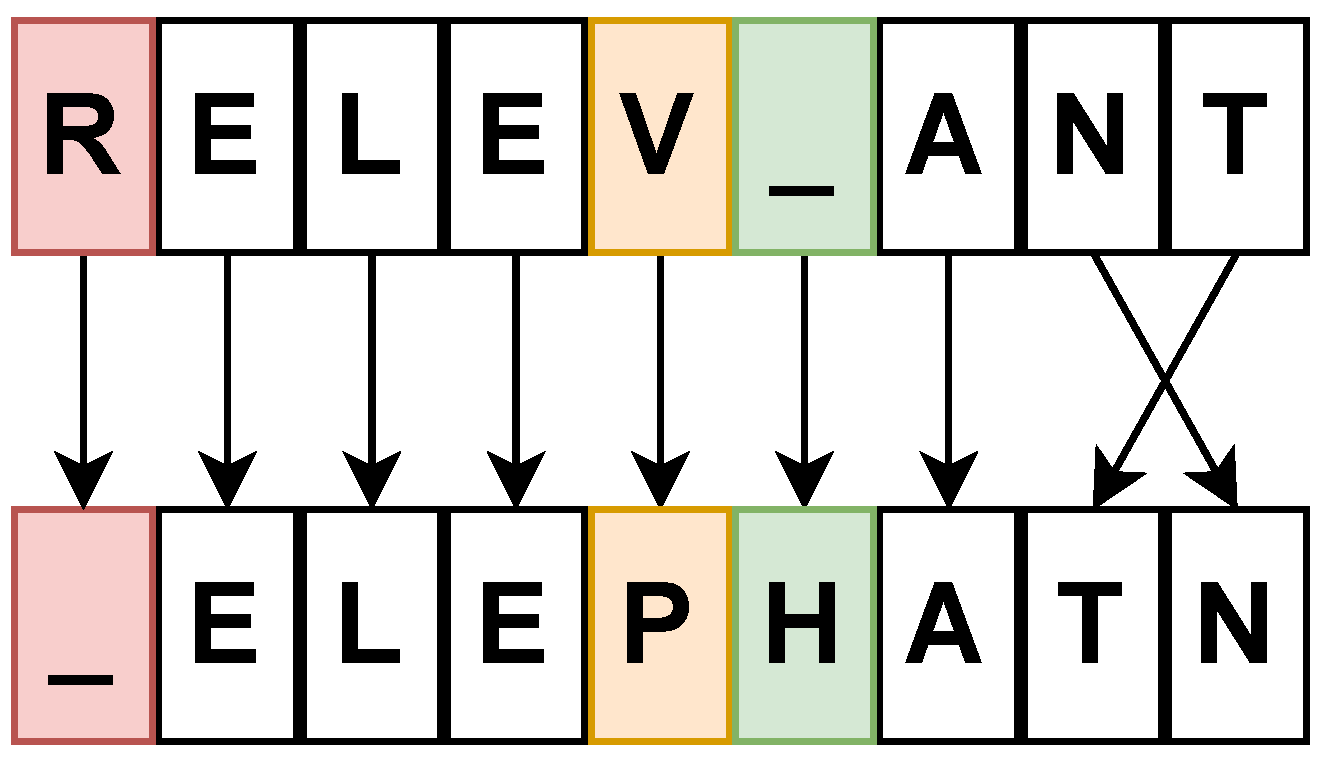
Example 2.

Consider two strings $s_1=\mathtt{RELEVANT}$ and (conveniently misspelled) $s_2=\mathtt{ELEPHATN}$ and all costs $c_{I,D}=c_R=c_T=1$. The minimal edit distance between these two strings can be identified by once performing each of the four supported edit operations, as shown in Figure 3, and is $d_{s_1,s_2}^s(|s_1|,|s_2|)=4$. The similarity score is determined by Equation (16) and is ${\mathrm{sim}}^s(s_1,s_2)=0.5$.

The time complexity of a single edit distance calculation between two strings is $\mathcal{O}\left(\left|s_1\right|·\left|s_2\right|\right)$ and relates to the length of both strings. Since the string-based edit distance is computed on the lowest-level text elements, the strings under consideration are often short and therefore have a manageable execution time. The time complexity of calculating the edit distance on all nodes in $N_{l_0}$, on the other hand, is $\mathcal{O}\left(m^2\right)$, with m equal to the amount of nodes $\left|N_{l_0}\right|$, which can result in performance issues for a very large corpus.

To ascertain the edit distance between two strings, denoted as $s_1$ and $s_2$, a matrix to store all intermediary distances between the prefixes of those strings is required. The dimensions of said matrix are determined by the respective lengths of the aforementioned strings. The implementation can, however, be optimised to store the intermediate results using only two rows, where both rows have the same length as the longest string. As a result, the space complexity of a single edit distance calculation is $\mathcal{O}\left(\max \left(|s_1|,|s_2|\right)\right)$. The space required to store all calculated similarities between all nodes in $N_{l_0}$ is $\mathcal{O}(m^2)$, where m is equal to the amount nodes at that base level of the hierarchy.

Finally, after calculating the similarity scores between all node pairs $(n_1,n_2)$, these similarities are also incorporated into the graph. For that purpose, a new fuzzy edge e is created with label ${\lambda }_E(e)=$ SIMILAR_TO for each obtained similarity score. The membership grade for this new edge is equal to the obtained similarity score

$${\mu }_{\tilde{E}}(e)={\mathrm{sim}}^s(\sigma (n_1,\mathsf{text}),\sigma (n_2,\mathsf{text})).$$

(17)

This new edge is then associated with the related nodes $\rho (e)=(n_1,n_2)$. Since this similarity measure is symmetric, this edge can be interpreted as an undirected edge and is only stored once.

5.2. Node-Based Similarity Measure

As a next step in the calculation of our proposed similarity measure, we calculate the pairwise similarity scores between higher-level text elements in a hierarchical manner. The hierarchical computation follows the order of the hierarchical decomposition, as presented in Section 4.1, starting with all pairs $\left(n_1,n_2\right)\in N_{l_1}^2$. The similarity calculation between all pairs of nodes at the same hierarchical level is repeated for every subsequent level until the similarities between all node pairs $\left(n_1,n_2\right)\in N_{l_n}^2$ representing the entire texts are determined. Just like the string-based similarity measure proposed in the previous section, the node-based similarity measure is based on the edit distance principle. In fact, the node-based similarity measure diverges in only three aspects from the edit distance described in Definition 4.

5.2.1. Child Nodes Instead of Characters

A first difference compared to the edit distance calculation from the previous section is that the node-based edit distance defines its operations on the nodes in a subgraph rather than considering characters in a string. Consider a node $n\in N_{l_i}$, $0<i<\left|L\right|$. The edit distance is calculated on the ordered list of child nodes of n

$$\mathrm{child}(n)=K_n=\left[k_0,k_1,\dots ,k_m\right],$$

(18)

where $k_j\in N_{l_{i-1}}$ and $\rho \left(e_j\right)=\left(n,k_j\right),$ with $e_j\in \mathrm{supp}\left({\tilde{E}}_{\mathtt{CONTAINS}}\right)$ and $j=\sigma \left(e_j,\mathsf{rank}\right)$. Additionally, the number of children $m+1$ of n (i.e., $|\mathrm{child}\left(n\right)|$) is equal to the number of relationships in ${\tilde{E}}_{\mathtt{CONTAINS}}$ between the node n and individual elements of $N_{l_{i-1}}$.

5.2.2. Fuzzy Transposition Matching

Another difference is related to how we determine whether or not a transposition between two consecutive elements actually occurs. In contrast to the string-based edit distance, where a transposition between two consecutive characters is detected in case of an exact match, the node-based edit distance identifies a transposition between two consecutive child nodes by means of a fuzzy match, according to a fixed threshold value $r\in \left[0,1\right]$. Consider two nodes $n_1,n_2\in N_{l_i}$, $0\le i<\left|L\right|$. A fuzzy match between these nodes occurs when

$$\mathrm{match}\left(n_1,n_2\right)={\mu }_{\tilde{E}}\left(e\right)\ge r,$$

(19)

with the edge between both nodes $e\in {\tilde{E}}_{\mathtt{SIMILAR}\_\mathtt{TO}}$ and $\rho \left(e\right)=\left(n_1,n_2\right)$.

5.2.3. Adaptive Replacement Costs

A third and final distinction from the string-based edit distance lies in how the cost of a replacement between child nodes is determined. In the string-based edit distance, a replacement between two characters has a fixed cost $c_R$. The replacement cost in this node-based edit distance is determined by the dissimilarity between a child node and its replacement. This dissimilarity is acquired by subtracting the similarity between two nodes from 1. Additionally, we propose to introduce a similarity threshold $t\in \left[0,1\right]$ as an additional way to deal with orthographic inconsistencies in a corpus. Before calculating the dissimilarity, the similarity between child nodes is assumed to be fully similar (i.e., a similarity score of 1) when the similarity is greater than or equal to the threshold t.

Consider two nodes $n_1,n_2\in N_{l_i},0\le i<\left|L\right|$. The cost of a replacement between these two nodes is determined by the membership function between them

$$c_R\left(n_1,n_2\right)=1-\left(t{\Rightarrow }_{Go}{\mu }_{\tilde{E}}\left(e\right)\right),$$

(20)

where $\rho \left(e\right)=\left(n_1,n_2\right)$ and $e\in {\tilde{E}}_{\mathtt{SIMILAR}\_\mathtt{TO}}$. The similarity threshold t is enforced by means of the Gödel R-implication as defined in Equation (21) [49].

$$p{\Rightarrow }_{Go}q=\left\{\begin{array}{cc}1\hfill & \mathit{if}p\le q\hfill \\ q\hfill & \mathrm{otherwise}\hfill \end{array}\right.$$

(21)

5.2.4. Node-Based Similarity Calculation

Based on the string-based edit distance, described in Section 5.1, and the adaptations described in the previous sections, a full definition for the node-based edit distance is proposed in Definition 5. This edit distance is computed as the minimum cumulative cost of the edit operations required to transform a text element, represented by its child nodes, into another.

Definition 5

(node-based edit distance). Let insertions (I), deletions (D) and replacements (R) of a single node and transpositions (T) between two consecutive nodes be the allowed edit operations. The node-based edit distance between two ordered lists of nodes a and b is recursively defined by the function $d_{a,b}^n\left(i,j\right)$, the value of which is the minimum cost between the prefix of a up to the i-th node and the prefix of b up to the j-th node.

$$d_{a,b}^n(i,j)=\left\{\begin{array}{cc}\max (i,j)c_{I,D}\hfill & ,\mathit{if}\min (i,j)=0\hfill \\ \min \left(\begin{array}{cc}{d}_{a,b}^n(i-1,j)+c_{I,D}\hfill & (I),\\ d_{a,b}^n(i,j-1)+c_{I,D}\hfill & (D),\\ d_{a,b}^n(i-1,j-1)+{\mathbb{1}}_{(a_i\ne b_j)}{c}_R\left(a_i,b_j\right)\hfill & (R),\\ d_{a,b}^n(i-2,j-2)+c_T\hfill & (T)\end{array}\right)\hfill & ,\begin{array}{c}\mathit{if}i,j>1\hfill \\ \wedge \mathrm{match}\left(a_i,b_{j-1}\right)\hfill \\ \wedge \mathrm{match}\left(a_{i-1},b_j\right)\hfill \end{array}\hfill \\ \min \left(\begin{array}{cc}{d}_{a,b}^n(i-1,j)+c_{I,D}\hfill & (I),\\ d_{a,b}^n(i,j-1)+c_{I,D}\hfill & (D),\\ d_{a,b}^n(i-1,j-1)+{\mathbb{1}}_{(a_i\ne b_j)}{c}_R\left(a_i,b_j\right)\hfill & (R)\end{array}\right)\hfill & ,otherwise\hfill \end{array}\right.$$

(22)

The predefined costs for insertions, deletions of single nodes and transpositions of two consecutive nodes are represented by $c_{I,D},c_T\in \left[1,0\right]$. The predefined similarity threshold, utilised to determine the cost of a replacement, and the predefined fuzzy matching threshold, employed to identify transpositions between consecutive nodes, are represented by $t,r\in \left[0,1\right]$, respectively.

Much like the string-based edit distance, this node-based edit distance can only be considered a metric when all edit operation costs are larger than 0. For the replacement cost, this is only the case when the similarity threshold is equal to 1 and when the underlying similarity measure is equal to 0 only when considering the exact same child nodes.

Consider two nodes $n_1,n_2\in N_{l_i},0<i<\left|L\right|$ and their ordered lists of child nodes $K_{n_1}=\mathrm{child}\left(n_1\right)$ and $K_{n_2}=\mathrm{child}\left(n_2\right)$ for which the similarity scores between these child nodes have been predetermined. Just like the string-based edit distance, the node-based edit distance is a measure of dissimilarity and has to be transformed into a similarity measure. This transformation is achieved through the application of the (symmetric) Equation (23).

$${\mathrm{sim}}^n\left(n_1,n_2\right)=1-\frac{d_{K_{n_1},K_{n_2}}^n\left(\left|K_{n_1}\right|,\left|K_{n_2}\right|\right)}{\max \left(\left|K_{n_1}\right|,\left|K_{n_2}\right|\right)}$$

(23)

We can now show the following properties of this node-based similarity measure.

Proposition 1.

The node-based similarity in Equation (23) is reflexive:

$${\mathrm{sim}}^n\left(n_1,n_1\right)=1,\forall n_1\in N_i,\forall 0<i<\left|L\right|$$

Proof. 

Consider $K_{n_1}=\mathrm{child}(n_1)$ as the ordered sequence of children of the node $n_1$. The node-based edit distance in Equation (22) results in $d_{K_{n_1},K_{n_1}}^n\left(\left|K_{n_1}\right|,\left|K_{n_1}\right|\right)=0$ since no transformations are required to transform $K_{n_1}$ into itself. It follows that Equation (23) results in a similarity score of 1.    □

Proposition 2.

The node-based similarity in Equation (23) is symmetric:

$${\mathrm{sim}}^n\left(n_1,n_2\right)={\mathrm{sim}}^n\left(n_2,n_1\right),\forall n_1,n_2\in N_i,\forall 0<i<\left|L\right|$$

Proof. 

Proof by induction on i, the level in the hierarchy.

• Base step: If $i=0$, similarity is computed with the string-based similarity (Equation (16)), where the underlying string-based edit distance is symmetric by definition [47]. Since the max operator is also symmetric, it follows that the string-based similarity is symmetric, which settles the base case.
• Inductive step: Assume that the similarity measure at level $i\ge 0$ is symmetric, we prove that the node-based similarity at level $i+1$ is also symmetric. Since it is clear that the max operator is symmetric, this suffices to prove that the underlying node-based edit distance used in Equation (23) is symmetric. An edit distance is symmetric when it has a reverse operation for every edit operation with the same cost [47]. Insertions and deletions are reverse operations of each other and have the same fixed cost as stated in Definition 5. Replacements, on the other hand, are their own reverse operations. The cost of replacements, as shown by Equation (20), depends on the similarity scores between nodes at level i. Since the similarity measure at level i is symmetric, it follows that the costs of reversed replacement operations for the same child nodes are equal to each other. Finally, transpositions always have a fixed cost and are the reverse operations of themselves if their fuzzy match operator is symmetric. Because this operator, as stated in Equation (19), is fully determined by the similarity scores at level i, it is also symmetric. By showing that the four edit operations always have a reversed operation with the same cost, it follows that the node-based edit distance and consequently the node-based similarity are symmetric.

   □

The calculation of the proposed node-based similarity measure is now illustrated in Example 3.

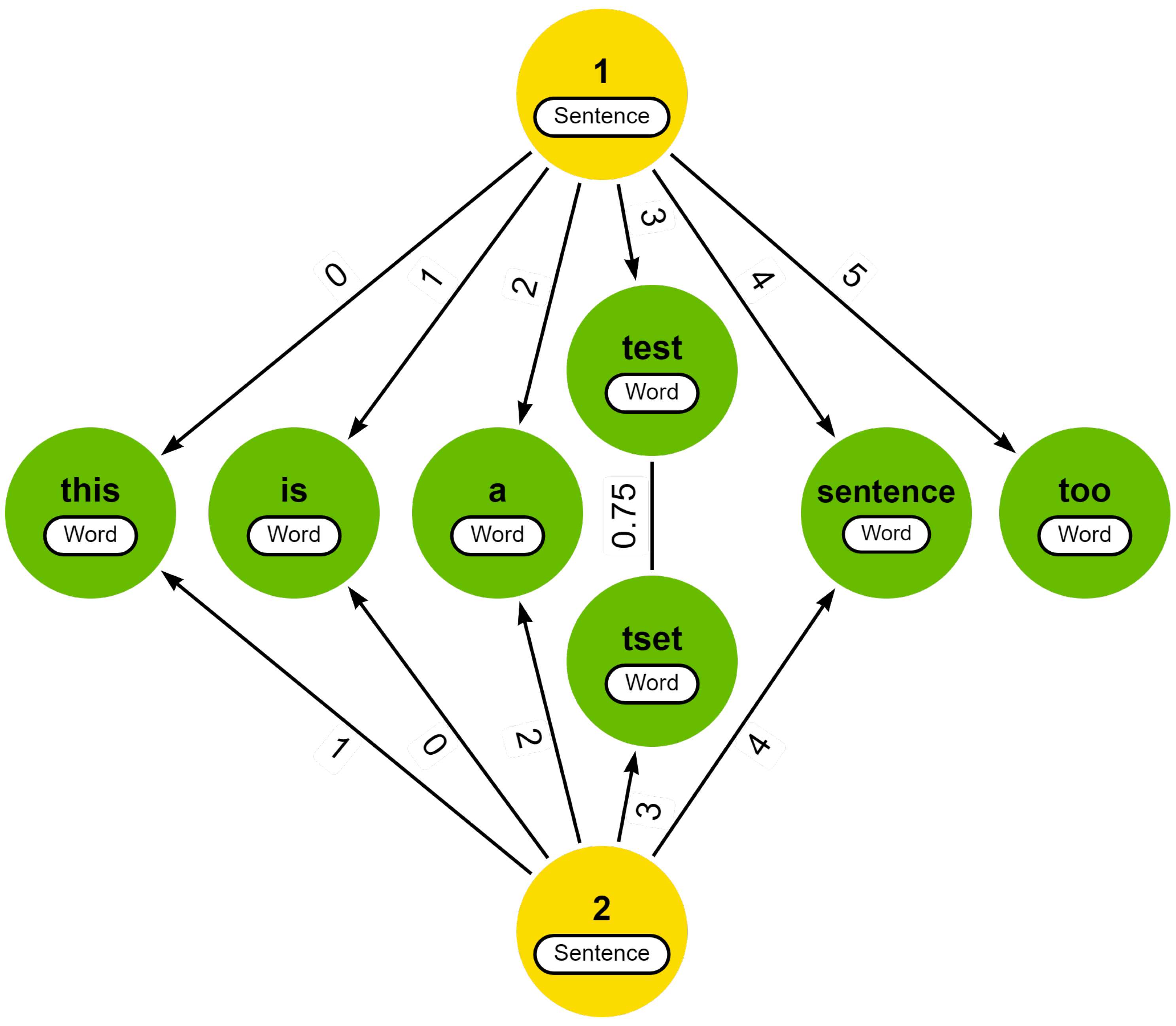
Example 3.

Consider a set of two slightly different texts

T = {“This is a test sentence too.”, “Is this a tset sentence?”},

with a hierarchical decomposition into L = [] and a typo for the word “test” in the second text. The graph-based text representation for this small corpus is displayed in Figure 4. The relevant similarity scores between words have already been determined. In this example, we assume that the costs for the edit operations, the similarity threshold and the fuzzy match threshold for the node-based edit distance are all set equal to 1.

To calculate the similarity, it is necessary to first determine the edit distance between the child nodes. Based on the edit operation costs, the minimum edit distance for this example is found by (i) a transposition between the first two nodes, with a cost of 1, (ii) a replacement of the word “test” with the word “tset”, with a cost equal to the dissimilarity between those words (i.e., $0.25$), and (iii) an insertion (or deletion) of the last node, with a cost of 1. As a result, the edit distance equals $2.25$, and the similarity, as per Equation (23), equals $0.625$.

Now imagine another scenario where the similarity threshold t is $0.75$ leading to a replacement cost of 0 between the words “test” and “tset”. Therefore, the similarity score between the two sentences results in $0.666\dots$.

The time complexity of a single node-based edit distance calculation between node $n_1$ and $n_2$ is related to the length of both lists of child nodes and is equal to $\mathcal{O}\left(\left|\mathrm{child}(n_1)\right|·\left|\mathrm{child}(n_2)\right|\right)$. Since the amount of child nodes at any level of the hierarchy depends on the hierarchical decomposition of the considered texts, the execution time can be kept within reasonable bounds by adopting a hierarchical decomposition that results in a short list of child nodes. Additionally, much like the string-based similarity measure, the time complexity of calculating the similarities on all nodes in $N_{l_i}$, with $0<i<\left|L\right|$ and m equal to the amount of nodes in $N_{l_i}$, is $\mathcal{O}(m^2)$.

The space requirements of the node-based edit distance are equal to the space complexities of the string-based edit distance, as described in Section 5.1, except for the space complexity of a single node-based edit distance calculation, which now relates to the length of two child node lists instead of to the length of two strings.

5.3. Graph-Based Text Model with Similarities

With the various components of our similarity measure in place, we can now describe our proposed hierarchical orthographic similarity measure in full. The procedure for the computation of the similarity values between all text elements, and most importantly between all full texts, is provided in Algorithm 3.

Algorithm 3 Similarity calculation in the graph-based text representation.

Input: $\mathrm{A}\mathrm{fuzzy}\mathrm{graph}\tilde{G}\left(N,\tilde{E},\rho ,{\lambda }_N,{\lambda }_E,\sigma \right)\mathrm{representing}\mathrm{the}\mathrm{texts}\mathrm{in}\mathrm{a}\mathrm{corpus}$ Output: $\mathrm{The}\mathrm{fuzzy}\mathrm{graph}\tilde{G}\mathrm{with}\mathrm{the}\mathrm{calculated}\mathrm{similarity}\mathrm{scores}$   1: for $i\leftarrow 0,\left|L\right|-1$ do   2:     $\mathrm{Determine}\mathrm{parameters}{c}_{I,D},c_R\mathrm{and}{c}_T\mathrm{or}{c}_{I,D},c_T,r\mathrm{and}t$   3:     for all $\left(n_1,n_2\right)\in N_{l_i}^2$ do   4:         if $i=0$ then   5:            $s=si{m}^s\left(\sigma \left(n_1,\mathsf{text}\right),\sigma \left(n_2,\mathsf{text}\right)\right)$   6:         else   7:            $s=si{m}^n\left(n_1,n_2\right)$   8:         end if   9:         $\mathrm{Create}\mathrm{edge}\mathrm{e}$ 10:         $\rho \left(e\right)\leftarrow \left(n_1,n_2\right)$ 11:         ${\lambda }_E\left(e\right)\leftarrow \mathtt{SIMILAR}\_\mathtt{TO}$ 12:         $\tilde{E}\leftarrow \tilde{E}\cup \left\{e\right\}$ 13:         ${\mu }_{\tilde{E}}\left(e\right)\leftarrow s$ 14:     end for 15: end for 16: $\mathbf{return}\tilde{G}\left(N,\tilde{E},\rho ,{\lambda }_N,{\lambda }_E,\sigma \right)$

In this algorithm, we hierarchically compute the pairwise similarity for all node pairs sharing a specific label. For the lowest-level text elements, the string-based similarity proposed in Section 5.1 is used. The similarities between all other text elements sharing the same label are determined by the node-based similarity, as described in Section 5.2. Note that the parameters $c_{I,D},c_R$ and $c_T$ for the string-based similarity and parameters $c_{I,D},c_T,r$ and t for the node-based similarity may vary at each level within the hierarchy but remain fixed throughout the calculations within a specific level. As a result, each parameter at every level of the hierarchical calculation can be fine-tuned, either through expert knowledge or empirical analysis, to suit the specifics of a given corpus. Once the similarity between two nodes is determined, a new edge is created to indicate the similarity between those two elements. As the similarity measure between two nodes is symmetric, only a single undirected edge is created between the nodes. Upon completion of the procedure, the graph-based text representation is returned, including the similarity scores between all elements within the same discourse unit. As an illustration, the result of the hierarchical computation between two texts is provided in Example 4.

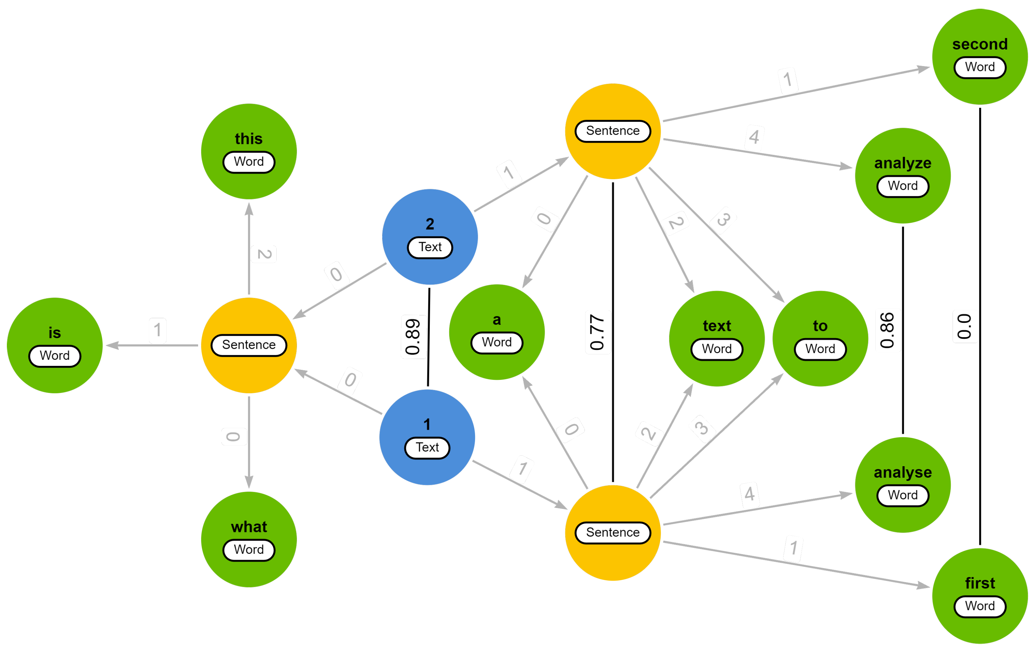
Example 4.

In Figure 5, we revisit our textual graph from Example 1 and display the similarity scores between all text elements that are required to compute the similarity between both full texts. For the calculation of this example, all parameters $c_{I,D},c_R,c_T,t$ and r are equal to 1 for every level.

The time required to calculate the the similarities between all nodes on every level of the graph is equal to the sum of the calculation time at every level of the hierarchy. In Section 5.1 and Section 5.2, we concluded that the time required for every level is $\mathcal{O}(n_i)$, where $n_i$ is equal to the amount of nodes at a specific level $\left|N_{l_i}\right|$ and $0\le i<\left|L\right|$. Since the time complexity is dominated by the largest term, the overall time complexity is equal to $\mathcal{O}\left({\max }_i{n}_i^2\right)$.

The space complexity of the complete algorithm, on the other hand, is equal to the largest space requirement among the different hierarchical levels. As a result, the space complexity is also equal to $\mathcal{O}\left({\max }_i{n}_i^2\right)$.

After the initial computation of the similarity values between text elements in the graph, there remains the possibility of incorporating additional text documents into this graph. First, the new texts should be included into the graph as described in Section 4.2. Then, only the additional similarity values between the newly added nodes and all existing nodes at the same hierarchical level should be computed in the same manner as outlined in Algorithm 3.

6. Experiments

In this section, we demonstrate and motivate the relevance of the proposed technique by its use as a research tool for the analysis of ancient texts and compare it to another state-of-the-art soft measure. In Section 6.1, we illustrate the characteristics of Byzantine book epigrams [50], the corpus used as a dataset in the following experiments. Then, we discuss the graph-based text representation of this corpus and the methods used in the experiments in Section 6.2. In Section 6.3, we describe the setup of the experiments alongside the methods employed for evaluating the proposed similarity measure. Next, we list and discus the results of our experiments in Section 6.4. Lastly, in Section 6.5, we provide an illustrative example, where we show the interactive capabilities of the proposed graph model implemented in a graph database.

6.1. Dataset: Byzantine Book Epigrams

Byzantine book epigrams are poems nestled in the margins of medieval Greek manuscripts. They are typically short and tell the reader more about, for instance, the manuscript’s content, the individuals involved in its production or even the emotions experienced by the scribe upon completing the manuscript. These epigrams are typically known to be orthographically inconsistent texts with a complex tradition. That is a tradition, or in other words the transmission of the texts throughout history, in which texts were split-up, (re)combined or elseways reworked during their copying process. As a result of this complex tradition, where combinations of words and (half)verses are often re-used throughout a variety of epigrams, the corpus of Byzantine book epigrams displays an expansive amount of interconnections among its texts [41,50].

The orthographic irregularities displayed in these book epigrams arise not solely from factors like spelling and transcription errors, unstandardised punctuation, and text wrapping. They are also caused by the evolution of the Greek language. Particularly noteworthy is the phonetic evolution known as itacism. Itacism denotes the shift of the classical pronunciation of the vowels ι, η, υ, ῃ and the diphthongs ει, οι converging towards the pronunciation of i. This results in a corpus where all the aforementioned vowels and diphthongs are used interchangeably [41,50,51]. The complex and interconnected nature of these Byzantine book epigrams makes them an ideal corpus for evaluating the capabilities of the proposed similarity measure.

The Database of Byzantine Book Epigrams (DBBE) (https://dbbe.ugent.be, accessed on 1 February 2024) [50,52] is composed of experts and contains an extensive collection of Byzantine book epigrams, complemented by manually composed groups of similar texts. These groups of similar texts within the DBBE serve as a ground truth for evaluating the proposed similarity measure. Two categories of such groups exist in the DBBE: those comprising similar epigrams and those composing similar verses. Since these groups are manually composed by experts, they include texts that are only partially known or variants of a text where synonyms are used.

For the experiments, a representative subset for each category of these groups is carefully identified by experts and exported from the DBBE dataset. The subset of verses is composed of the verses contained in the verse groups with identifiers 15681, 15470, 14667, 11233, 14852, 12251, 15904, 14932, 14802, 10671, 4634, 15377, 12290, 14866, 15278, 12121, 13035, 15327, 6342, 5549, 445, 2520, 3949, 5354, 5840, 6353, 9033, 10869, 12122, 15261, 15652 and 14872, resulting in a subset of 750 verses to be compared. Additionally, the subset of epigrams is composed of the epigram groups with identifiers 2148, 2150, 4245, 2326, 3147, 3436, 4152, 4155, 5030, 5248, 6473, 1953, 6475, 1862, 1982, 2225, 3987, 2311, 31190, 3762, and 2054, resulting in a subset consisting of 500 epigrams.

Because of the complex orthographic characteristics of Byzantine book epigrams, the original epigrams and verses from the selected datasets need to undergo preprocessing before we use them in our experiments in order to standardise the texts and reduce noise. First, all uppercase letters are converted to their lowercase counterparts. The next step involves the removal of any punctuation or other special characters. All accents and other diacritical marks are then stripped off, because of the frequent occurrence of unstandardised accentuation in these epigrams [41,50]. In the fourth and final step, all vowels η, υ, ῃ and the diphthongs ει, οι are systematically replaced with ι in order to tackle with the phenomenon of itacism.

6.2. Methods

In the experiments, two methods for text similarity are considered. The first method is the similarity measure proposed in this paper, with different values for various parameters. Before the similarity scores can be determined, the corpus must be transformed into a graph-based representation. The transformation of a set T, representing a corpus of Byzantine book epigrams, into the required graph representation is accomplished through Algorithm 1. To successfully execute this algorithm, certain design decisions, related to the given corpus, must first be made.

As discussed in the previous section, words, half verses and verses are the key textual elements contributing to the interconnected nature of Byzantine book epigrams. Given that half verses are not stored in the DBBE and no (well-performing) automatic method for their identification exists, the discourse units that make up the hierarchical decomposition of epigrams, and therefore define the structure of the graph, are $L=\left[\mathtt{Word},\mathtt{Verse},\mathtt{Epigram}\right]$.

As a last step in defining the graph representation, the procedures for segmenting the text documents into smaller components need to be determined. Given that the DBBE stores epigrams as a list of verses, extracting the verses directly from the database is a straightforward process. Conversely, the identification of words is accomplished by partitioning the verses based on white spaces.

Based on this graph representation, we have implemented our approach using two Neo4j (https://www.neo4j.org, accessed on 1 February 2024) databases: one for the subset of verses and one for the subset of epigrams. The proposed hierarchical similarity measure for Byzantine book epigrams is implemented as a Neo4j plugin (the Java code for this Neo4j plugin can be found at https://github.com/MaximeDeforche/DBBESimilarity, accessed on 1 February 2024) and can be executed on the graph (database) by providing it with valid cost and threshold values for every level of the hierarchical decomposition.

The second method we include in the experiments is a state-of-the-art soft similarity measure that combines the idea of token-based and character-based similarity [15,16]. More specifically, this method computes the similarity between two texts by first transforming each text into a bag of tokens. Then, each token from the first bag is compared with each token from the second bag by means of a token matcher. The result of this comparison is a similarity score for both tokens. All token similarities are stored in a matrix that is used to compute a leximax-optimal assignment between tokens from both bags. Based on this assignment, a sequence of scores is obtained, and this sequence is aggregated into a final score by using a weighted minimum. The weights are computed by means of a parameterised quantifier function. Because of this two-step methodology, where one first computes similarities on the level of tokens and then on the level of bags, the method is called a two-level string matcher.

The two-level string matcher has some properties that are relevant to mention in the context of the experiments we report. First, by using a bag model, it neglects the order of tokens in a text completely. Second, the token matcher can account for spelling errors on the level of tokens, for example, by using edit distances to compare tokens. The original method, however, uses a dedicated token matcher that is designed to be fast and to produce similarity matrices that are sparse. Third, if two bags of tokens have different cardinalities, a quantifier function allows us to model the influence of the difference in cardinality on the final similarity. The choice of this function can influence the effectiveness of the two-level matcher significantly [16], and it therefore needs to be chosen with care. An implementation of the two-level string matcher is available in Java as part of the ledc-framework (https://ledc.ugent.be/, accessed on 1 February 2024) and can be found on GitLab (https://gitlab.com/ledc/ledc-match, accessed on 1 February 2024).

6.3. Experiment Setup

In the first experiment, we want to assess the capabilities and usefulness of our proposed method. For each of the two Neo4j databases, we have conducted three distinct similarity calculations, each with different parameter settings. The three sets of parameter values are listed in

Table 1. Different sets of parameter values for the first experiment.

Level	Parameter	Default	Custom 1	Custom 2
	$c_{I,D}$	$1.0$	$0.9$	$0.8$
Word	$c_T$	$1.0$	$0.9$	$0.0$
	$c_R$	$1.0$	$1.0$	$1.0$
Verse	$c_{I,D}$	$1.0$	$0.9$	$0.8$
	$c_T$	$1.0$	$0.0$	$0.0$
	t	$1.0$	$0.9$	$0.8$
	r	$1.0$	$0.8$	$0.7$
Epigram	$c_{I,D}$	$1.0$	$0.95$	$0.85$
	$c_T$	$1.0$	$0.0$	$0.0$
	t	$1.0$	$0.9$	$0.8$
	r	$1.0$	$0.8$	$0.7$

, where the parameters used for the Word level relate to the parameters of the string-based edit distance in Equation (15). The parameters used for the Verse and Epigram levels, on the other hand, relate to the parameters of the node-based edit distance in Equation (22). The first parameter set resembles the default values for all parameters, whereas the other two parameter sets reduce the cost for edit operations, as well as lower the thresholds for similarity and transposition matching. These adjustments increase the tolerance for certain (minor) differences between texts as a way to optimise the similarity measure for the given corpus.

In the second experiment, we compute similarities on both datasets with the two-level string matcher. We did so with two different token matchers. The first token matcher is the default token matcher for the two-level string matcher [15]. Using this default matcher yields sparse similarity matrices, resulting in faster resolution of assignments. In the current experiment, however, this might also lead to many pairs of tokens that are wrongly assigned a similarity of zero. To deal with this, we also use a token matcher that is based on the Damerau distance. This second token matcher is the same as the one that we used on the Word-level in our approach, with the exception that distances above 3 resulted in a similarity of 0. The latter was necessary to ensure that the two-level string matcher finished within a reasonable time.

Next to the token matcher, we must also choose a quantifier function for weight computation. We found empirically that the default parameters of this function are too strict in the scope of the current experiment, and that better results were obtained when setting the main quantifier parameter $\alpha$ to $0.9$.

The results of both experiments can be expressed by means of a fuzzy similarity relation $\tilde{S}$, representing the pairwise similarity between two epigrams or verses. In order to compare the resulting similarities in both experiments against the crisp definition of similar texts in the ground truth, which are assigned by experts, we perform an $\alpha$-cut on the resulting fuzzy similarity relation $\tilde{S}$. For each remaining pair of verses or epigrams in the relation (after the $\alpha$-cut), it is checked whether the verse or epigram pair is also similar according to the ground truth. If this is the case, it leads to a true positive (TP), and when it is not the case, it results in a false positive (FP). Likewise, all pairs of verses and epigrams that were pruned by the $\alpha$-cut are checked in the same manner. Pruned pairs linking two verses or epigrams that are similar according to the ground truth are counted as false negatives (FN), whereas the others are counted as true negatives (TN). These four values enable the calculation of various quality measures offering insight into the performance of the different similarity measures concerning individual verses or full epigrams, according to the provided parameter values and a given $\alpha$ value.

As a first quality measure, we calculate the recall of the proposed similarity measure

$$\mathrm{recall}=\frac{\mathrm{TP}}{\mathrm{TP}+\mathrm{FN}},$$

(24)

where the fraction of successfully identified similar texts is determined. Secondly, we calculate the precision:

$$\mathrm{precision}=\frac{\mathrm{TP}}{\mathrm{TP}+\mathrm{FP}}.$$

(25)

The precision depicts the fraction of correctly identified similar texts among all identified similar texts. As a third and last quality measure, we compute the F₁-score. This is the harmonic mean of the precision and recall:

$${\mathrm{F}}_1-\mathrm{score}=2·\frac{\mathrm{precision}·\mathrm{recall}}{\mathrm{precision}+\mathrm{recall}}.$$

(26)

The F₁-score provides us with a single value that indicates an overall performance of the similarity measure, balancing precision and recall into a single measure.

For each similarity calculation in both experiments, we have calculated these quality measures for a set of nine distinct $\alpha$ values, ranging from $0.1$ till $0.9$. Ultimately, the quality measures are computed for 54 different situations in the first experiment and for 36 situations in the second experiment.

6.4. Results

Table 2. Summary of experimental results of the first experiment using the proposed similarity measure. The employed parameter sets are listed in Table 1. The highest scores for each column are indicated in bold.

Similarity Parameters	Threshold $\mathit{\alpha }$	Verses			Epigrams
		Precision	Recall	F1-Score	Precision	Recall	F1-Score
	$0.1$	$0.1627$	$0.9984$	$0.2797$	$0.1638$	$0.9904$	$0.2811$
	$0.2$	$0.4305$	$0.9932$	$0.6007$	$0.5387$	$0.9741$	$0.6937$
	$0.3$	$0.8831$	$0.9831$	$0.9304$	$0.5741$	$0.9499$	$0.7156$
	$0.4$	$0.9609$	$0.9715$	$0.9661$	$0.6049$	$0.9147$	$0.7283$
Default	$0.5$	$0.9782$	$0.9417$	$0.9596$	$0.6687$	$0.8589$	$0.7520$
	$0.6$	$0.9986$	$0.8688$	$0.9292$	$0.7745$	$0.7757$	$0.7751$
	$0.7$	$\mathbf{1}.\mathbf{0000}$	$0.7452$	$0.8540$	$0.8559$	$0.6796$	$0.7576$
	$0.8$	$\mathbf{1}.\mathbf{0000}$	$0.6059$	$0.7546$	$0.8786$	$0.5599$	$0.6840$
	$0.9$	$\mathbf{1}.\mathbf{0000}$	$0.3398$	$0.5072$	$0.9365$	$0.3778$	$0.5384$
	$0.1$	$0.1455$	$\mathbf{1}.\mathbf{0000}$	$0.2540$	$0.0889$	$0.9998$	$0.1632$
	$0.2$	$0.2112$	$0.9951$	$0.3485$	$0.3515$	$0.9829$	$0.5178$
	$0.3$	$0.6899$	$0.9910$	$0.8135$	$0.5636$	$0.9574$	$0.7095$
	$0.4$	$0.9518$	$0.9833$	$0.9673$	$0.5992$	$0.9318$	$0.7294$
Custom 1	$0.5$	$0.9718$	$0.9621$	$0.9669$	$0.6492$	$0.8923$	$0.7518$
	$0.6$	$0.9978$	$0.8980$	$0.9453$	$0.7424$	$0.8123$	$0.7758$
	$0.7$	$0.9999$	$0.7885$	$0.8817$	$0.8759$	$0.7187$	$\mathbf{0}.\mathbf{7896}$
	$0.8$	$\mathbf{1}.\mathbf{0000}$	$0.6442$	$0.7836$	$0.8895$	$0.5977$	$0.7150$
	$0.9$	$\mathbf{1}.\mathbf{0000}$	$0.3643$	$0.5340$	$\mathbf{0}.\mathbf{9731}$	$0.4354$	$0.6016$
	$0.1$	$0.1447$	$\mathbf{1}.\mathbf{0000}$	$0.2529$	$0.0798$	$\mathbf{1}.\mathbf{0000}$	$0.1478$
	$0.2$	$0.1502$	$\mathbf{1}.\mathbf{0000}$	$0.2611$	$0.0998$	$0.9998$	$0.1815$
	$0.3$	$0.3028$	$0.9948$	$0.4642$	$0.5155$	$0.9800$	$0.6756$
	$0.4$	$0.8616$	$0.9895$	$0.9211$	$0.5727$	$0.9562$	$0.7163$
Custom 2	$0.5$	$0.9633$	$0.9777$	$\mathbf{0}.\mathbf{9704}$	$0.6041$	$0.9236$	$0.7305$
	$0.6$	$0.9854$	$0.9343$	$0.9592$	$0.6555$	$0.8634$	$0.7452$
	$0.7$	$0.9995$	$0.8576$	$0.9231$	$0.7255$	$0.7954$	$0.7588$
	$0.8$	$\mathbf{1}.\mathbf{0000}$	$0.7065$	$0.8280$	$0.8834$	$0.6882$	$0.7737$
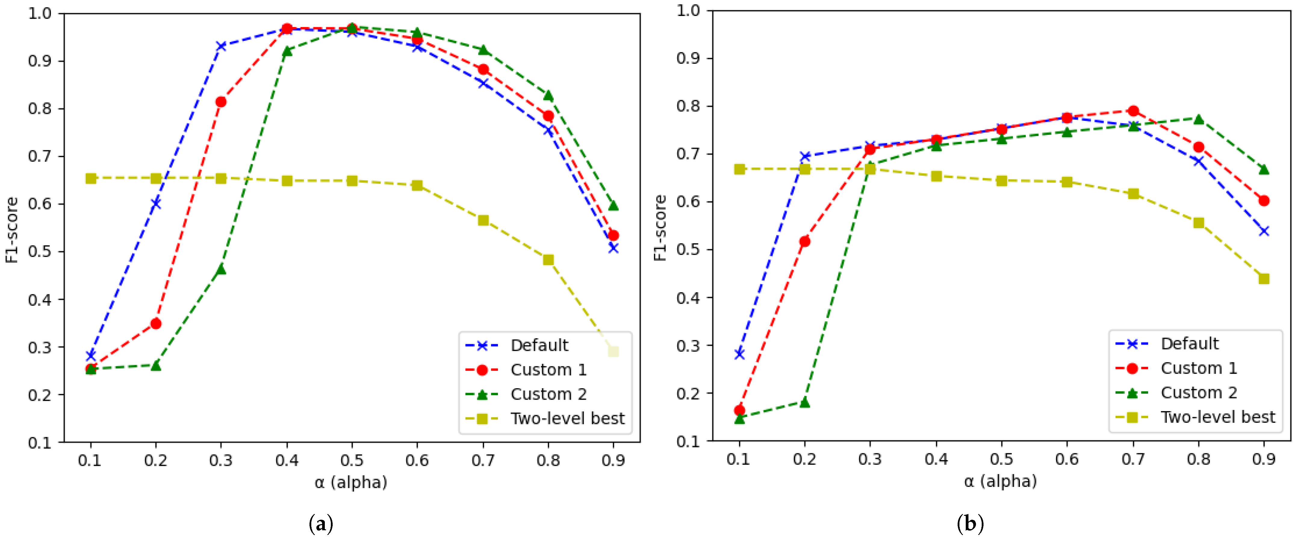
	$0.9$	$\mathbf{1}.\mathbf{0000}$	$0.4253$	$0.5968$	$0.8873$	$0.5352$	$0.6677$

showcases the results of the calculated quality measures for the verse and epigram test sets and three distinct parameter sets in our first experiment. In each column, the highest value for each performance measure is highlighted in bold. Additionally, the F₁-score results for verses and epigrams are visualised by plots in Figure 6a and Figure 6b, respectively.

In the case of verses, we observe the same trend across all three parameter sets. For low $\alpha$ values, we find a very high recall but a very low precision. This suggests that (nearly) all similar texts are detected, albeit at the expense of misclassifying numerous text pairs as similar. With high $\alpha$ values, we observe the reverse scenario, coupled with a slightly higher F₁-score. The peak overall performance for verses is achieved with the third, most tolerant parameter set (i.e., the second custom parameter set) and an $\alpha$ threshold of $0.5$.

For epigrams, the resulting values are generally lower in comparison to verses, yet the same trend can be observed across the three parameter sets. The lower scores are explained by the fact that these epigrams can structurally vary in more ways than the individual verses, coupled with the increased potential for orthographic inconsistencies in longer texts. Overall, the best score for the epigram test set is achieved by using the second set of parameters with an $\alpha$ value of $0.7$.

In general, the choice of the hierarchical decomposition of a text and the parameters choices for each level in the hierarchical computation of the similarity can significantly influence the performance of the similarity measure. The high customisability of the proposed method provides the flexibility to fine-tune numerous parameters when determining the optimal parameter set for a given corpus. This adaptability also empowers researchers to carefully select each parameter based on the specific requirements of a textual analysis. Furthermore, the possibility to chose an $\alpha$ value allows us to indicate whether we want to identify more similar texts (higher recall), be more certain about the identified text pairs (higher precision) or strike a balance between the two. Lastly, it is noteworthy that using more tolerant parameter sets can, up to some point, enhance the overall performance of the similarity measure and the similarity scores between genuinely similar texts. However, making the parameter sets too tolerant for structural and orthographic variations between texts results in a suboptimal performance of the proposed measure.

Considering the fact that not all possible orthographic inconsistencies can be automatically dealt with and that the expert-based similarity groups, which serve as the ground truth, include texts that are only partially complete and/or contain variations where synonyms are used, the proposed orthographic similarity measure shows encouraging results.

Table 3. Summary of experimental results of the second experiment using a two-level string matcher. The highest scores for each column are indicated in bold.

Similarity Parameters	Threshold $\mathit{\alpha }$	Verses			Epigrams
		Precision	Recall	F1-Score	Precision	Recall	F1-Score
	$0.1$	$0.9992$	$\mathbf{0}.\mathbf{4860}$	$\mathbf{0}.\mathbf{6539}$	$0.6798$	$\mathbf{0}.\mathbf{6559}$	$\mathbf{0}.\mathbf{6676}$
	$0.2$	$0.9992$	$\mathbf{0}.\mathbf{4860}$	$\mathbf{0}.\mathbf{6539}$	$0.6797$	$0.6557$	$0.6675$
	$0.3$	$0.9992$	$\mathbf{0}.\mathbf{4860}$	$\mathbf{0}.\mathbf{6539}$	$0.6797$	$0.6556$	$0.6674$
	$0.4$	$0.9999$	$0.4788$	$0.6476$	$0.6783$	$0.6294$	$0.6529$
Two-Level (Damerau)	$0.5$	$0.9999$	$0.4788$	$0.6476$	$0.6739$	$0.6158$	$0.6435$
	$0.6$	$\mathbf{1}.\mathbf{0000}$	$0.4688$	$0.6383$	$0.6799$	$0.6062$	$0.6409$
	$0.7$	$\mathbf{1}.\mathbf{0000}$	$0.3952$	$0.5665$	$0.7097$	$0.5438$	$0.6158$
	$0.8$	$\mathbf{1}.\mathbf{0000}$	$0.3192$	$0.4840$	$0.7208$	$0.4536$	$0.5568$
	$0.9$	$\mathbf{1}.\mathbf{0000}$	$0.1694$	$0.2898$	$\mathbf{0}.\mathbf{8115}$	$0.3019$	$0.4401$
	$0.1$	$\mathbf{1}.\mathbf{0000}$	$0.2738$	$0.4299$	$0.7383$	$0.4236$	$0.5383$
	$0.2$	$\mathbf{1}.\mathbf{0000}$	$0.2734$	$0.4294$	$0.7394$	$0.4210$	$0.5365$
	$0.3$	$\mathbf{1}.\mathbf{0000}$	$0.2733$	$0.4293$	$0.7391$	$0.4193$	$0.5351$
	$0.4$	$\mathbf{1}.\mathbf{0000}$	$0.2729$	$0.4288$	$0.7372$	$0.4154$	$0.5313$
Two-Level (Default)	$0.5$	$\mathbf{1}.\mathbf{0000}$	$0.2728$	$0.4287$	$0.7328$	$0.4051$	$0.5218$
	$0.6$	$\mathbf{1}.\mathbf{0000}$	$0.2724$	$0.4281$	$0.7316$	$0.4025$	$0.5193$
	$0.7$	$\mathbf{1}.\mathbf{0000}$	$0.2621$	$0.4153$	$0.7276$	$0.3666$	$0.4875$
	$0.8$	$\mathbf{1}.\mathbf{0000}$	$0.2544$	$0.4056$	$0.7488$	$0.3576$	$0.4840$
	$0.9$	$\mathbf{1}.\mathbf{0000}$	$0.2488$	$0.3985$	$0.7476$	$0.3460$	$0.4731$

lists the computed quality measures for the verse and epigram test sets in the second experiment. In each column, the highest value for each performance measure is highlighted in bold. Additionally, the F₁-scores for verses and epigrams of the best performing similarity measure are also visualised in Figure 6a and Figure 6b, respectively.

A first thing to notice in this second experiment is that the overall precision in all similarity calculations is quite high, or almost perfect in the case of verses, and is not heavily affected by the choice of the $\alpha$-threshold. This is a direct result of the weighted minimum that is used in the bag-level similarity computation of the two-level string matcher. In addition, this method focuses strongly on words with a high similarity among them and penalises word similarities that are (too) low. As a result, we miss quite a lot of interconnections between the compared texts. This effect is only magnified by the fact that we are dealing with a corpus characterised by its large amount of orthographic inconsistencies, which also explains the lower recall values.

Secondly, the difference between the default implementation and the implementation using the Damerau distance measure is noteworthy. By introducing an underlying measure that heavily relies on the structure of the text, like the Damerau distance, we can greatly improve the recall of the two-level string matcher, with only a slight loss in precision. Since the second-level of the two-level string matcher still uses a bag of tokens approach, unlike the more structured method in the proposed similarity measure, we can explain the lower results in comparison to the first experiment, especially in the case of verses.

In general, we can conclude that the similarity measure proposed in this paper is better at handling the corpus used in this experiment, especially when looking at the overall F₁-scores. When comparing the F₁-scores of the second experiment to the ones of the first experiment, we notice that the proposed method outperforms the second method starting from $\alpha >0.3$.

The success of the proposed method for this corpus can be explained by two factors, with the first being related to the prioritisation of the structure of the texts. By hierarchically diving texts into important structural components and by employing an edit distance-based measure on every level of the hierarchy, we are able to handle the structural similarities among texts. The second factor is related to the high customisability of the proposed measure, allowing for the required tolerance for a corpus with many orthographic inconsistencies.

6.5. Illustrative Example

In addition to a quantitative analysis, we present an illustrative example showcasing the capabilities of the proposed measure as a hands-on research tool. For this example, we have implemented the proposed graph model as a graph database and utilised the interactive and visual tool from Neo4j, called Bloom (https://neo4j.com/product/bloom/, accessed on 1 February 2024), to explore and analyse the data.

As the dataset in this example we have imported three groups of similar epigrams into the Neo4j graph database. The data are imported using the same method outlined in Section 6.2, and similarities are calculated with the default parameters. All three groups contain epigrams that are variations of the four-verse epigram presented in

Table 4. Textual content of epigram 20482.

Epigram 20482 [52]
1.	ὥσπερ ξένοι χαίροντες ἰδεῖν πατρίδα
2.	καὶ οἱ θαλαττεύοντες εὑρεῖν λιμένα
3.	καὶ οἱ στρατευόμενοι ἰδεῖν τό κέρδος,
4.	οὕτω καὶ οἱ γράφοντες ἰδεῖν βιβλίου τέλος.

. A first group, with identifier 4245, comprises four-verse epigrams that feature minor deviations from the referenced epigram. The second group, with identifier 2150, primarily consists of three-verse epigrams representing variants of verses 1, 2 and 4 in Table 4, respectively. The last group, that has identifier 2148, contains two-verse epigrams that are variations of the first and last verse of the referenced epigram [52].

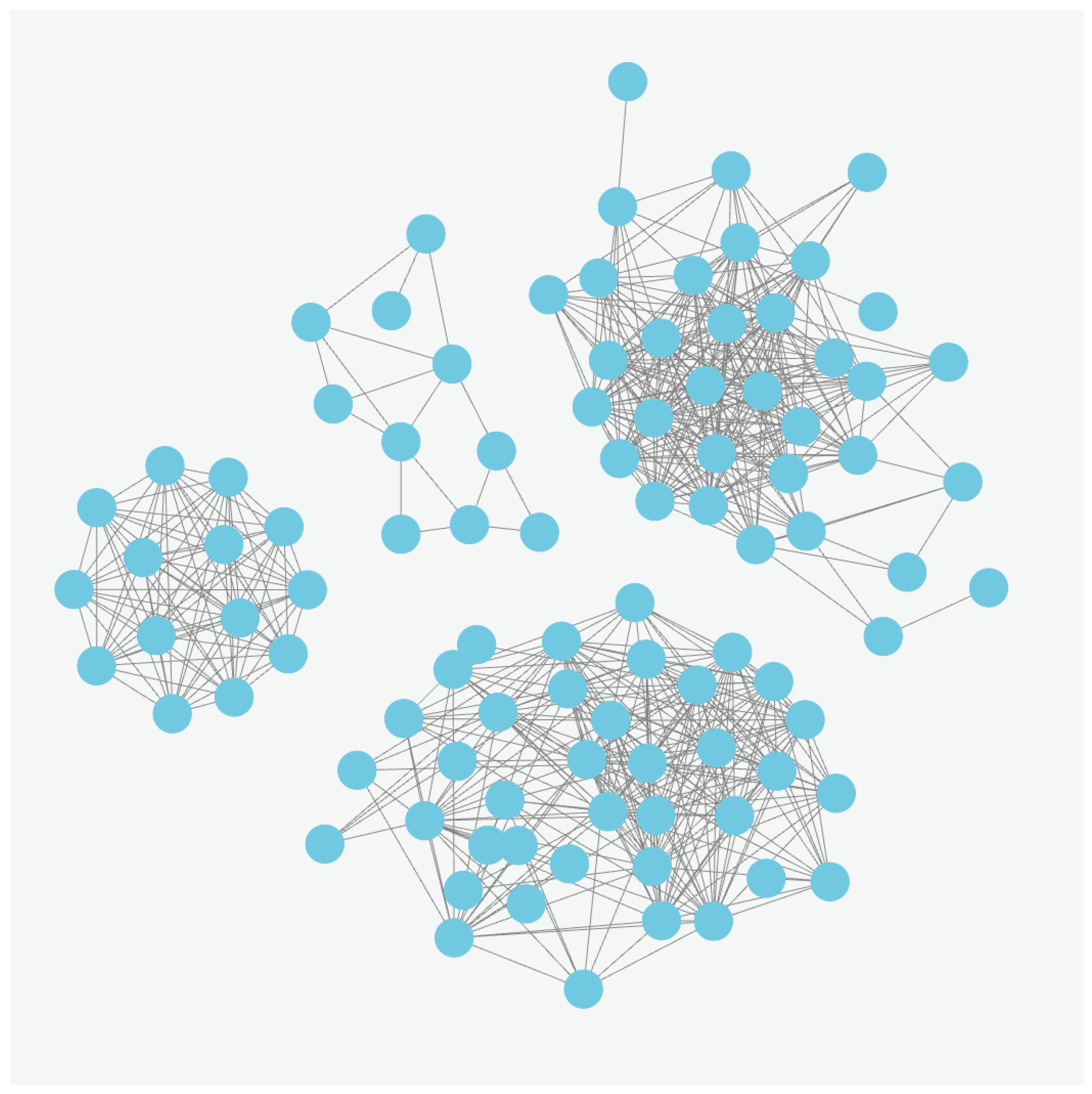
Using the Neo4j interactive tool, we have queried the database to display all epigrams and the similarity relationships between them with a similarity score of at least $0.9$. The outcome of this query is displayed in Figure 7, where we can clearly distinguish four different groups of nodes representing epigrams. In order not to cloud the image, nodes that are not connected to any of the four groups of nodes have been omitted. These outliers represent epigrams for which the text is barely known and, as such, do not display a high similarity with the epigrams that are part of a node group after executing the query. Upon closer examination of the query results, we observed that the leftmost group of nodes predominantly corresponds to the original group of four-verse epigrams. The bottom group of nodes relates to the original group of three-verse epigrams, and the rightmost group of nodes primarily corresponds to the original group of two-verse epigrams.

Upon further investigation, it becomes evident that the sparsely connected group of nodes in the middle of the image also comprises epigrams associated with the original group featuring two-verse epigrams. The epigrams in this fourth node group exhibit a common variation compared to the other two-verse epigrams. This variation is substantial enough that the similarity scores between the epigrams from these distinct node groups fall below the specified threshold of $0.9$. 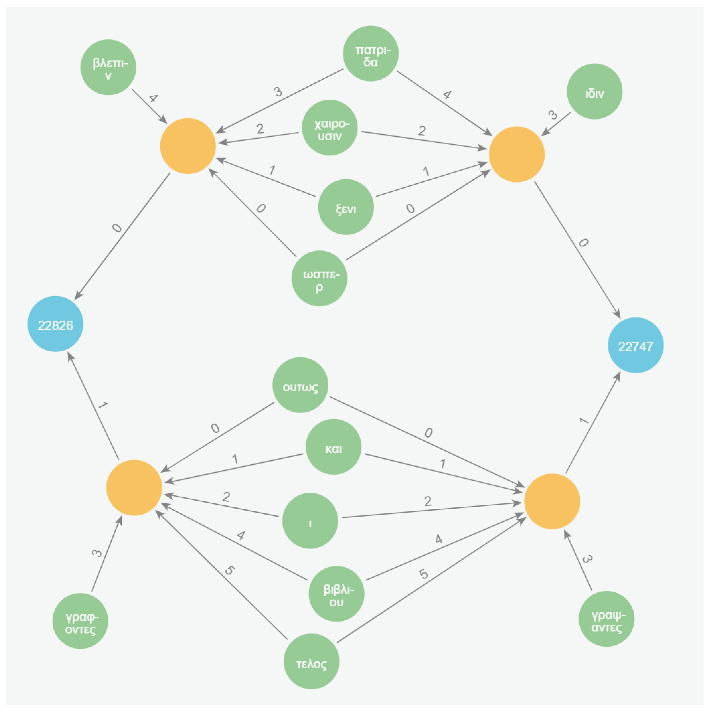Neo4j’s interactive environment facilitates a detailed investigation by allowing us to expand the epigram nodes into their hierarchical components. Figure 8 shows the expanded view of an epigram from this fourth node group (left) and an epigram from the other node group representing the two-verse epigrams (right).

This image reveals a subtle spelling variation in a word within the verses ranked 1. A more significant variation occurs in the verses ranked 0, where the last two words are swapped, and the left epigram uses the word βλεπιν instead of ιδιν, which are synonymous. Upon examining other epigrams from both groups, it becomes apparent that this larger variation in the first verse distinguishes the original group of two-verse epigrams into two separate groups of nodes.

This example demonstrates a potential application for the proposed graph model when implemented in a graph database system. The visual and interactive query capabilities of a graph database, paired with the proposed graph model, provide an ideal research tool for exploring and analysing (the connections within) a given corpus or computing graph-based statistics on textual data. Furthermore, by delving into the underlying structure of the texts and the similarities among these smaller text elements, the overall similarity score between two entire text documents becomes more interpretable compared to a similarity measure calculated solely on a sequence of characters and/or tokens.

7. Conclusions and Future Work

In this paper, we proposed a novel orthographic similarity measure designed for handling interconnected texts. We began by discussing the hierarchical decomposition of texts into textual components based on the discourse units within a given textual corpus. We then proposed a graph-based text representation where different types of nodes correspond to different discourse units of such a hierarchical decomposition, where the smallest textual elements are represented by nodes storing the actual textual data. Higher-level textual elements are represented by subgraphs, where the original text can be reconstructed by traversing down to the smallest textual components. By representing the identical textual content with a single node, a basic notion of similarity between texts can be deducted from the resulting graph structure.

Building on this graph representation, we proposed a method for hierarchically computing pairwise similarity scores between all textual components on the same level of the graph. This procedure, which found its origin in edit distances between strings, starts by determining pairwise string-based similarity scores between the lowest-level text elements. As a novelty, the pairwise similarities between higher-level nodes with the same label are hierarchically computed using a node-based edit distance that incorporates the precomputed similarity values between lower-level nodes. This hierarchical procedure is repeated until the similarity between the top-level elements, representing entire text documents, are determined.

The resulting graph-based text representation, along with the computed similarity scores, opens up avenues for developing novel text analysis or mining applications that leverage the structural information of texts and the similarities among text components. Since the intermediate similarity scores are also stored in the graph, the computation of the overall similarity scores can be easily interpreted and therefore contributes to the explainability of artificial intelligence applications using this measure. Moreover, the resulting graph can be implemented in a graph database system, enabling flexible and nuanced queries for textual analysis as well as the computation of graph-based statistics on texts.

The usefulness and performance of these novel techniques were determined by means of a corpus of Byzantine book epigrams, showcasing effectiveness on highly interconnected and orthographically inconsistent texts. A quantitative analysis demonstrated the proposed technique’s performance on these complex texts as well as how they relate to a state-of-the-art soft similarity measure, only considering two levels of textual components. Additionally, a hands-on example illustrated the similarity measure’s potential as a research tool for visually and interactively analysing textual data and the connections among them. As the methods proposed in this paper aim to handle texts by leveraging their underlying structure, it serves as an initial step toward establishing a framework for handling unstructured texts in a semi-structured manner.

Given its orthographic and highly customisable nature, this approach extends beyond Byzantine book epigrams and can also be applied to analyse other short textual documents, such as, abstracts, lyrics or short product descriptions, as well as texts written in different languages. This technique can later be extended and tested to handle larger types of text documents.

In future work, we plan to explore the extension of this hierarchical similarity measure to other orthographic or semantic measures. When different similarity scores between nodes are stored in the graph, we will also investigate methods to aggregate two or more of these measures in the hierarchical computations or in flexible queries. Furthermore, we will investigate existing new text mining techniques, including clustering or classification methods, and asses how they can be adapted to leverage this innovative hierarchical similarity measure.