OptimSolution: A Cross-Platform Framework for Benchmarking, Sensitivity, and Complexity Analysis of Continuous Optimisation Methods

Abstract

We present OptimSolution, an open-source, cross-platform framework for the systematic benchmarking and analysis of continuous optimisation methods, available for Windows, Linux and macOS and operable via both a command-line interface (CLI) and a Qt-based Graphical User Interface (GUI). The framework supports four execution modes: Single mode for single method–problem runs with convergence and distribution analysis; Batch mode for automated multi-method, multi-problem experimentation with aggregated statistical summaries; Method Sensitivity Analysis for quantifying the effect of algorithmic hyperparameters on solution quality; and Problem Sensitivity Analysis for assessing how problem-defining parameters influence instance difficulty and inter-method rankings. Complexity analysis is provided along two-axes method scalability across problem dimensionalities and problem difficulty profiles across method portfolios. Statistical validation is embedded natively through Wilcoxon signed-rank and Friedman tests with post-hoc pairwise analysis, complemented by rank tables and box-plot visualisations. All outputs are exportable as CSV files or publication-ready PNG figures. The framework is designed for extensibility: new methods and benchmark problems can be registered and activated through the GUI without modifications to the core codebase, supporting rapid experimental iteration.

1. Introduction

Continuous optimisation constitutes one of the most extensively studied areas in computational mathematics and computer science, encompassing problems in which a real-valued objective function must be minimised or maximised over a continuous search space, typically subject to bound or equality constraints. The practical difficulty of such problems arises from properties such as multimodality, non-convexity, high dimensionality, and the absence of analytical gradient information, which render exact methods computationally intractable in many real-world scenarios [1]. Over the past three decades, metaheuristic algorithms have emerged as a widely adopted class of approximate solvers capable of exploring large, complex search spaces without relying on derivative information. Seminal contributions in this class include the Genetic Algorithm (GA) [2], Particle Swarm Optimisation (PSO) [3], and Differential Evolution (DE) [4], alongside a steadily expanding body of variants and hybrid approaches, each proposing improvements in convergence speed, solution quality, or robustness.

The proliferation of metaheuristic methods has, however, introduced a parallel challenge: the rigorous, fair, and reproducible evaluation of algorithmic performance. Benchmarking an optimisation algorithm is a non-trivial undertaking that requires careful attention to experimental design, the selection of representative test problems, the choice of performance metrics, the number of independent runs, and the application of appropriate statistical tests [5]. In practice, inconsistent benchmarking protocols lead to results that are difficult to reproduce, compare, or generalise across studies [6]. Sensitivity of algorithm performance to hyperparameter settings, and the dependence of relative algorithm rankings on problem instance characteristics, further complicate the interpretation of benchmarking outcomes [7]. These concerns have motivated calls within the optimisation community for standardised, transparent, and tool-supported benchmarking workflows.

Several software frameworks have been developed to address aspects of this challenge. COCO [8] provides a black-box benchmarking environment with automated post-processing, IOHprofiler [9] offers a web-based interface for profiling iterative heuristics, Nevergrad [10], pymoo [11], MEALPY [12], NiaPy [13], opfunu [14], OPTIMUS [15], and GLOBe [16] each contribute algorithmic libraries and varying degrees of experimental support. Nevertheless, as detailed in Section 2, none of these tools combines a native desktop Graphical User Interface (GUI) with command-line operation, built-in Method and Problem Sensitivity Analysis, algorithmic complexity analysis across both methods and problem dimensions, embedded non-parametric statistical testing, and in-GUI extensibility for new methods and problems all within a single, cross-platform, self-contained framework.

This paper presents OptimSolution, an open-source framework for the systematic benchmarking and multi-faceted analysis of continuous optimisation methods. An earlier, undocumented prototype is publicly accessible at https://github.com/charilog/optimsolution (accessed on 28 June 2026); the present work constitutes its first formal description and introduces a substantially extended feature set. The framework is operable via both a Qt-based GUI and a CLI, and runs natively on Linux, Windows, and macOS. It supports four execution modes: Single (includes complexity analysis), Batch, Method Sensitivity Analysis, and Problem Sensitivity Analysis. Statistical validation via Wilcoxon signed-rank [17] and Friedman tests [18] is integrated natively, and all results are exportable as structured CSV files or publication-ready PNG figures. A key design objective is extensibility: new optimisation methods and benchmark problems can be registered through the GUI without modifying the core codebase.

The remainder of this paper is organised as follows. Section 2 reviews existing related frameworks and identifies the gaps that motivate this work. Section 3 describes the overall architecture and design of OptimSolution, covering the system architecture, installation procedure, extensibility mechanism, and additional framework features including termination criteria, initialisation strategies, and parallel methods. Section 4 presents the execution modes and analysis features in detail, including Single mode, Batch mode, sensitivity analysis, and GUI execution performance. Section 5 draws conclusions and outlines directions for future work.

2. Related Work

Several software frameworks have been developed to support the benchmarking and analysis of continuous optimisation methods, each addressing a distinct subset of the requirements identified in Section 1.

COCO version 1.0 [8] is a widely adopted black-box benchmarking platform that automates the comparison of continuous optimisers across standardised problem suites (BBOB), with automated post-processing and performance visualisation. However, it provides no GUI, no sensitivity analysis, and no in-framework statistical testing.

IOHprofiler version 0.3.22 offers a web-based interface for profiling iterative optimisation heuristics, supporting convergence tracking and performance analysis via its companion tool IOHanalyzer. Extensibility requires direct code modification, and sensitivity and complexity analyses are absent.

Nevergrad version 1.0 is a Python-based gradient-free optimisation platform developed at Meta Research, providing a broad collection of algorithms within a unified ask-and-tell interface. It offers no GUI, no sensitivity analysis, and no embedded statistical tests.

Pymoo version 0.6.2 is a Python framework focused on multi-objective optimisation, offering convergence visualisation and a partial hyperparameter sensitivity module. It requires manual scripting for Batch experiments and provides no statistical testing layer.

MEALPY version 3.0.3 is an open-source Python library consolidating a large number of metaheuristic algorithms. It supports Single runs and convergence tracking but lacks Batch automation, sensitivity analysis, and statistical validation.

NiaPy version 2.6.1 is a Python microframework designed to simplify the implementation and comparison of nature-inspired algorithms. It supports the basic export of results but provides no convergence plots, no statistical tests, and no analysis modes beyond individual runs.

Opfunu version 1.0.4 is a Python library providing a comprehensive catalogue of benchmark functions, including CEC competition suites. It functions exclusively as a problem repository and does not constitute a benchmarking or analysis framework.

OPTIMUS version 1.0.0 is a C++ command-line solver supporting multiple global optimisation methods with a plugin-based extensibility mechanism. It provides no GUI, no sensitivity or complexity analysis, and no statistical testing.

GLOBe version 1.0 is a recent modular C++/Python framework grounded in a formal mathematical unification of global optimisation algorithms. It consolidates classical and state-of-the-art methods within a family-level plugin architecture and includes an integrated benchmarking engine with extensible metrics. However, it offers no GUI, no sensitivity or complexity analysis, and no embedded non-parametric statistical tests.

Table 1. Comparison of continuous optimisation benchmarking frameworks with respect to key features. ✓ denotes full support, ~ partial or limited support, and ✗ no support.

Feature	OptimSolution	COCO/BBOB	IOHprofiler	Nevergrad	Pymoo	MEALPY	NiaPy	Opfunu	OPTIMUS	GLOBe
Language	C++/Qt	C/Python	C++/R	Python	Python	Python	Python	Python	C++	C++/Python
Platform	Linux, Win, Mac	Linux, Win, Mac	Linux, Win, Mac	Linux, Win, Mac	Linux, Win, Mac	Linux, Win, Mac	Linux, Win, Mac	Linux, Win, Mac	Linux, Win, Mac	Linux, Win, Mac
GUI	✓	✗	~	✗	✗	✗	✗	✗	✗	✗
CLI	✓	✓	✓	~	✗	✗	✗	✗	✓	✗
Single run	✓	✓	✓	✓	✓	✓	✓	~	✓	✓
Batch mode	✓	✓	✓	✓	~	~	~	✗	~	✓
Sensitivity (method)	✓	✗	✗	✗	~	✗	✗	✗	✗	✗
Sensitivity (problem)	✓	✗	✗	✗	✗	✗	✗	✗	✗	✗
Complexity analysis	✓	~	✗	✗	✗	~	✗	✗	✗	✗
Convergence plot	✓	~	✓	~	✓	✓	✗	✗	✗	✗
Distribution plot	✓	~	~	~	~	✗	✗	✗	✗	✗
Statistical tests	✓	~	✓	✗	✗	✗	✗	✗	✗	✗
Export CSV/PNG	✓	✓	✓	~	~	~	~	✗	~	~
GUI extensible	✓	✗	~	✗	✗	✗	✗	✗	~	~
Random benchmarks	✗	~	✗	✗	✗	✗	✗	✗	✗	✓
Python API	✗	✓	~	✓	✓	✓	✓	✓	✗	✓

summarises the features of the frameworks reviewed above in comparison with OptimSolution. As the table shows, no existing tool combines a native desktop GUI with CLI operation, four execution modes, Method and Problem Sensitivity Analysis, complexity analysis across both methods and problems, embedded non-parametric statistical testing, and in-GUI extensibility all within a single cross-platform framework.

The partial-support entries (denoted ~) in Table 1 reflect the following documented feature limitations. For COCO/BBOB: complexity analysis is partially supported through a dedicated CPU timing experiment that estimates per-evaluation cost and implicitly profiles ERT across fixed budget values, but no explicit scalability plots across problem dimensionalities or inter-method difficulty profiles are produced, convergence plots take the form of ECDF runtime distributions rather than per-run objective-value trajectories, distribution plots correspond to runtime ECDFs rather than box plots of final solution values, statistical comparison is limited to ERT-based ranking without embedded non-parametric tests such as Wilcoxon signed-rank or Friedman, and random benchmark support refers to randomly transformed instances of fixed BBOB base functions rather than dedicated random function generators such as GKLS. For IOHprofiler: the GUI is a web-based Shiny interface (IOHanalyzer) requiring an R runtime and browser access rather than a native desktop application, distribution plots visualise fixed-target runtime distributions rather than box plots of final objective values, extensibility requires modification of IOHexperimenter source code, and the Python API covers only the experimentation module (IOHexperimenter) while the analysis backend (IOHanalyzer) is implemented in R. For Nevergrad: CLI operation is available only as a Python module invocation (python -m nevergrad.benchmark) rather than a standalone executable, convergence plots and distribution plots are generated by separate post-processing scripts rather than interactively during or after a run, and CSV/PNG export requires invoking the post-processing pipeline rather than a single export action. For pymoo: method sensitivity analysis is partially supported since version 0.6.0 through a HyperparameterProblem formulation that treats hyperparameter tuning as an optimisation problem, but systematic parameter sweeps with statistical summaries (mean, SD, rank, main effect) require manual scripting, Batch mode and result export similarly require user-scripted experiment loops. For MEALPY: the Multitask class enables execution of multiple algorithms across multiple problems with optional parallel workers, but automated aggregated statistics and ranking tables are not produced, complexity (scalability) testing is supported as a scripted use case but not as an automated analysis mode, and per-run output files are generated in CSV and PNG formats, although aggregated comparative summaries require post-processing. For NiaPy: result export is limited to basic per-run data, convergence plotting is not natively supported and requires external scripting, as confirmed by the project’s own issue tracker.

3. Architecture and Design of OptimSolution

3.1. System Architecture

OptimSolution is implemented in ISO C++17 and organised into two principal components: a platform-independent core library (optimcore) and a Qt6-based graphical front-end. The CLI executable links directly against optimcore and is built independently of the GUI, enabling headless execution on server environments. The build system is CMake (≥3.16), which manages both targets through a unified configuration. The core library is structured into four layers. The problem layer provides a catalogue of benchmark and real-world continuous optimisation problems, currently comprising 92 instances. These include classical analytical functions such as Sphere, Rastrigin [19], Rosenbrock [20], Ackley [21], Griewank, Levy, Schwefel, Michalewicz, Zakharov, Bohachevsky, Camel, Easom, Shubert, Hansen, Gallagher, and Weierstrass (all documented in the comprehensive survey by Jamil and Yang [22]), the full CEC 2022 benchmark suite [23], GKLS random function instances [24], the complete CEC 2011 suite of real-world optimisation problems [25], and additional engineering design problems covering antenna array synthesis, heat exchanger design, economic load dispatch, transmission network expansion planning, and kinematic inverse problems, among others. In its current version (v51), OptimSolution addresses unconstrained and bound-constrained continuous optimisation problems exclusively, support for problems with nonlinear equality or inequality constraints is identified as a direction for future work (Section 5). The method layer currently includes 67 optimisation algorithms. Population-based metaheuristics comprise Differential Evolution, Particle Swarm Optimisation (PSO), GA, Covariance Matrix Adaptation Evolution Strategy (CMA-ES) [26], Whale Optimisation Algorithm (WOA) [27], Grey Wolf Optimiser (GWO) [28], Artificial Bee Colony (ABC) [29], Simulated Annealing (SA) [30], Ant Colony Optimisation for continuous domains [31], Teaching–Learning-Based Optimisation (TLBO) [32], Jaya [33], Sine Cosine Algorithm (SCA) [34], Firefly Algorithm (FA) [35], Bat Algorithm (BA) [36], Harmony Search (HS) [37], Cuckoo Search (CS) [38], Slime Mould Algorithm (SMA) [39], Marine Predators Algorithm (MPA) [40], Equilibrium Optimiser (EO) [41], Harris Hawks Optimisation (HHO) [42], Moth-Flame Optimisation (MFO) [43], Ant Lion Optimiser (ALO) [44], Water Cycle Algorithm (WCA) [45], Krill Herd (KH) [46], and Honey Badger Algorithm (HBA) [47], among others. State-of-the-art competition variants include jSO [48], mLSHADE-RL [49], NL-SHADE-LBC [50], and EA4eig [51]. Classical local search procedures comprise BFGS [52], L-BFGS [53], Nelder-Mead [54], and Gradient Descent. The analysis layer implements the execution modes described in Section 4, together with the statistical testing and output modules. The interface layer exposes all functionality through both the CLI and the Qt GUI. A factory pattern (factory.cpp) registers all methods and problems at compile time and serves as the single point of integration for new components, as described in Section 3.3.

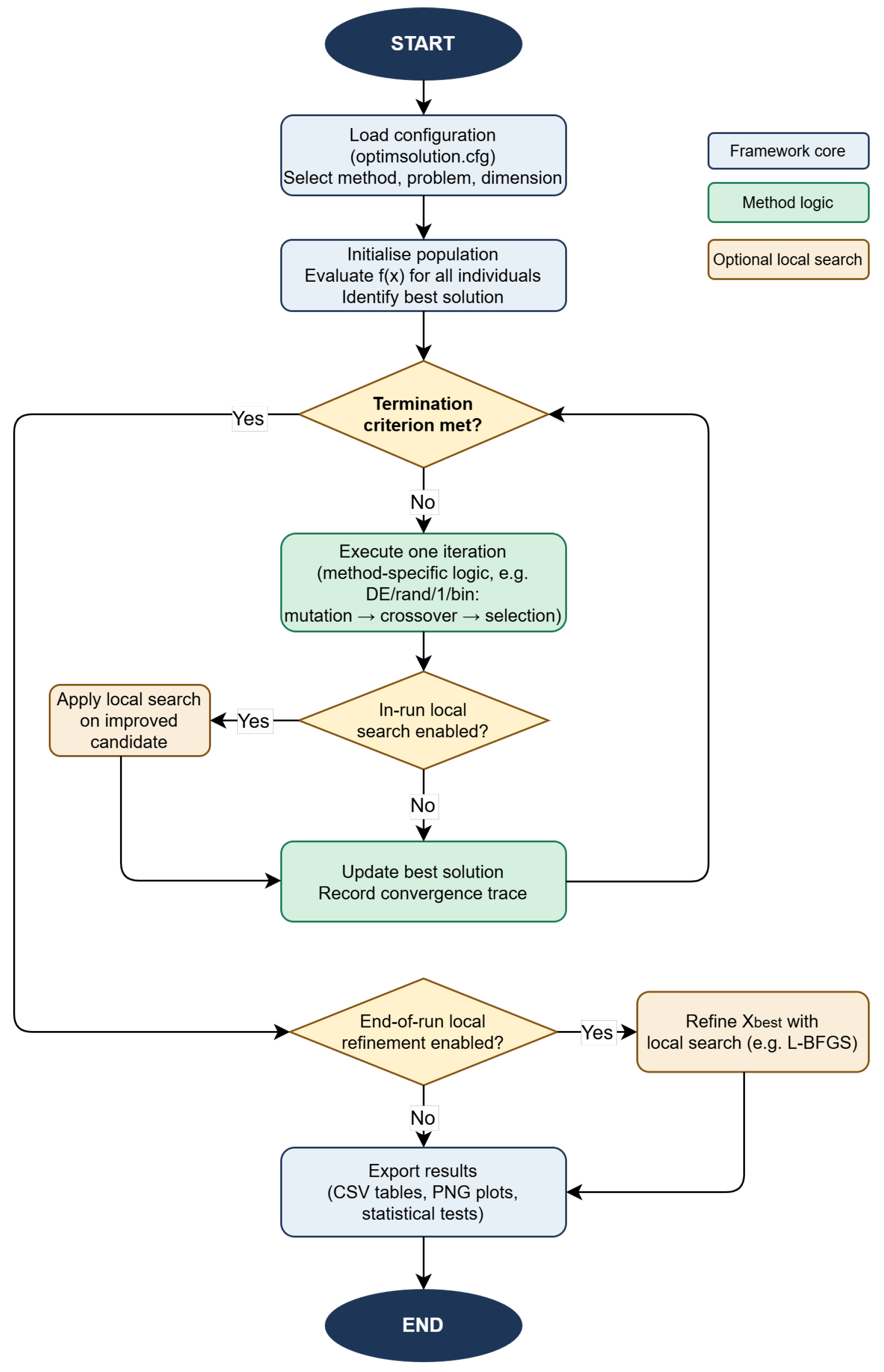
Figure 1 presents the general execution flow of OptimSolution. Upon loading the configuration file, the framework initialises the population and evaluates the objective function for all individuals. The main loop iterates until a termination criterion satisfies maximum function evaluations, maximum iterations, or a convergence-based stopping rule. Within each iteration, the method-specific optimisation logic is executed (for example, DE/rand/1/bin applies mutation, crossover, and greedy selection), and an optional in-run local search can be triggered probabilistically on improved candidates. Upon termination, an optional end-of-run local refinement polishes the best solution found before results are exported as CSV files and PNG figures.

3.2. Installation Procedure and Example Run (v51)

The source code is openly available at https://github.com/charilog/optimsolution (accessed on 28 June 2026) (release v51, commit 6dfcabc). A permanent archived snapshot is available via Zenodo at https://zenodo.org/records/20646845 (accessed on 28 June 2026). The version described in this paper is v51. The software requires a C++17 compliant compiler and CMake ≥ 3.16. The Qt6 library (https://qt.io (accessed on 28 June 2026)) is additionally required for compilation of the GUI target.

On Linux and macOS, after cloning the repository, the software is built with the standard CMake workflow:

cmake -S . -B build -G Ninja \   -DCMAKE_BUILD_TYPE=Release \   -DCMAKE_PROJECT_INCLUDE=cmake/optimsolution_gui.cmake cmake --build build --target optimsolution_gui cmake --build build --target optimsolution ./build/optimsolution_gui ./build/optimsolution arq tersoffc

Both the CLI executable (optimsolution) and the GUI application are produced in the build directory.

On Windows, the same CMake procedure applies when Qt6 and a compatible compiler (MSVC or MinGW) are available.

cmake -S . -B build -G "Visual Studio 17 2022" -A x64 ‘   "-DCMAKE_PROJECT_INCLUDE:FILEPATH=$PWD/cmake/optimsolution_gui.cmake" ‘   "-DCMAKE_PREFIX_PATH=C:\Qt\6.10.1\msvc2022_64" cmake --build build --config Release --target optimsolution_gui cmake --build build --config Release --target optimsolution & "C:\Qt\6.10.1\msvc2022_64\bin\windeployqt.exe" ‘   --no-translations --compiler-runtime ‘   ".\build\Release\optimsolution_gui.exe"

Alternatively, a pre-compiled installer (OptimSolution.exe) is provided in the repository, which installs the GUI application without requiring the Qt library or a build toolchain.

3.3. Extensibility Mechanism

A central design objective of OptimSolution is the ability to register new optimisation methods and new benchmark problems without modifying the framework core and without requiring the user to interact with the build system manually. This is achieved through a GUI-driven code generation and build pipeline implemented in the CodeGenDialog module.

To add a new optimisation method, the user invokes the New Method wizard from within the GUI. The wizard collects the method’s short name, full name, C++ class name, and the definitions of its configurable parameters (name, type, default value, and description). It then automatically generates a conforming .h/.cpp skeleton, patches factory.cpp to register the new method under its short name, and updates CMakeLists.txt to include the new source file. The generated source files are immediately opened in an integrated Code Editor dialogue, where the user implements the algorithm logic. A one-click Build button invokes the CMake build pipeline from within the GUI and streams the compiler output to a log panel. An equivalent New Problem wizard handles the registration of new benchmark problems, additionally allowing the user to specify dimensionality constraints, search-space bounds, and the known global optimum value where available. Registered methods and problems can equally be removed through a Delete dialogue, which reverses the factory and CMake patches and deletes the corresponding source files. The complete extensibility workflow from specification to compilation is thus contained within the GUI and requires no manual editing of build or registration files.

Listing 1 illustrates the skeleton generated by the New Problem wizard for a user-defined objective function myproblem. The Problem base class handles bound management, function-evaluation counting, and optimum tracking, the user is required to implement only the Single virtual method evaluate_core. The generated header and source are immediately opened in the integrated Code Editor upon generation.

Architecturally, the core library is structured around three design patterns. A Factory pattern serves as the single registration point for all methods and problems, mapping short string identifiers to constructors at compile time, the code-generation pipeline patches this registry automatically, so no manual registration is required. A Template Method pattern governs the execution flow: a common base class implements the outer optimisation loop covering initialisation, iteration, termination checking, and result export while each algorithm subclass overrides only the method-specific update step. A Strategy pattern decouples orthogonal concerns such as termination criteria and population-initialisation distributions from the optimiser itself, allowing them to be selected and composed freely through the configuration file without modifying any algorithm code. Population state is stored in contiguous arrays for cache-friendly access.

Error isolation is an inherent property of the framework’s process architecture. All optimisation runs execute within the CLI subprocess, which the GUI manages as a separate QProcess, consequently, a runtime fault in a user-implemented method terminates the subprocess without affecting the GUI process. The GUI detects the abnormal exit via the process exit code, reports it in the run log, and remains fully operational. Any CSV result files written before the fault are preserved for partial analysis.

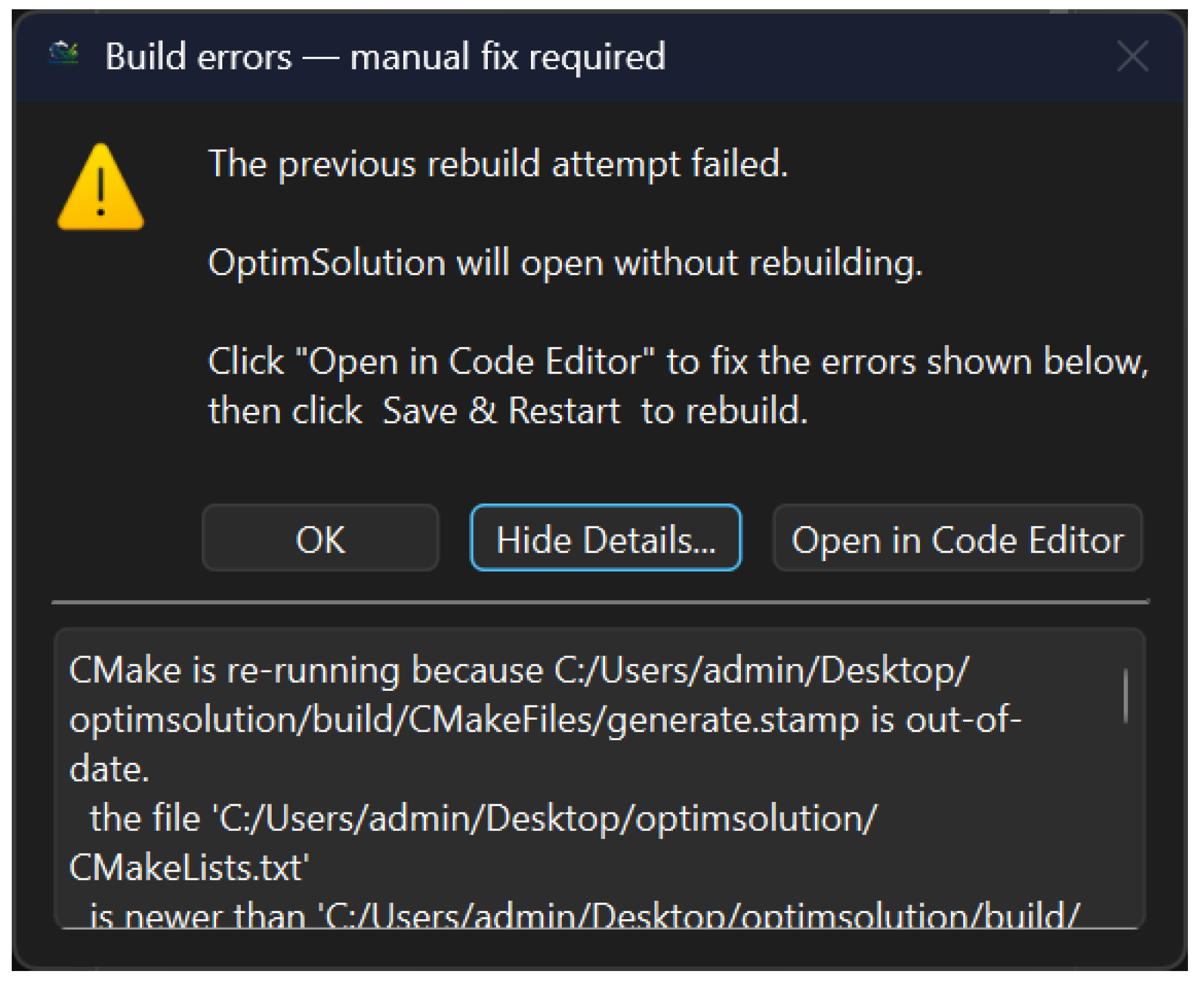
Compile-time errors in newly generated code are handled through a dedicated three-file recovery mechanism. When a new method or problem is generated, the wizard records the paths of the generated source files in a .rebuild_sources.txt marker alongside the .rebuild_pending flag. If the subsequent cmake build fails, the build script captures the full compiler output and writes it to .rebuild_errors.txt, then re-creates .rebuild_pending. On the next startup, the presence of both .rebuild_pending and .rebuild_errors.txt triggers a dedicated error-recovery dialogue (Figure 2) rather than the normal build prompt: the dialogue displays the compiler output, clears all three marker files, and, when the generated source files are still present on disk, offers an Open in Code Editor button that opens the integrated Code Editor pre-loaded with the correct source files and project root. The user corrects the errors directly in the editor and clicks Save & Restart, which re-creates the pending flag and initiates a fresh build cycle.

Listing 1. Auto-generated skeleton for a new benchmark problem (myproblem.h, myproblem.cpp)

// src/problems/myproblem.h - auto-generated #pragma once #include "problem.h" namespace optimsolution { class MyProblem : public Problem { public: MyProblem(); void init(int dim) override; protected: double evaluate_core(const Vec& x) override; // USER FILLS IN void gradient_core(const Vec& x, Vec& g) override; // optional }; } // namespace optimsolution ------------------------------------------------------- // src/problems/myproblem.cpp - auto-generated skeleton #include "myproblem.h" #include <cmath> namespace optimsolution { MyProblem::MyProblem() {     setName("myproblem");     setFullName("My Benchmark Problem"); } void MyProblem::init(int dim) {     Problem::init(dim);     Vec lo(dim, −5.12), hi(dim, 5.12);     setBounds(lo, hi); } // USER IMPLEMENTS THIS FUNCTION ONLY double MyProblem::evaluate_core(const Vec& x) {     // TODO: implement f(x).  Example: Sphere     double sum = 0.0;     for (double xi : x) sum += xi × xi;     return sum; } void MyProblem::gradient_core(const Vec& x, Vec& g) {     g.assign(x.size(), 0.0);     // TODO: implement gradient f(x) if gradient-based local search is desired } } // namespace optimsolution

3.4. Additional Framework Features

Termination criteria. OptimSolution provides ten configurable stopping rules, selectable through the configuration file. In addition to the standard maxevals (maximum function evaluations) and maxiters (maximum iterations) criteria, the framework implements the convergence-based rules bss, wss, tss, boss, srs, and irs, originally introduced and validated in [55], together with the doublebox criterion and an all rule that triggers termination as a logical disjunction of all active criteria halting execution as soon as any individual rule is satisfied. This composite stopping mechanism ensures an adaptive balance between convergence speed and solution accuracy across problem instances of varying difficulty.

Population initialisation strategies. The initialisation of the population is a critical factor affecting both the diversity of the initial search and the ultimate convergence behaviour of metaheuristic algorithms [56]. OptimSolution supports eleven initialisation distributions, selectable per experiment: uniform random sampling, normal, Cauchy, Laplace, log-normal, exponential, Beta, and Lévy distributions. It also supports three structured strategies: Latin Hypercube Sampling (LHS) [57], Halton low-discrepancy sequences, and oppositional initialisation. The k-means-based intelligent initialisation strategy proposed in [56] is also available, which uses a clustering-driven approach to generate initial estimates more closely aligned with the problem structure, thereby reducing the risk of premature convergence.

Parallel methods. OptimSolution includes natively parallel optimisation methods that exploit multi-core architectures via OpenMP. The Parallel Genetic Algorithm (PGA) [58] maintains a set of autonomous island sub-populations that periodically exchange their best solutions, combining the global exploration capabilities of the island model with the convergence guarantees of periodic migration. The Parallel Smell Agent Optimisation (PSAO) [59] extends the single-population SAO [60] with dynamic collaboration mechanisms and intelligent solution dispersal among sub-populations, accelerating global exploration while preventing premature convergence to local minima. Both methods are configurable through the standard configuration file and are subject to the same termination and initialisation options as all other framework methods.

4. Execution Modes and Analysis Features

4.1. Single Mode

Single mode executes a selected optimisation method on a selected problem for a configurable number of independent runs. The user specifies the method, problem, and problem dimensionality; all remaining parameters like population size, maximum function evaluations, number of runs, success tolerance, local search settings, and output options are read from a configuration file (optimsolution.cfg) shared between the CLI and the GUI. Each independent run is initialised with a distinct random seed derived from a common base seed, ensuring reproducibility while preserving stochastic diversity. At each run, the framework records the best objective function value as a function of function evaluations, producing a convergence trajectory. In the convergence plot, each line of the same colour corresponds to one independent run; the bundle of lines collectively characterises both the reliability of the method, i.e., the consistency of its convergence behaviour across repeated trials, and its validity, i.e., whether it systematically locates solutions of comparable quality, ideally close to the known global optimum. Upon completion, the descriptive statistics across all runs of best, worst, mean, standard deviation, and success rate are reported and optionally exported as CSV. A convergence curve plot and a box plot of the final solution values are generated and exportable as PNG.

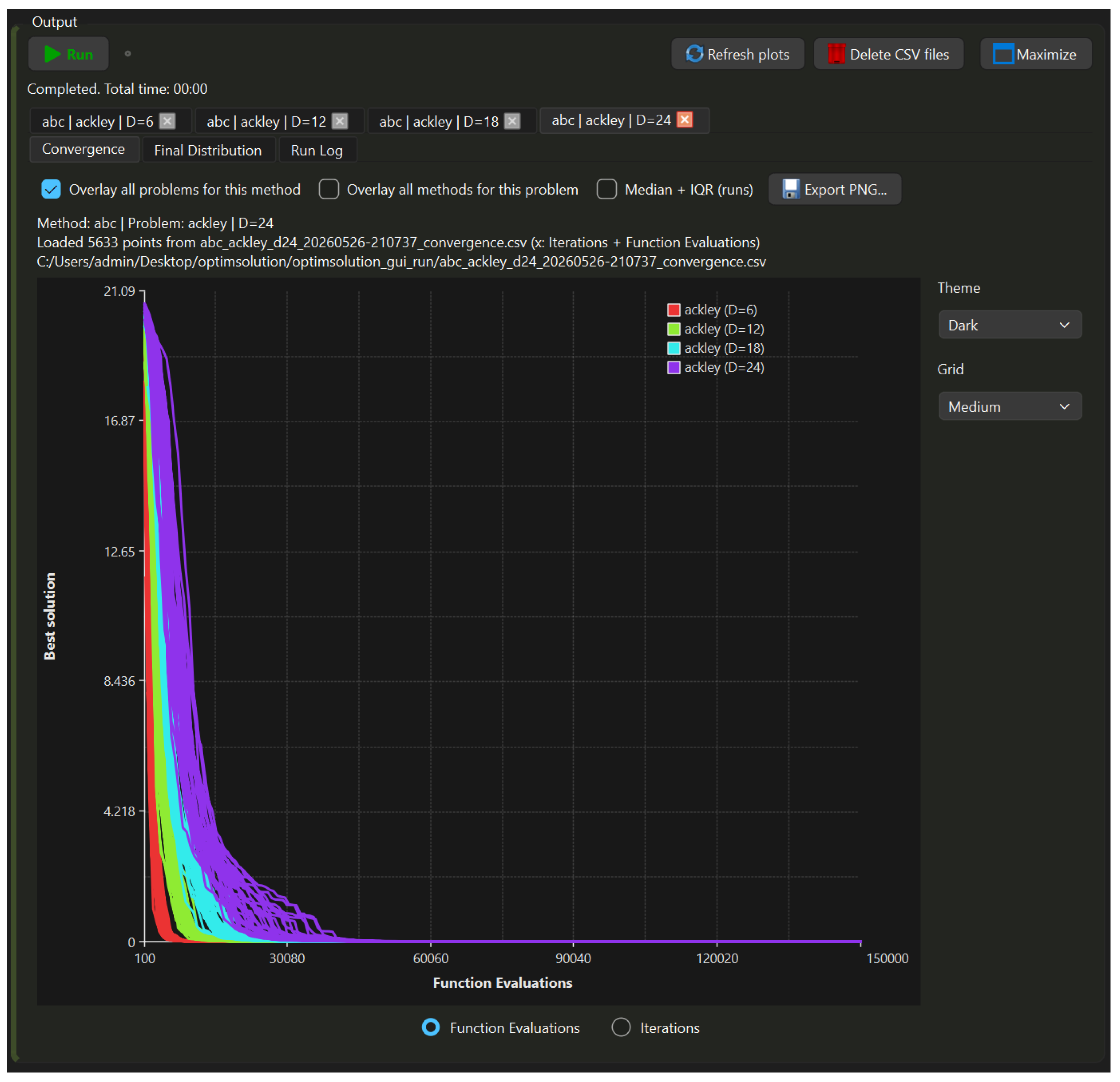
Single mode additionally supports complexity analysis through two overlay options available in both the GUI and the CLI. The first option overlays convergence curves across a set of user-defined dimensionalities for a fixed method–problem pair, characterising the scalability of the method as problem size grows. The second option overlays convergence curves across a set of methods for a fixed problem and dimensionality, producing a difficulty profile of the problem as seen by a method portfolio. Figure 3 illustrates an example of the first option: ABC applied to the Ackley function across the dimensions D = 6, 12, 18, and 24, where each colour corresponds to a different dimensionality and the spread of same-colour lines reflects run-to-run variability at that dimension.

4.2. Batch Mode

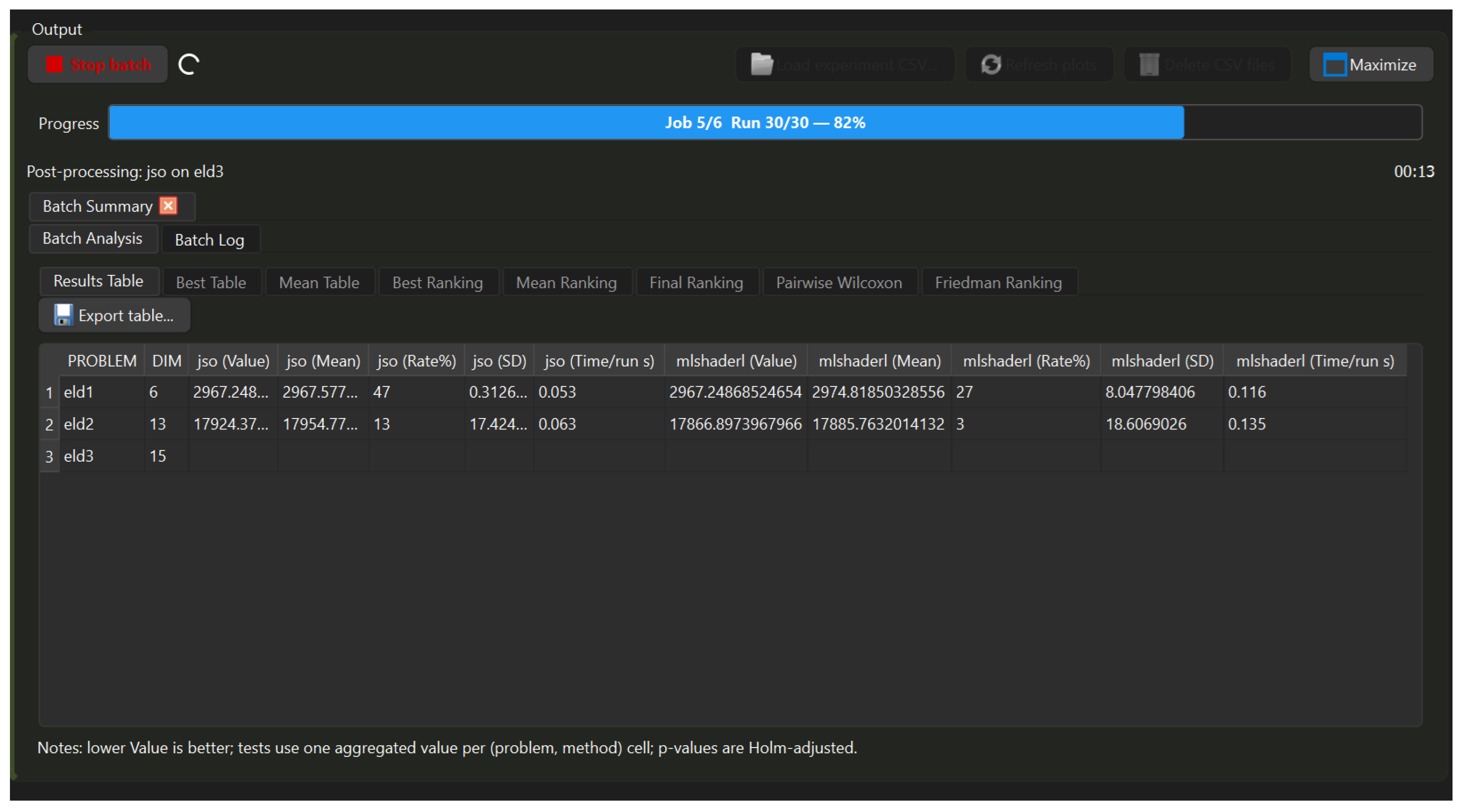
Batch mode automates the systematic evaluation of a user-defined set of methods across a user-defined set of problems. The framework executes every method–problem combination for the number of independent runs specified in the configuration file, processing all jobs sequentially and reporting progress in real time. Figure 4 illustrates an in-progress Batch experiment comparing jSO and mLSHADE-RL on the Economic Load Dispatch problems eld1, eld2, and eld3 [25] at the dimensions D = 6, 13, and 15, respectively. The results table displays, for each method–problem pair, the best value found across all runs, the mean, the success rate, the standard deviation, and the mean wall-clock time per run, enabling a direct quantitative comparison.

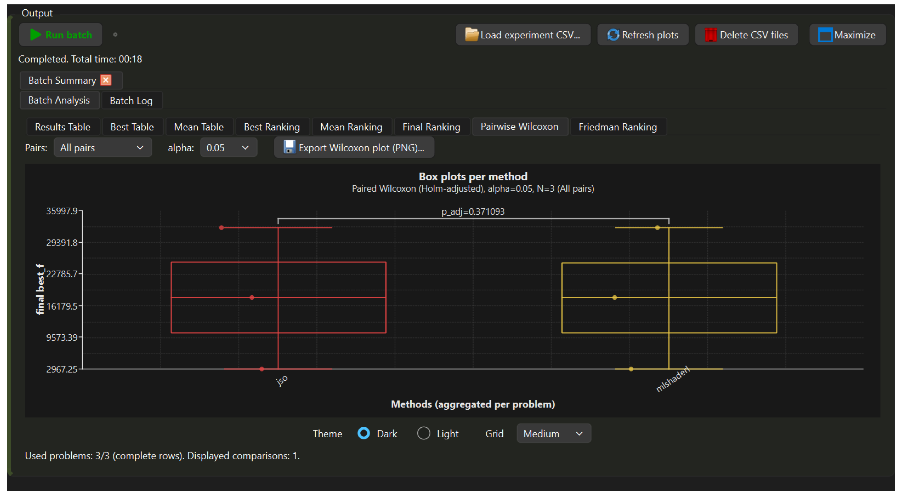
Upon completion, the Batch Analysis panel organises the results across eight views: Results Table, Best Table, Mean Table, Best Ranking, Mean Ranking, Final Ranking, Pairwise Wilcoxon, and Friedman Ranking. Figure 5 shows the Pairwise Wilcoxon view for the same experiment: box plots of the final best-value distributions are displayed for each method, aggregated across all three problems, with Holm-adjusted p-values annotated for each comparison. In this example, the comparison between jSO and mLSHADE-RL yields $p_{adj}$ = 0.371, indicating no statistically significant difference at $\alpha$ = 0.05. All tables and plots are exportable as CSV and PNG respectively.

4.3. Method and Problem Sensitivity Analysis

OptimSolution provides two complementary sensitivity analysis modes, accessible through dedicated run-mode selections in both the GUI and the CLI.

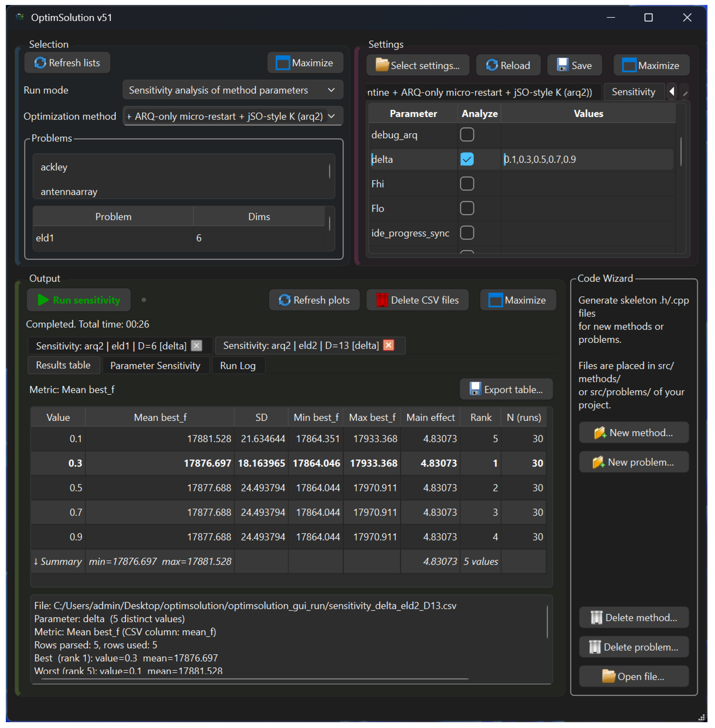
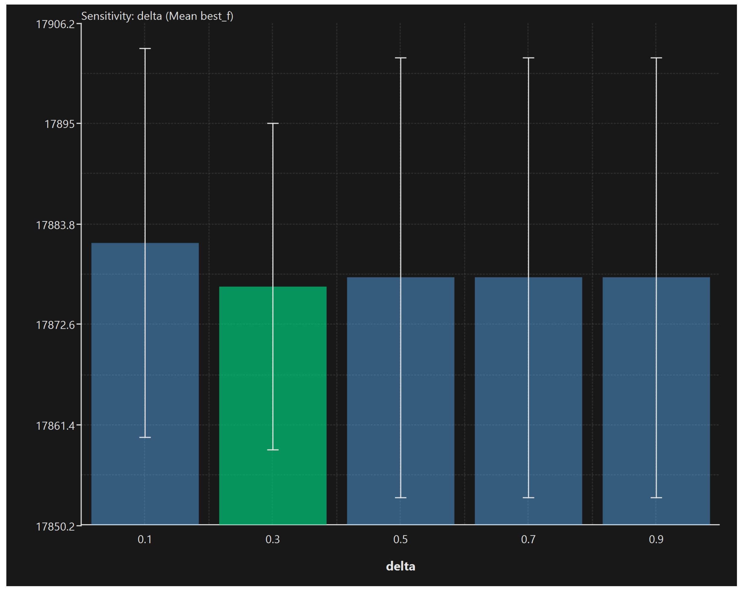
Method Sensitivity Analysis examines how variations in an algorithm’s own hyperparameters affect its performance on a selected set of problems. The user specifies the parameter of interest and the discrete values to evaluate through the Sensitivity panel of the Settings window, the framework then executes the method for each parameter value across all selected problems for the configured number of independent runs, and produces a Results table reporting, for each parameter value, the mean best objective value, standard deviation, minimum, maximum, main effect, rank, and number of runs. Figure 6 illustrates an example in which the parameter delta of ARQ2 [61,62] is swept over the values {0.1, 0.3, 0.5, 0.7, 0.9} on the Economic Load Dispatch problems eld1 (D = 6) and eld2 (D = 13). The table in Figure 6 highlights in bold the top-ranked configuration, here delta = 0.3 achieves the lowest mean best value on eld2 (mean $bes{t}_f$ = 17,876.697, rank 1). Figure 7 shows the corresponding bar chart for eld2, where each bar represents the mean best value with a 95% confidence interval and the green bar identifies the optimal parameter value, allowing the practitioner to distinguish robust from critical parameter regions.

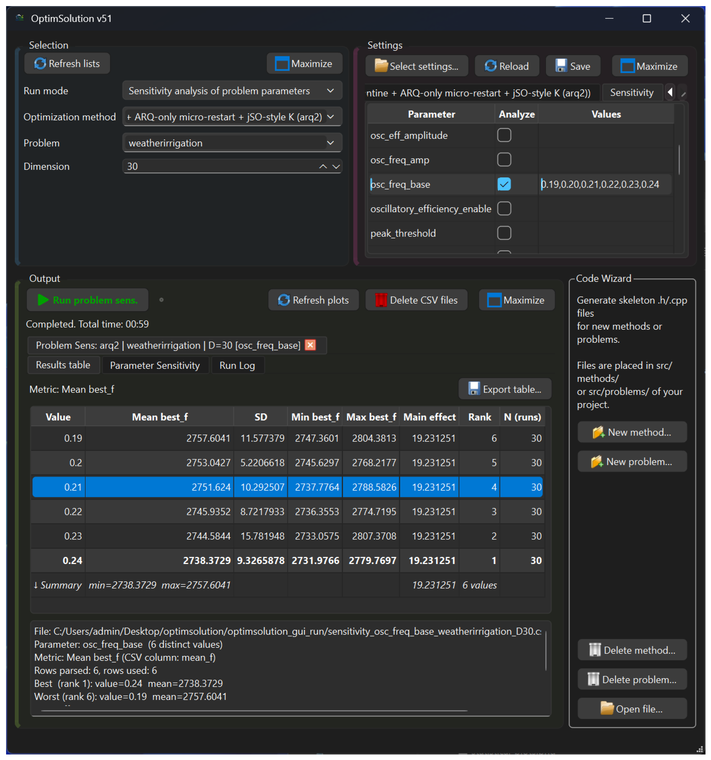
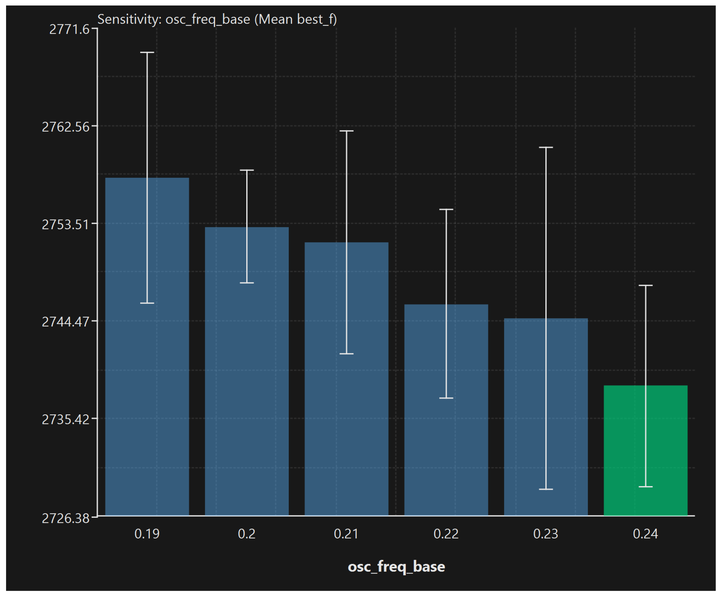
Problem Sensitivity Analysis examines how variations in a problem’s own defining parameters affect instance difficulty and the relative performance of a selected method. The user selects a problem, a method, and one or more problem parameters to sweep, the framework applies the method to each resulting problem instance and reports the same set of metrics. Figure 8 shows an example in which ARQ2 is applied to the weatherirrigation problem at D = 30, sweeping the parameter $os{c}_{fre\_base}$ over the values {0.19, 0.20, 0.21, 0.22, 0.23, 0.24}. The best-performing problem configuration is $os{c}_{fre\_base}$ = 0.24 (mean $bes{t}_f$ = 2738.37, rank 1), while the most difficult instance for this method is $os{c}_{fre\_base}$ = 0.19 (mean $bes{t}_f$ = 2757.60, rank 6). Figure 9 shows the corresponding bar chart, where the green bar identifies the parameter value that minimises the mean objective value. All results are exported as CSV and PNG.

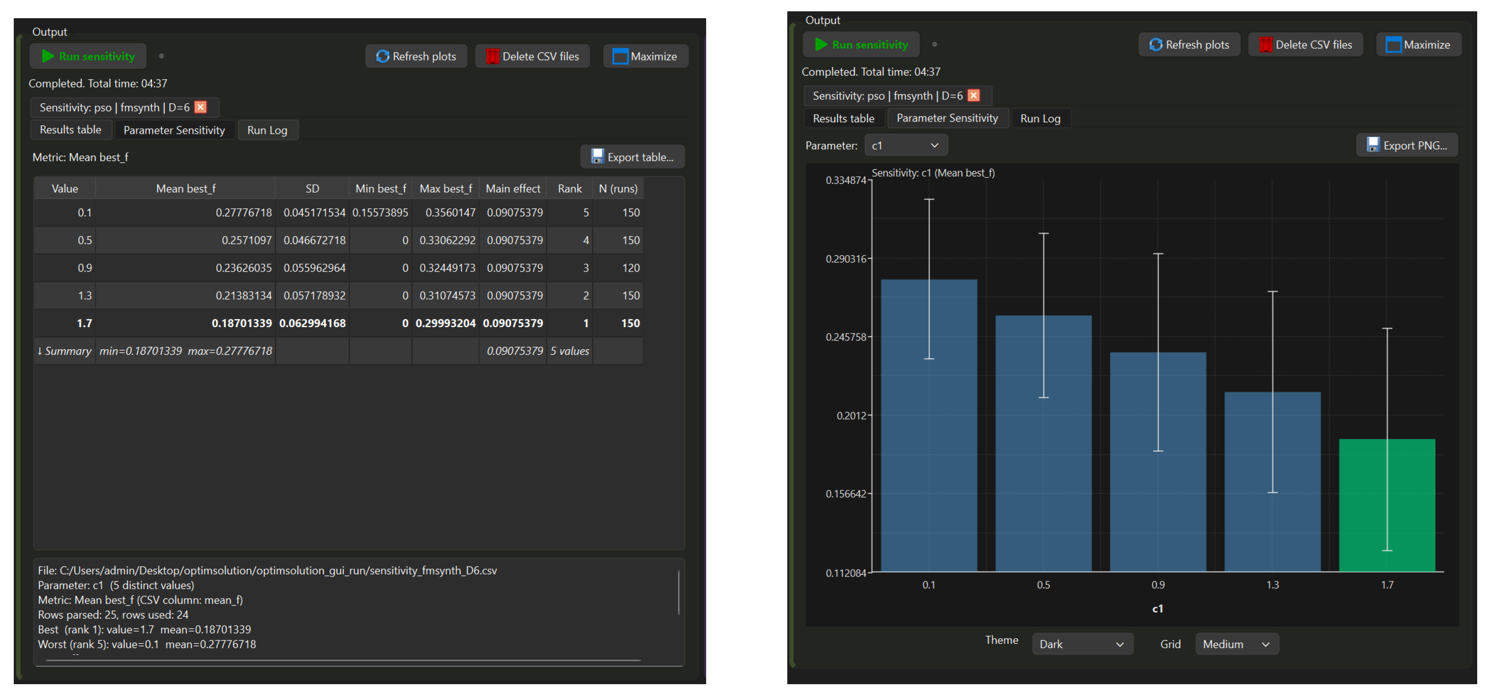
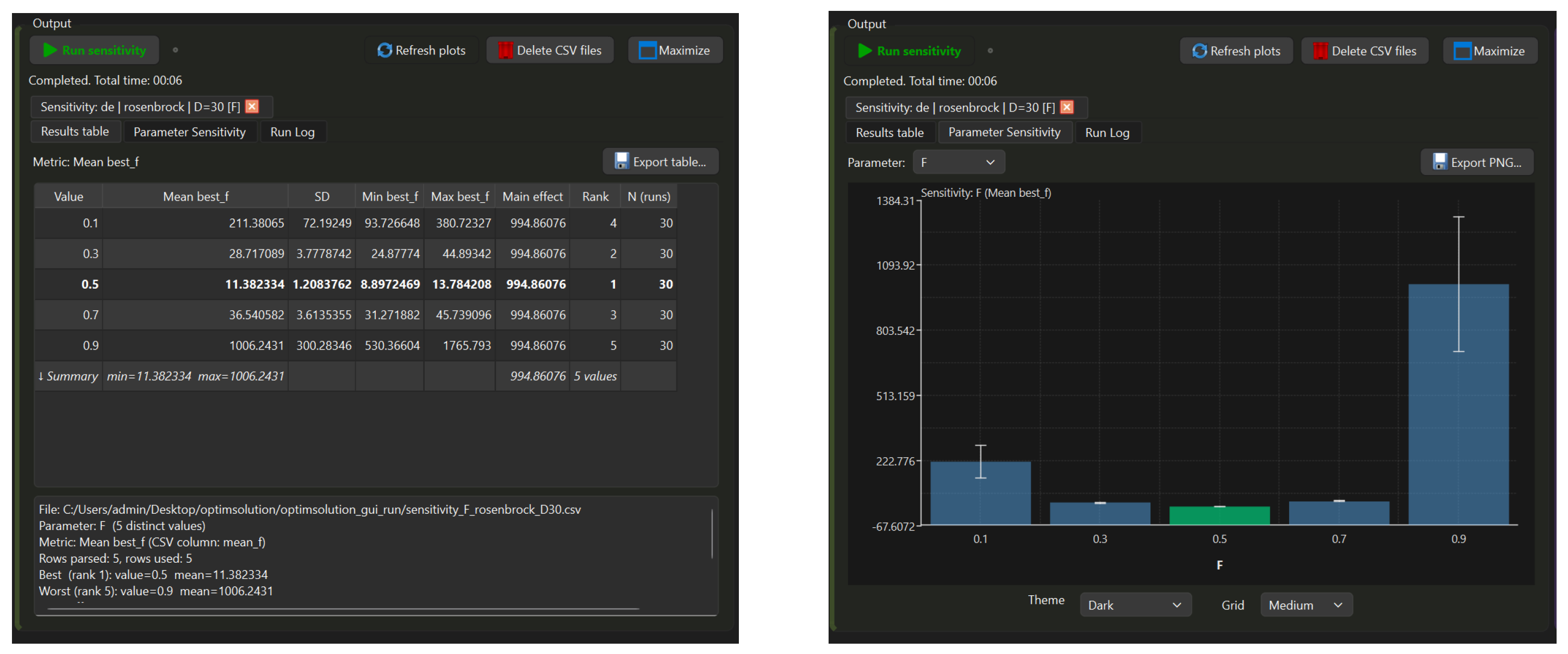
To demonstrate that the sensitivity analysis mode operates uniformly across fundamentally different algorithmic paradigms and is not specific to the ARQ family, two additional examples are presented. Figure 10 illustrates the sensitivity of PSO with respect to its cognitive acceleration coefficient $c_1$, swept over the values {0.1, 0.5, 0.9, 1.3, 1.7} on the FM Synthesizer Parameter Estimation problem (fmsynth, D = 6) over 150 independent runs. Performance improves monotonically as c₁ increases: $c_1$ = 1.7 achieves the lowest mean best value (mean best_f = 0.187, rank 1), while $c_1$ = 0.1 yields the weakest performance (mean best_f = 0.278, rank 5), indicating that stronger cognitive attraction consistently benefits PSO on this problem. Figure 11 presents the analogous experiment for Differential Evolution, sweeping the scale factor F over {0.1, 0.3, 0.5, 0.7, 0.9} on the Rosenbrock function (D = 30) over 30 independent runs. Here the relationship is non-monotonic: F = 0.5 achieves the lowest mean best value (mean best_f = 11.38, rank 1), while both extremes F = 0.1 (mean best_f = 211.38, rank 4) and F = 0.9 (mean best_f = 1006.24, rank 5) perform substantially worse, revealing a clear optimal operating region for this parameter.

4.4. GUI Execution Performance

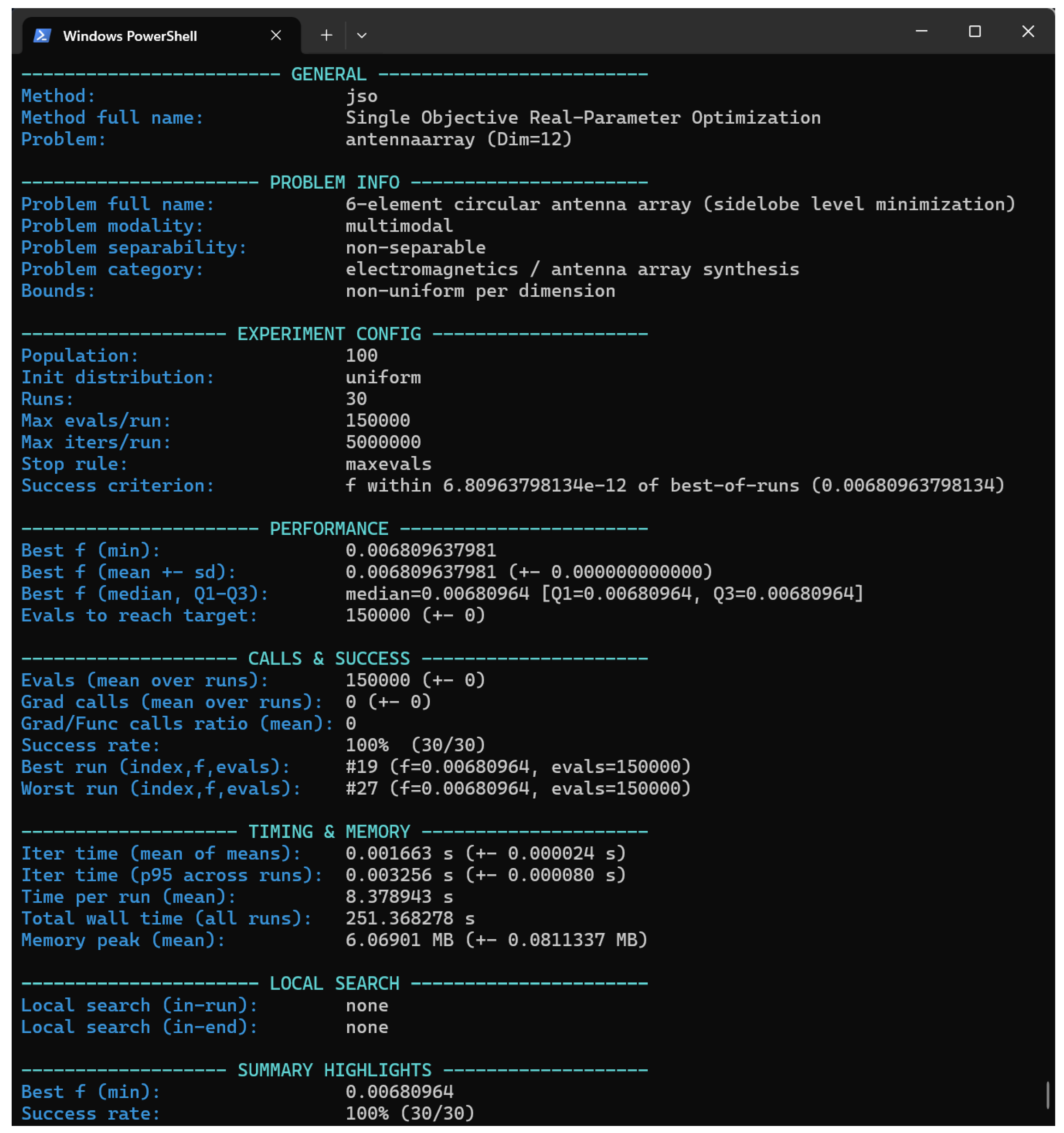
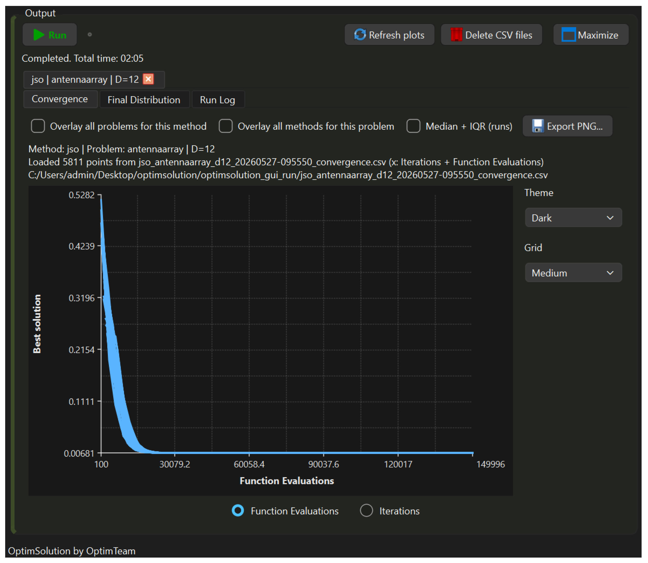
Although the GUI and the CLI share an identical computational core, the GUI achieves substantially lower wall-clock execution times on multi-run experiments when the CLI is used in its default mode with output directed to the terminal. To quantify this effect systematically, jSO was applied to the six-element circular antenna array synthesis problem [25] (D = 12) for 30 independent runs under identical configuration across three conditions: GUI, CLI with terminal output, and CLI with all outputs suppressed via PowerShell redirection (|Out-Null). As reported in the CLI summary (Figure 12), the mean time per run was 8.38 s, yielding a total wall-clock time of 251.37 s, with a best objective value of 0.00680964 and a 100% success rate across all 30 runs. The GUI completed the same experiment in 125 s (Figure 13), delivering an identical best objective value and convergence profile and a speedup factor of approximately $2.0\times$ over the default CLI. When CLI output was fully suppressed, the wall-clock time dropped to 125.23 s, statistically identical to the GUI. This result demonstrates that the $2.0\times$ speedup is attributable entirely to terminal I/O overhead in the default CLI mode: the GUI accumulates process output in an internal buffer and flushes it at fixed intervals rather than rendering each line in real time, effectively eliminating the overhead that dominates CLI wall-clock time when output is directed to the terminal. The underlying computational workload is identical in both interfaces.

It is important to clarify that the ~$2\times$ difference in wall-clock time does not reflect any computational speedup: the underlying workload is identical in both interfaces, as confirmed by the fact that when CLI output is fully suppressed (|Out-Null), both complete in statistically identical wall-clock time (~125 s). The observed difference under standard CLI execution is attributable solely to terminal I/O overhead, which the GUI reduces through three mechanisms. First, process output is not rendered in real time, it is accumulated in an internal buffer and flushed to the log panel at fixed intervals, preventing the graphical event loop from processing thousands of individual rendering events per second. Second, at each flush only a filtered subset of output lines is displayed, further reducing the UI update cost during long runs. Third, once a run completes, result parsing and statistical aggregation are performed concurrently on a background thread while the next run is already launching in the foreground, effectively pipelining computation and I/O.

Regarding GUI scalability for large-scale Batch experiments, the framework applies two complementary strategies. First, convergence data is downsampled to a maximum of 6000 points per run prior to rendering, using uniform stride sampling, this keeps the convergence plot responsive regardless of the number of function evaluations. Second, the live log panel is bounded by a 400,000-character circular buffer, with at most 60 lines displayed per flush cycle and the underlying Qt text document capped at 300,000 characters, preventing UI stalls during long multi-method runs. Box-plot visualisations in the Wilcoxon and Friedman panels are rendered from aggregated summary statistics rather than raw per-run data, so their rendering cost scales with the number of methods rather than the number of runs. No hard limit is imposed on the number of methods or problems in a Batch experiment; however, it should be noted that for very large method portfolios, typically beyond 50 methods, the exported box-plot images may suffer from visual degradation: individual boxes become narrow, labels overlap, and whiskers may occlude one another, reducing the readability of the figure. These are purely presentational artefacts of fixed-width image export, all underlying computed values means, medians, quartiles, Holm-adjusted p-values, and rankings remain numerically correct regardless of portfolio size. For such large-scale comparisons, users are therefore advised to rely on the exported CSV tables for quantitative analysis and to use the CLI for headless execution, post-processing the results with dedicated visualisation tools.

4.5. Correctness Validation

To verify that the algorithm implementations in OptimSolution produce results consistent with those reported in the original publications, three widely studied methods, DE, PSO, and CMA-ES, were applied to five classical benchmark functions: Sphere, Rastrigin, Rosenbrock, Ackley, and Griewank, all at dimension D = 30. Each method was executed for 30 independent runs with a population of 50 individuals and a budget of 150,000 function evaluations, using the standard parameter settings reported in the respective original papers: for DE, scale factor F = 0.5 and crossover rate $CR$ = 0.9, for PSO, inertia weight w = 0.729 and acceleration coefficients $c_1$ = $c_2$ = 1.496, for CMA-ES, initial step size $\sigma$ = 0.5.

Table 2. Validation of OptimSolution implementations against published reference results. Mean $f_{best}$ ± SD over 30 independent runs, D = 30, maxevals = 150,000.

Problem	DE Reference	DE OptimSolution	PSO Reference	PSO OptimSolution	CMA-ES Reference	CMA-ES OptimSolution
Sphere	0	0	$2.4\times {10}^{-5}$	0	0	0
	0	0	$1.1\times {10}^{-5}$	0	0	0
Rastrigin	45.3	16.461	89.4	52.602	8.2	0
	12.7	8.225	18.3	13.115	6.1	0
Rosenbrock	27.6	23.311	142.3	16.036	4.1	0.133
	14.2	1.433	67.4	1.813	3.8	0.728
Ackley	$3.2\times {10}^{-4}$	0	1.4	0.599	0	0
	$1.8\times {10}^{-4}$	0	0.8	0.777	0	0
Griewank	$2.1\times {10}^{-3}$	0.0045	0.08	0.014	0	0
	$1.4\times {10}^{-3}$	0.0102	0.04	0.018	0	0

reports the mean best objective value (mean $f_{best}$) and standard deviation (SD) obtained by OptimSolution alongside the corresponding reference values drawn from published benchmark studies [4,26,63]. The results confirm that OptimSolution’s implementations reproduce the published performance profiles within the expected range of stochastic variation, validating the correctness of the framework’s algorithmic core across three structurally distinct optimisation paradigms.

5. Conclusions

This paper presented OptimSolution, an open-source, cross-platform framework for the systematic benchmarking and multi-faceted analysis of continuous optimisation methods. The framework is operable via both a Qt-based GUI and a CLI, runs natively on Linux, Windows, and macOS, and provides a unified configuration layer that guarantees identical experimental conditions across both interfaces. The four execution modes Single, Batch, Method Sensitivity Analysis, and Problem Sensitivity Analysis, together with a complexity analysis module, cover the full spectrum of evaluation tasks required in modern metaheuristic research. Embedded non-parametric statistical testing via Wilcoxon signed-rank and Friedman tests with post-hoc Holm-adjusted pairwise comparisons, rank plots, and box-plot visualisations provides publication-ready statistical validation without reliance on external tools. The problem layer comprises 92 instances drawn from classical analytical suites, the CEC 2022 benchmark suite, GKLS random function instances, the complete CEC 2011 real-world problem suite, and original engineering design problems. The method layer encompasses 67 optimisation algorithms, ranging from foundational metaheuristics to state-of-the-art competition variants. An in-GUI extensibility mechanism allows new methods and problems to be registered, compiled, and activated without any modification to the framework core, supporting rapid experimental iteration. A comparative evaluation against nine existing frameworks demonstrated that no alternative tool combines this feature set within a single self-contained environment.

Furthermore, an empirical timing comparison showed that the GUI achieves a speedup of approximately $2\times$ over an equivalent sequential CLI workflow, attributable to terminal I/O overhead in the default CLI mode, which the GUI eliminates through buffered log rendering, output filtering, and concurrent post-processing. Several directions present themselves as natural extensions of the current work. First, support for constrained optimisation including penalty-based, feasibility-rule, and repair-operator approaches would substantially extend the applicability of the framework to engineering design problems with explicit constraints. Second, the integration of multi-objective optimisation modes, with Pareto front visualisation and hypervolume-based statistical comparison, would broaden the framework’s scope to a class of problems of growing practical importance. Third, a Python API built on top of the existing C++ core via a binding layer would make OptimSolution directly accessible within Python-based research pipelines and machine learning workflows, removing the current barrier for users who prefer scripted experimentation. Fourth, parallel and distributed execution of independent runs, for example via OpenMP for shared-memory parallelism or MPI for cluster environments, would further reduce wall-clock time for large-scale benchmarking studies involving many methods, problems, and dimensionalities. Finally, the integration of automated hyperparameter tuning for the registered methods, leveraging the existing sensitivity analysis infrastructure, would provide a closed-loop optimisation-of-optimisation capability directly within the framework.

References

1. Floudas, C.A.; Pardalos, P.M. Encyclopedia of Optimization, 2nd ed.; Springer: New York, NY, USA, 2009. [Google Scholar]
2. Holland, J.H. Adaptation in Natural and Artificial Systems; University of Michigan Press: Ann Arbor, MI, USA, 1975. [Google Scholar]
3. Kennedy, J.; Eberhart, R.C. Particle swarm optimization. In Proceedings of the IEEE International Conference on Neural Networks, Perth, Australia, 1995; IEEE: Piscataway, NJ, USA, 1995; pp. 1942–1948. [Google Scholar] [CrossRef] [Scilit]
4. Storn, R.; Price, K. Differential evolution—A simple and efficient heuristic for global optimization over continuous spaces. J. Glob. Optim. 1997, 11, 341–359. [Google Scholar] [CrossRef] [Scilit]
5. Beiranvand, V.; Hare, W.; Lucet, Y. Best practices for comparing optimization algorithms. Optim. Eng. 2017, 18, 815–848. [Google Scholar] [CrossRef] [Scilit]
6. Bartz-Beielstein, T.; Doerr, C.; van den Berg, D.; Bossek, J.; Chandrasekaran, S.; Eftimov, T.; Fischbach, A.; Kerschke, P.; La Cava, W.; Lopez-Ibanez, M.; et al. Benchmarking in Optimization: Best Practice and Open Issues. arXiv 2020, arXiv:2007.03488. [Google Scholar]
7. Ojha, V.; Timmis, J.; Nicosia, G. Assessing ranking and effectiveness of evolutionary algorithm hyperparameters using global sensitivity analysis methodologies. arXiv 2022, arXiv:2207.04820. [Google Scholar]
8. Hansen, N.; Auger, A.; Ros, R.; Mersmann, O.; Tušar, T.; Brockhoff, D. COCO: A platform for comparing continuous optimizers in a black-box setting. Optim. Methods Softw. 2021, 36, 114–144. [Google Scholar] [CrossRef] [Scilit]
9. Doerr, C.; Wang, H.; Ye, F.; van Rijn, S.; Bäck, T. IOHprofiler: A benchmarking and profiling tool for iterative optimization heuristics. arXiv 2019, arXiv:1810.05281. [Google Scholar] [CrossRef] [Scilit]
10. Rapin, J.; Teytaud, O. Nevergrad—A gradient-free optimization platform. ACM SIGEVOlution 2021, 14, 8–15. [Google Scholar] [CrossRef] [Scilit]
11. Blank, J.; Deb, K. pymoo: Multi-objective optimization in Python. IEEE Access 2020, 8, 89497–89509. [Google Scholar] [CrossRef] [Scilit]
12. Van Thieu, N.; Mirjalili, S. MEALPY: An open-source library for latest meta-heuristic algorithms in Python. J. Syst. Archit. 2023, 139, 102871. [Google Scholar] [CrossRef] [Scilit]
13. Vrbančič, G.; Brezočnik, L.; Mlakar, U.; Fister, D.; Fister, I. NiaPy: Python microframework for building nature-inspired algorithms. J. Open Source Softw. 2018, 3, 613. [Google Scholar] [CrossRef] [Scilit]
14. Van Thieu, N. Opfunu: An open-source Python library for optimization benchmark functions. J. Open Res. Softw. 2024, 12, 8. [Google Scholar] [CrossRef] [Scilit]
15. Tsoulos, I.G.; Tzallas, A.; Karvounis, E. GlobalOptimus: An open-source optimization tool. J. Open Source Softw. 2025, 10, 7584. [Google Scholar] [CrossRef] [Scilit]
16. Serré, G.; Kalogeratos, A.; Vayatis, N. GLOBe: A modular global optimization library. HAL Prepr. 2026, hal-05623801. Available online: https://hal.science/hal-05623801v1 (accessed on 28 June 2026).
17. Wilcoxon, F. Individual comparisons by ranking methods. Biom. Bull. 1945, 1, 80–83. [Google Scholar] [CrossRef] [Scilit]
18. Friedman, M. The use of ranks to avoid the assumption of normality implicit in the analysis of variance. J. Am. Stat. Assoc. 1937, 32, 675–701. [Google Scholar] [CrossRef] [Scilit]
19. Rastrigin, L.A. Systems of Extremal Control; Nauka: Moscow, Russia, 1974. [Google Scholar]
20. Rosenbrock, H.H. An automatic method for finding the greatest or least value of a function. Comput. J. 1960, 3, 175–184. [Google Scholar] [CrossRef] [Scilit]
21. Ackley, D.H. A Connectionist Machine for Genetic Hillclimbing; Kluwer Academic Publishers: Boston, MA, USA, 1987. [Google Scholar] [CrossRef] [Scilit]
22. Jamil, M.; Yang, X.S. A literature survey of benchmark functions for global optimization problems. Int. J. Math. Model. Numer. Optim. 2013, 4, 150–194. [Google Scholar] [CrossRef] [Scilit]
23. Kumar, A.; Price, K.V.; Mohamed, A.W.; Hadi, A.A.; Suganthan, P.N. Problem Definitions and Evaluation Criteria for the CEC 2022 Special Session and Competition on Single Objective Bound Constrained Numerical Optimization; Technical Report; Nanyang Technological University: Singapore, 2021. [Google Scholar]
24. Gaviano, M.; Kvasov, D.E.; Lera, D.; Sergeyev, Y.D. Algorithm 829: Software for generation of classes of test functions with known local and global minima for global optimization. ACM Trans. Math. Softw. 2003, 29, 469–480. [Google Scholar] [CrossRef] [Scilit]
25. Das, S.; Suganthan, P.N. Problem Definitions and Evaluation Criteria for CEC 2011 Competition on Testing Evolutionary Algorithms on Real World Optimization Problems; Technical Report; Jadavpur University: Kolkata, India; Technological University: Singapore, 2011. [Google Scholar]
26. Hansen, N.; Ostermeier, A. Adapting arbitrary normal mutation distributions in evolution strategies: The covariance matrix adaptation. In Proceedings of the IEEE International Conference on Evolutionary Computation, Nagoya, Japan, 1996; IEEE: Piscataway, NJ, USA, 1996; pp. 312–317. [Google Scholar] [CrossRef] [Scilit]
27. Mirjalili, S.; Lewis, A. The whale optimization algorithm. Adv. Eng. Softw. 2016, 95, 51–67. [Google Scholar] [CrossRef] [Scilit]
28. Mirjalili, S.; Mirjalili, S.M.; Lewis, A. Grey wolf optimizer. Adv. Eng. Softw. 2014, 69, 46–61. [Google Scholar] [CrossRef] [Scilit]
29. Karaboga, D. An Idea Based on Honey Bee Swarm for Numerical Optimization; Technical Report TR06; Erciyes University: Kayseri, Turkey, 2005. [Google Scholar]
30. Kirkpatrick, S.; Gelatt, C.D.; Vecchi, M.P. Optimization by simulated annealing. Science 1983, 220, 671–680. [Google Scholar] [CrossRef] [Scilit] [PubMed]
31. Socha, K.; Dorigo, M. Ant colony optimization for continuous domains. Eur. J. Oper. Res. 2008, 185, 1155–1173. [Google Scholar] [CrossRef] [Scilit]
32. Rao, R.V.; Savsani, V.J.; Vakharia, D.P. Teaching–learning-based optimization: A novel method for constrained mechanical design optimization problems. Comput.-Aided Des. 2011, 43, 303–315. [Google Scholar] [CrossRef] [Scilit]
33. Rao, R. Jaya: A simple and new optimization algorithm for solving constrained and unconstrained optimization problems. Int. J. Ind. Eng. Comput. 2016, 7, 19–34. [Google Scholar] [CrossRef] [Scilit]
34. Mirjalili, S. SCA: A sine cosine algorithm for solving optimization problems. Knowl.-Based Syst. 2016, 96, 120–133. [Google Scholar] [CrossRef] [Scilit]
35. Yang, X.S. Firefly algorithm, stochastic test functions and design optimization. Int. J. Bio-Inspir. Comput. 2010, 2, 78–84. [Google Scholar] [CrossRef] [Scilit]
36. Yang, X.S. A new metaheuristic bat-inspired algorithm. In Nature Inspired Cooperative Strategies for Optimization (NICSO 2010); González, J.R., Pelta, D.A., Cruz, C., Terrazas, G., Krasnogor, N., Eds.; Springer: Berlin/Heidelberg, Germany, 2010; pp. 65–74. [Google Scholar] [CrossRef] [Scilit]
37. Geem, Z.W.; Kim, J.H.; Loganathan, G.V. A new heuristic optimization algorithm: Harmony search. Simulation 2001, 76, 60–68. [Google Scholar] [CrossRef] [Scilit]
38. Yang, X.S.; Deb, S. Cuckoo search via Lévy flights. In Proceedings of the World Congress on Nature and Biologically Inspired Computing (NaBIC 2009), Coimbatore, India, 2009; IEEE: Piscataway, NJ, USA, 2009; pp. 210–214. [Google Scholar] [CrossRef] [Scilit]
39. Li, S.; Chen, H.; Wang, M.; Heidari, A.A.; Mirjalili, S. Slime mould algorithm: A new method for stochastic optimization. Future Gener. Comput. Syst. 2020, 111, 300–323. [Google Scholar] [CrossRef] [Scilit]
40. Faramarzi, A.; Heidarinejad, M.; Mirjalili, S.; Gandomi, A.H. Marine predators algorithm: A nature-inspired metaheuristic. Expert Syst. Appl. 2020, 152, 113377. [Google Scholar] [CrossRef] [Scilit]
41. Faramarzi, A.; Heidarinejad, M.; Stephens, B.; Mirjalili, S. Equilibrium optimizer: A novel optimization algorithm. Knowl.-Based Syst. 2020, 191, 105190. [Google Scholar] [CrossRef] [Scilit]
42. Heidari, A.A.; Mirjalili, S.; Faris, H.; Aljarah, I.; Mafarja, M.; Chen, H. Harris hawks optimization: Algorithm and applications. Future Gener. Comput. Syst. 2019, 97, 849–872. [Google Scholar] [CrossRef] [Scilit]
43. Mirjalili, S. Moth-flame optimization algorithm: A novel nature-inspired heuristic paradigm. Knowl.-Based Syst. 2015, 89, 228–249. [Google Scholar] [CrossRef] [Scilit]
44. Mirjalili, S. The ant lion optimizer. Adv. Eng. Softw. 2015, 83, 80–98. [Google Scholar] [CrossRef] [Scilit]
45. Eskandar, H.; Sadollah, A.; Bahreininejad, A.; Hamdi, M. Water cycle algorithm—A novel metaheuristic optimization method for solving constrained engineering optimization problems. Comput. Struct. 2012, 110–111, 151–166. [Google Scholar] [CrossRef] [Scilit]
46. Gandomi, A.H.; Alavi, A.H. Krill herd: A new bio-inspired optimization algorithm. Commun. Nonlinear Sci. Numer. Simul. 2012, 17, 4831–4845. [Google Scholar] [CrossRef] [Scilit]
47. Hashim, F.A.; Houssein, E.H.; Hussain, K.; Mabrouk, M.S.; Al-Atabany, W. Honey badger algorithm: New metaheuristic algorithm for solving optimization problems. Math. Comput. Simul. 2022, 192, 84–110. [Google Scholar] [CrossRef] [Scilit]
48. Brest, J.; Maučec, M.S.; Bošković, B. Single objective real-parameter optimization: Algorithm jSO. In Proceedings of the IEEE Congress on Evolutionary Computation (CEC), San Sebastián, Spain, 2017; IEEE: Piscataway, NJ, USA, 2017; pp. 1311–1318. [Google Scholar] [CrossRef] [Scilit]
49. Chauhan, D.; Trivedi, A.; Shivani. A Multi-operator Ensemble LSHADE with Restart and Local Search Mechanisms for Single-objective Optimization. arXiv 2024, arXiv:2409.15994. [Google Scholar] [CrossRef] [Scilit]
50. Stanovov, V.; Akhmedova, S.; Semenkin, E. NL-SHADE-LBC algorithm with linear parameter adaptation bias change for CEC 2022 numerical optimization. In Proceedings of the IEEE Congress on Evolutionary Computation (CEC), Padua, Italy, 2022; IEEE: Piscataway, NJ, USA, 2022; pp. 1–8. [Google Scholar] [CrossRef] [Scilit]
51. Bujok, P.; Kolenovsky, P. Eigen crossover in cooperative model of evolutionary algorithms applied to CEC 2022 single objective numerical optimization. In Proceedings of the IEEE Congress on Evolutionary Computation (CEC), Padua, Italy, 2022; IEEE: Piscataway, NJ, USA, 2022; pp. 1–8. [Google Scholar] [CrossRef] [Scilit]
52. Fletcher, R. A new approach to variable metric algorithms. Comput. J. 1970, 13, 317–322. [Google Scholar] [CrossRef] [Scilit]
53. Liu, D.C.; Nocedal, J. On the limited memory BFGS method for large scale optimization. Math. Program. 1989, 45, 503–528. [Google Scholar] [CrossRef] [Scilit]
54. Nelder, J.A.; Mead, R. A simplex method for function minimization. Comput. J. 1965, 7, 308–313. [Google Scholar] [CrossRef] [Scilit]
55. Gianni, A.M.; Tsoulos, I.G.; Charilogis, V.; Kyrou, G. Enhancing Differential Evolution: A Dual Mutation Strategy with Majority Dimension Voting and New Stopping Criteria. Symmetry 2025, 17, 844. [Google Scholar] [CrossRef] [Scilit]
56. Charilogis, V.; Tsoulos, I.G.; Stavrou, V.N. An Intelligent Technique for Initial Distribution of Genetic Algorithms. Axioms 2023, 12, 980. [Google Scholar] [CrossRef] [Scilit]
57. McKay, M.D.; Beckman, R.J.; Conover, W.J. A comparison of three methods for selecting values of input variables in the analysis of output from a computer code. Technometrics 1979, 21, 239–245. [Google Scholar] [CrossRef] [Scilit]
58. Charilogis, V.; Tsoulos, I.G. Introducing a Parallel Genetic Algorithm for Global Optimization Problems. AppliedMath 2024, 4, 709–730. [Google Scholar] [CrossRef] [Scilit]
59. Kyrou, G.; Tsoulos, I.G.; Gianni, A.M.; Charilogis, V. Parallel Smell Agent Optimization (SAO): Collaborative Subpopulations for Accelerated Convergence. Symmetry 2025, 17, 592. [Google Scholar] [CrossRef] [Scilit]
60. Salawudeen, A.T.; Mu’azu, M.B.; Sha’aban, Y.A.; Adedokun, A.E. A novel Smell Agent Optimization (SAO): An extensive CEC study and engineering application. Knowl.-Based Syst. 2021, 232, 107486. [Google Scholar] [CrossRef] [Scilit]
61. Charilogis, V.; Tsoulos, I.G.; Gianni, A.M.; Tsalikakis, D. ARQ: A cohesive optimization design for stable performance on noisy landscapes. Appl. Sci. 2025, 15, 12180. [Google Scholar] [CrossRef] [Scilit]
62. Charilogis, V.; Tsoulos, I.G.; Gianni, A.M. ARQ2: Toward Stability-Aware Hybrid Optimization on Complex and Noisy Search Problems. Symmetry 2026, 18, 844. [Google Scholar] [CrossRef] [Scilit]
63. Zhan, Z.H.; Zhang, J.; Li, Y.; Chung, H.S.H. Adaptive particle swarm optimization. IEEE Trans. Syst. Man Cybern. 2009, 39, 1362–1381. [Google Scholar] [CrossRef] [Scilit] [PubMed]
Figure 1. General execution flow of the OptimSolution framework. Blue: framework core; green: method-specific logic; orange: optional local search stages.
Software 05 00028 g001
Figure 2. Error-recovery dialogue.
Software 05 00028 g002
Figure 3. Convergence curves of ABC on the Ackley function for D = 6, 12, 18, and 24. Each colour denotes a dimensionality and same-colour lines are the 30 independent runs, reflecting method reliability and validity across problem scales.
Software 05 00028 g003
Figure 4. Batch mode results table during execution (Job 5/6, Run 30/30) comparing jSO and mLSHADE-RL on eld1, eld2, and eld3, reporting best value, mean, success rate, standard deviation, and time per run for each method–problem pair.
Software 05 00028 g004
Figure 5. Pairwise Wilcoxon box plots for jSO vs. mLSHADE-RL aggregated over three Economic Load Dispatch problems (N = 3), with Holm-adjusted p-value ( p a d j = 0.371, α = 0.05), indicating no statistically significant difference between the two methods.
Software 05 00028 g005
Figure 6. Method sensitivity GUI: ARQ2 parameter delta ∈ {0.1, 0.3, 0.5, 0.7, 0.9} on eld1 (D = 6) and eld2 (D = 13).
Software 05 00028 g006
Figure 7. Mean best_f with 95% confidence intervals per value of delta on eld2 (D = 13). Green bar: optimal setting (delta = 0.3).
Software 05 00028 g007
Figure 8. Problem sensitivity GUI: ARQ2 on weatherirrigation (D = 30) with o s c f r e _ b a s e ∈ {0.19, …, 0.24}.
Software 05 00028 g008
Figure 9. Mean best_f with 95% confidence intervals per value of o s c f r e _ b a s e on weatherirrigation (D = 30). Green bar: optimal setting ( o s c f r e _ b a s e = 0.24).
Software 05 00028 g009
Figure 10. Method sensitivity analysis: PSO cognitive acceleration coefficient c 1 { 0.1 , 0.5 , 0.9 , 1.3 , 1.7 } on the FM Synthesizer Parameter Estimation problem (fmsynth, D = 6), 150 independent runs. Bold row: optimal setting ( c 1 = 1.7, rank 1).
Software 05 00028 g010
Figure 11. Method sensitivity analysis: DE scale factor F { 0.1 , 0.3 , 0.5 , 0.7 , 0.9 } on Rosenbrock (D = 30), 30 independent runs. Bold row: optimal setting (F = 0.5, rank 1).
Software 05 00028 g011
Figure 12. CLI summary output for jSO on the antenna array synthesis problem (D = 12, 30 runs): best f = 0.00680964, success rate 100%, mean time per run 8.38 s, total wall time 251.37 s.
Software 05 00028 g012
Figure 13. GUI output for the same experiment: convergence curves of the 30 independent runs and total elapsed time of 125 s (02:05), confirming identical solution quality at half the wall-clock time.
Software 05 00028 g013