Article

A Novel Wind Turbine Fault Diagnosis Method via Deviation-Dynamic Regime Features and Physics-Informed Neural Network


School of Mechatronic Engineering, Jiangsu Normal University, Xuzhou 221116, China
*
Author to whom correspondence should be addressed.
Submission received: 14 April 2026 / Revised: 20 May 2026 / Accepted: 25 May 2026 / Published: 29 May 2026

Abstract

Effective fault diagnosis of wind turbine blades and rotating machinery is critical for ensuring operational reliability and reducing maintenance costs. This study introduces a healthy-reference modeling framework that combines physics-informed neural network (PINN) with deviation-based dynamic regime features for systematic fault detection. At first, healthy and faulty data are normalized, then PINN is trained solely on healthy data, creating a reference model that predicts normal behavior. Deviations between measured signals and the healthy-reference predictions are then analyzed to extract key dynamic regime features, including energy, stability, drift, intermittency, and persistence, capturing subtle variations caused by faults. An interpretable Support Vector Machine (SVM) classifier uses these features to identify fault types such as ball, inner race, outer race, crack, erosion, and unbalance. Classification is performed using dynamic feature combinations while energy is often used as the base feature. The result shows energy with persistence combination performance is better than other feature combinations, and fused features achieved higher accuracy for both datasets. The approach is validated on both bearing data and an experimental blade dataset, demonstrating strong performance across different mechanical systems. Comparative evaluation with three different approaches, including Cross-load Scalogram-based CNN, Spectrogram-based CNN, and Hybrid SVM, highlights that the proposed healthy reference framework offers a data-efficient, interpretable, and robust solution for fault detection. This work highlights the importance of modeling healthy dynamics before classification, capturing both how strong a fault is and how it behaves over time, which offers a practical approach for wind turbine condition monitoring with limited data.

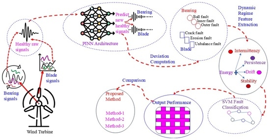
Graphical Abstract

1. Introduction

Traditional statistical models, such as ARIMA and linear regression, often fail to capture the complex temporal characteristics of wind speed time series [1]. Therefore, advanced machine learning (ML) techniques have been widely adopted to improve forecasting accuracy [2]. Various ML models, including Artificial Neural Networks (ANN), Support Vector Regression (SVR), Random Forest (RF), and XGBoost, have demonstrated better performance than conventional methods [3]. Deep learning approaches such as Long Short-Term Memory (LSTM), Convolutional Neural Networks (CNN), and Conv LSTM have further improved short-term and ultra-short-term wind speed forecasting accuracy [4]. Hybrid and ensemble forecasting models have also shown enhanced robustness and predictive capability [5].
Recent studies have applied domain adaptation techniques to enhance wind turbine condition monitoring under variable operating conditions, where conventional data-driven models often suffer from performance degradation. Liu et al. [6] employed a correlative feature–based domain adaptation approach to improve cross-domain fault diagnosis; however, its reliance on manually extracted features and domain similarity may limit scalability and generalization under highly non-stationary and complex operational environments. In addition, current studies have demonstrated significant progress in wind turbine fault diagnosis by integrating advanced signal processing techniques with deep learning and transfer learning frameworks, including compressed sensing, lightweight convolutional networks, hyper-parameter optimization, and distribution adaptation strategies. These approaches, such as compressed sensing-based CNN models, entropy-driven feature representations, and deep transfer learning architectures, have shown improved diagnostic accuracy and computational efficiency under varying operating conditions. However, their performance generally remains dependent on handcrafted feature extraction and prior domain similarity, which can restrict robustness and generalization when dealing with highly non-stationary signals and complex real-world operating environments [7,8].
Moreover, data-driven approaches, physical numerical Weather Prediction (NWP) models such as the Weather Research and Forecasting (WRF) model, combined with data assimilation techniques, have been used to improve wind speed estimation [9]. Probabilistic forecasting methods have also been introduced to quantify uncertainty and provide prediction intervals for better decision-making [10]. Despite these advances, the non-stationary and noisy nature of wind speed data remains a major challenge for accurate forecasting [11]. Signal processing techniques, especially the Wavelet Transform (WT), have been widely applied to decompose wind speed time series into multi-frequency components and reduce noise [12]. Wavelet-based preprocessing helps improve the learning capability of forecasting models by isolating meaningful patterns from raw data [13]. Attention-based causal convolutional networks improve wind speed forecasts but require large datasets and high computational resources [14]. While the multi-task LSTM model boosts short-term wind power forecasts, it still struggles when data is limited or highly variable [15]. The hybrid DSCNN-BiLSTM model can better predict wind turbine temperatures, but it still struggles when data is limited or when training becomes too complex [16]. The deep partial transfer learning network improves fault diagnosis across machines, but it can struggle when the data from different machines do not align well [17]. An intelligent observer for fault detection and data recovery in small wind turbines is developed here, but its reliability in actual turbine conditions has yet to be fully validated [18]. Ge et al. [19] used EEMD-WSST reconstruction and multi-scale entropy, but the method is computationally intensive and less suitable for real-time applications. The work of Sun et al. [20] introduced a time–frequency compression fusion method with a residual mixed-attention network for rolling bearing fault diagnosis, showing high classification accuracy, but the approach relies on a limited experimental dataset and involves considerable computational complexity that may restrict real-time industrial implementation. Li et al. [21] introduced a discriminative manifold random vector functional link neural network, which requires careful parameter tuning and may lack robustness under unseen fault conditions. Han et al. [22] combined CNN and SVM for improved classification, but interpretability and adaptability to varying sensors and operational environments are limited.
In recent studies, Zheng et al. [23] used a multi-scale CNN to detect unknown wind turbine main shaft cracks from acoustic signals, but the model was mainly tested in controlled conditions, so its real-world robustness is still uncertain. Zhang et al. [24] developed a selective state-space model to diagnose wind turbine bearing faults, but their results are based on limited test data, so their effectiveness under real-world operating conditions still needs further validation. Li et al. [25] developed a system combining knowledge graphs and large language models to support wind turbine fault maintenance, but it has only been tested in simulations, so its performance in real-world operations is still uncertain. Nevertheless, existing Wavelet–SVR models still face challenges related to optimal wavelet selection, decomposition level determination, and SVR parameter tuning across different wind regimes and geographical locations [26]. An adaptive federated framework was developed to detect faults in wind turbines, showing promising accuracy across multiple datasets, but the study was only tested on a few turbines, which may limit its applicability to larger wind farms [27]. Therefore, further research is needed to improve the adaptability and forecasting accuracy of Wavelet–SVR-based wind speed prediction models [28]. Current studies on bearing and blade fault diagnosis have achieved high accuracy using deep learning and machine learning techniques. Grover and Turk [29] applied transfer learning on bispectrum contour maps, but their model may not generalize well under varying operational conditions. Zaniboni et al. [30] used learning-based methods for wind turbine blade monitoring, yet their approach relies on static thresholds and limited sensor types, reducing sensitivity to subtle faults. Sharma et al. [31] combined higher-order spectral analysis with machine learning, showing good results in controlled settings but with limited robustness to noise and operational variations. Yoo et al. [32] developed a lightweight deep learning model for the CWRU dataset, which performs well on benchmark data but lacks validation under real industrial conditions. The feasibility of using small wind turbines in urban areas as a renewable energy source, highlights both their energy potential and the practical challenges associated with turbulent and built-up wind conditions [33]. Fadaei et al. [34] focused on offshore wind energy, which has gained significant attention due to its high energy potential. Araveti et al. [35] examined wind energy potential for renewable energy communities by comparing different wind data sources to improve the accuracy of wind resource assessment and support better planning decisions. Collectively, these studies reveal gaps in generalization, robustness, and interpretability. The present work addresses these limitations by integrating a PINN with deviation-based dynamic regime features, improving fault detection under practical operating conditions. The novelty of the study is as follows:
  • PINN learns a healthy reference model that embeds system physics into neural network training, not just learning from data.
  • Deviation-based dynamic regime features extraction to highlight fault-relevant information, handle non-stationarity, reduce noise effects, and create robust features for machine learning classifiers.
  • Faults detected by PINN deviation-interpretable SVM multi-class classification under small data dynamic condition, which demonstrates how the PINN is embedded into the fault-diagnosis pipeline.
  • Energy-based other regime feature combinations are observed, which capture not only how strong the fault is but also how it evolves, resulting in a more reliable and meaningful fault diagnosis.
The next sections of this paper are organized as follows. Section 2, proposal of the overall algorithm, describes the introduction to deviation-based dynamic regime features, PINN-based healthy reference framework, and the overall algorithm. In Section 3, experimental design of the proposed method with experimental parameters, equipment, and procedure in detail, and a brief workflow discussion of the comparison of three different methods. Result discussions of the proposed method on both datasets and comparisons are given in Section 4. Section 5 provides the conclusion with limitations and future work.

2. Proposal of the Overall Algorithm

2.1. Introduction to Deviation-Based Dynamic Regime Features

Deviation is a measure of how much a system’s behavior departs from a reference healthy state. In fault diagnosis, it quantifies changes in operational patterns by comparing the current signal to a baseline (healthy) signal. Consider a vibration signal x(t) measured from a component (bearing, blade), and xref(t) be the reference healthy signal. The deviation signal d(t) is defined as shown in Equation (1). In practice, deviation emphasizes small changes that may not be obvious in raw signals, making it useful for early fault detection.
d ( t ) = x ( t ) x r e f ( t )
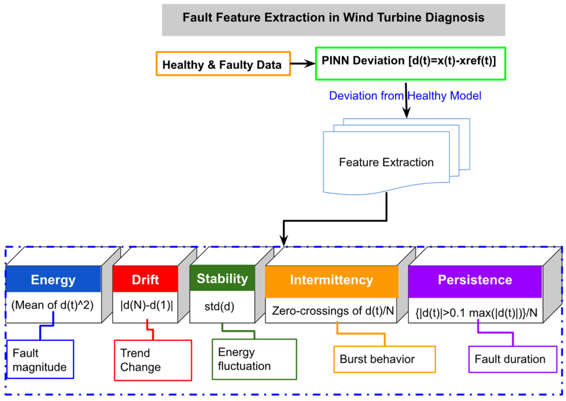
Dynamic regime features, including energy, drift, intermittency, persistence, and stability, describe how a system evolves, particularly in systems that are non-stationary or have time-varying dynamics, as shown in Figure 1. They are used to capture the temporal patterns, transitions, and variations in the system, beyond just static averages or single-time statistics. Common in wind turbines, bearings, motors, or power systems, where signals change depending on operational conditions.
Energy measures the signal strength in a time segment, which can indicate faults and high energy in deviation indicates stronger fault manifestation as shown in Equation (2). Drift captures slow trends or shifts over time in the signal baseline and shows long-term changes in operating regime which are estimated by fitting a linear trend to d(t) as shown in Equation (3). Intermittency measures the occurrence of bursts or irregular events in the system which is important in detecting transient faults as shown in Equation (4). Persistence indicates how long a certain regime or pattern continues; high persistence means the system remains in a state for a long time as shown in Equation (5). Stability measures resilience or variability of the regime, unstable regimes fluctuate a lot, while stable regimes are consistent over time as shown in Equation (6).
E n e r g y = 1 N i = 1 N d i 2  
D r i f t = d ( t ) | d ( t N ) d ( t 1 ) |
I n t e r m i t t e n c y = 1 N 1 i = 1 N 1 indicator function ( I ) ( | s i g n ( d i + 1 ) s i g n ( d i ) | > 1 )
P e r s i s t e n c e = N u m b e r   o f   s a m p l e s   w i t h | d i | > t h r e s h o l d N
S t a b i l i t y = var ( d ) = S t d ( d ) = 1 N i ˙ = 1 N ( d ( i ) d ¯ ) 2
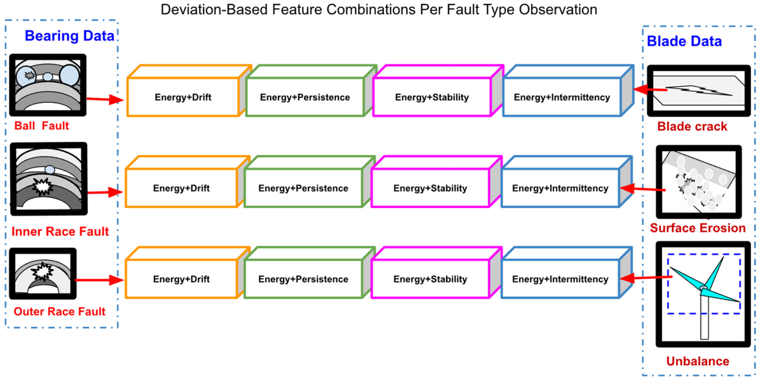
The fault classification performance improves when multiple deviation-based regime features are combined, as each feature captures a different physical characteristic of the blade and bearing fault. By observing, it is possible to understand which features contribute most to distinguishing faults. This analysis helps identify the complementary information provided by each feature pair, showing how certain combinations capture both the magnitude and temporal characteristics of faults. These insights guided the selection of the most effective features for classification and highlighted the benefits of feature fusion in improving performance, as shown in Figure 2.

2.2. Introduction to PINN-Based Healthy Reference Framework

In complex rotating systems such as wind turbines, the vibration of components, like blades and bearings, follows predictable physical laws under healthy operating conditions. To monitor structural integrity, it is important to have a model that represents these normal dynamics accurately. PINN provides a way to construct such models by combining the representational flexibility of neural networks with knowledge of the underlying physics.
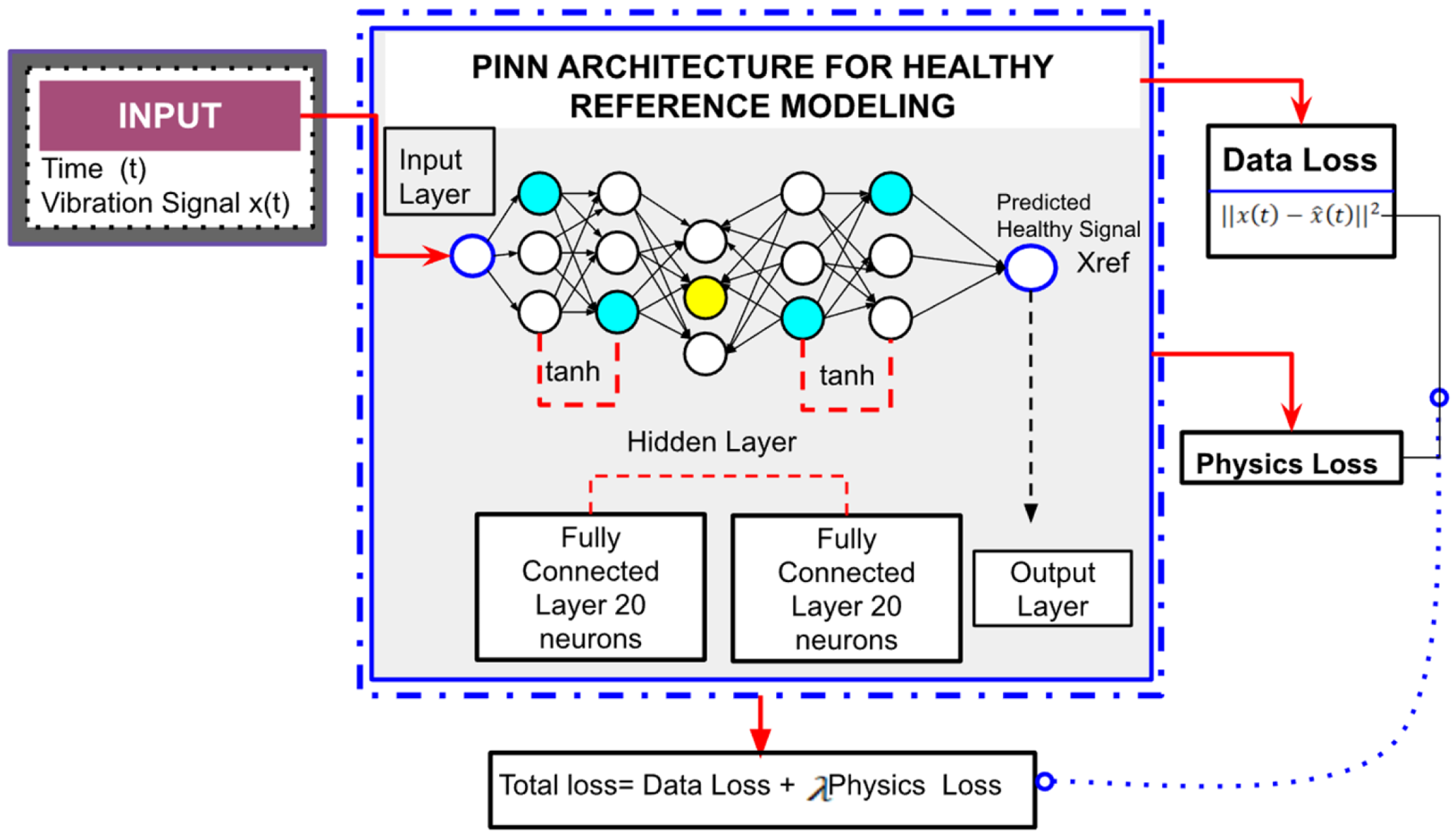
In this framework, the network is designed to capture the expected smooth evolution of healthy vibrations while respecting physical constraints, such as continuity and gradual changes over time. By doing so, the network establishes a reference model of normal system behavior without explicitly relying on fault-labeled data, as shown in Figure 3. This approach allows deviations in measured signals to be interpreted as faults.
PINN offers several theoretical advantages for this application. First, it incorporates prior knowledge of the system, which improves generalization and reduces sensitivity to noise. Second, it enforces smoothness and consistency in the modeled response, which is critical for detecting subtle faults in blades and bearings. Third, differentiable activation functions, such as hyperbolic tangent, allow the network to represent continuous physical processes and compute temporal derivatives when needed. Accordingly, the measured vibration signal is expressed as shown in Equations (7) and (8). The network approximates the healthy response as shown in Equation (9). The PINN is trained by minimizing a physics-informed loss function as shown in Equations (10)–(12). Overall, the theoretical strength of PINN lies in its ability to create a physically consistent baseline for healthy components. This baseline forms the foundation for detecting deviations caused by faults, providing a reliable and interpretable approach to condition monitoring in wind turbines.
x ( t ) = x h ( t ) + ε ( t )
x f ( t ) = x h ( t ) + d ( t )
h ( l ) = tanh ( W ( l ) h ( l 1 ) + b ( l ) )
L ( θ ) = L d a t a + λ L p h y S
L d a t a = 1 N i = 1 N ( x ^ h ( t i , θ ) x ( t i ) 2 ) = 1 N i = 1 N ( x i x ^ i ) 2 = x ( t ) x ^ ( t ) 2
L p h y s =     1 N 2 i = 2 N 1 ( x ^ i + 1 2 x ^ i + x ^ i ˙ 1 Δ t 2 + ω 2 x ^ i ) 2 = d 2 x ^ ( t ) d t 2 + ω 2 x ^ ( t ) 2
In this study of PINN, lambda is used for controlling the importance of the physics-based constraint relative to data fitting. A small value ensures that the network primarily learns an accurate, healthy reference signal, while the physics term acts only as a soft regularizer to keep the prediction smooth and physically reasonable, and the purpose of lambda ω in this work is regularization and reference modeling, not physical frequency estimation.

2.3. Introduction to the Overall Algorithm

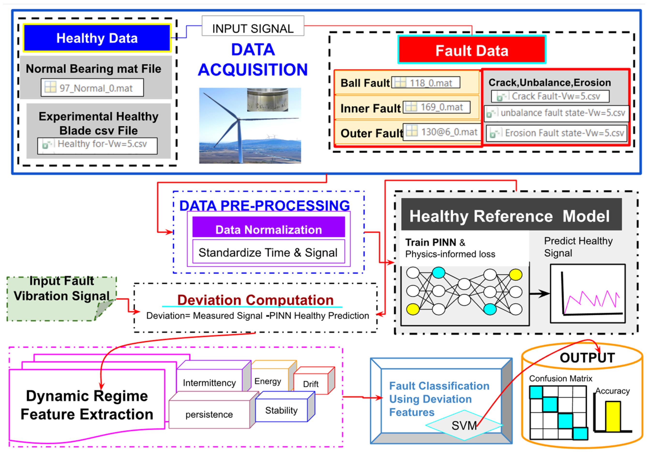
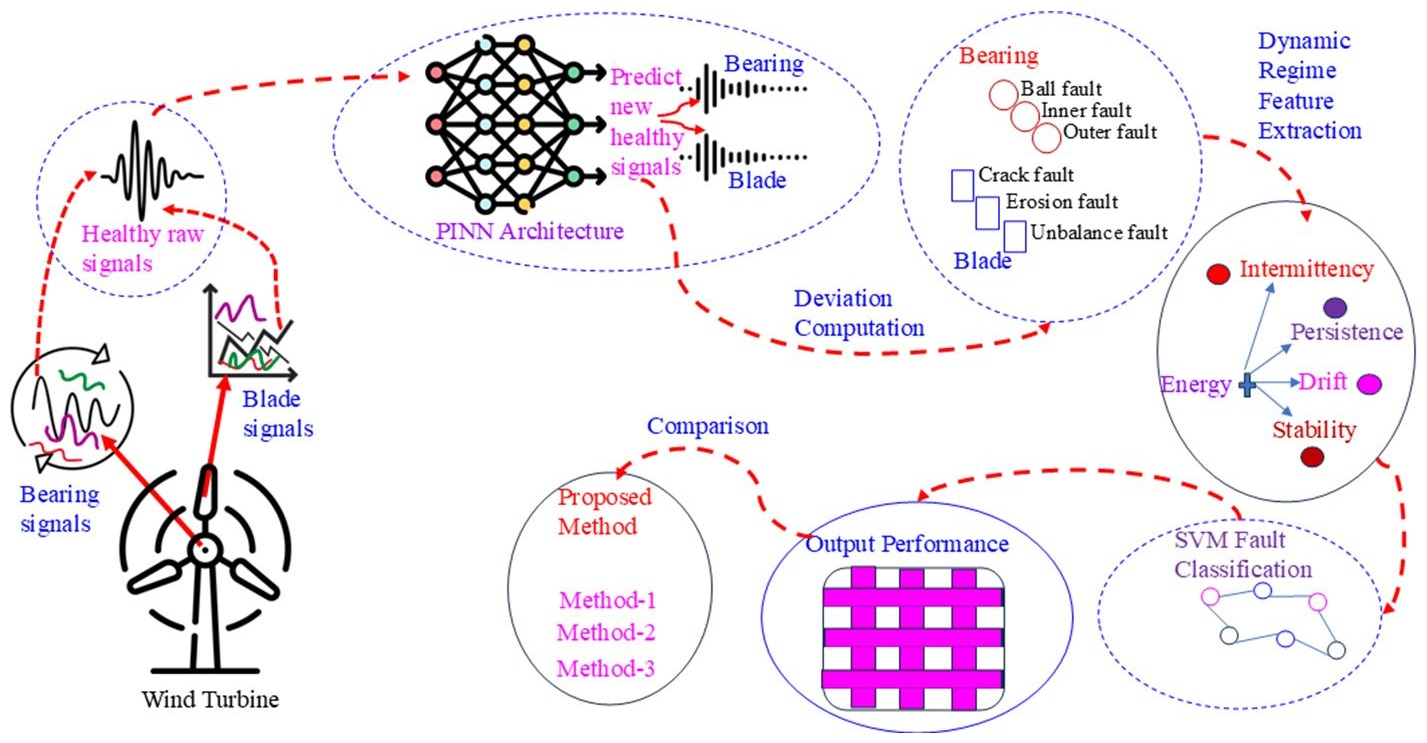
PINN and dynamic regime feature-based fault diagnosis is the main algorithm in this work, as shown in Figure 4.
Step 1: Data Acquisition and Healthy Data Preparation
Collected vibration signals from healthy blades and bearings under normal operating conditions. Next, removed invalid, noisy measurements. Lastly, normalized the data to standardize amplitude and scale.
Step 2: Healthy Reference Modeling with PINN
Defined a neural network with fully connected layers and hyperbolic tangent activations. Then trained the network using healthy signals, incorporating a physics-informed constraint that enforces smoothness, and optimized the network to accurately represent the expected dynamics of healthy blades and bearings.
Step 3: Fault Signal Analysis
After creating a healthy reference model, collected vibration signals under faulty conditions. Fault signals were normalized by using healthy data statistics. The trained PINN was used to predict the healthy baseline for each measurement. Deviation signals were computed by subtracting the predicted healthy response from the measured signal.
Step 4: Feature Extraction
Dynamic regime features were extracted from deviation signals and organized into vectors for classification.
Step 5: Fault Classification
Trained an interpretable classifier, support vector machine, using labeled feature vectors and applied the classifier to identify the fault type for each new measurement, distinguishing between:
Blade faults: cracks, erosion, unbalance;
Bearing faults: ball, inner race, outer race defects.
Step 6: Performance Evaluation
Evaluated the classification accuracy and analyzed confusion matrices to verify robustness across varying operational conditions and component types.

3. Experimental Design and Analysis

This section represents the experimental parameters, equipment, and process in detail of the proposed method for both datasets, and a brief workflow explanation of three different comparison methods.

3.1. Acquisition of Data 1

3.1.1. Experimental Equipment

The rolling bearing dataset is obtained from the Case Western Reserve University (CWRU) bearing data center [36]. It includes three fault types in a healthy condition. All data are collected from the drive end at a sampling rate, which is analyzed offline using software as shown in Table 1.

3.1.2. Experimental Parameters

The detail parameters of the CWRU-bearing dataset are shown in Table 2.

3.1.3. Experimental Procedure

Vibration signals from drive-end accelerometers of bearings are collected from the CWRU dataset, including healthy bearings and bearings with ball, inner race, and outer race faults. A segment of the healthy vibration signal is first selected, then healthy bearing signals are used to establish a reference by centering the data and smoothing the normalized response, capturing the typical vibration pattern under normal operation. The six-layer physics-informed neural network is designed to learn the normal dynamic behavior of the bearing vibration signal. The input layer receives the normalized (t) time variable, which represents the temporal progression of the vibration signal. This time input allows the network to model how the vibration evolves rather than treating samples as independent points. The signal (z) then passes through the first fully connected hidden layer with 20 neurons, where weighted (ω) combinations of the time input are formed as shown in Equation (13). This layer begins to capture basic temporal patterns in the healthy vibration response.
z 1 ( j ) = ω 1 ( j ) t + b 1 ( j ) , j = 1,2 , , 20
A nonlinear activation function is applied to allow the network to represent complex, nonlinear dynamics that cannot be described by simple linear models. Each neuron learns a different transformation of time as shown in Equation (14).
a 1 ( j ) = tanh ( z 1 ( j ) )
The second fully connected hidden layer, also containing 20 neurons, further refines these representations. By stacking two hidden layers, the network gains sufficient depth to model smooth yet complex vibration behavior, such as periodicity and gradual changes associated with normal bearing operation. Each neuron in the second hidden layer receives all outputs from layer one, as shown in Equation (15).
a 2 ( k ) = tanh ( j = 1 20 ω 2 ( k , j ) a 1 ( j ) + b 2 ( k ) ) , k = 1,2 , , 20
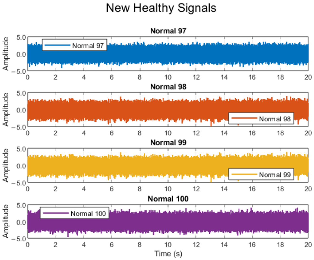
Finally, the output layer produces a single continuous value corresponding to the estimated healthy vibration response at each time instant. Rather than predicting fault conditions, the network focuses solely on reproducing the normal vibration pattern. Whenever a test time series is input, the PINN estimates a new healthy signal and provides a reference used to compute deviation for fault detection, as shown in Figure 5 and Equation (16).
x ^ ( t ) = d ^ ( t n ) = k = 1 20 ω 3 ( k ) a 2 ( k ) + b 3
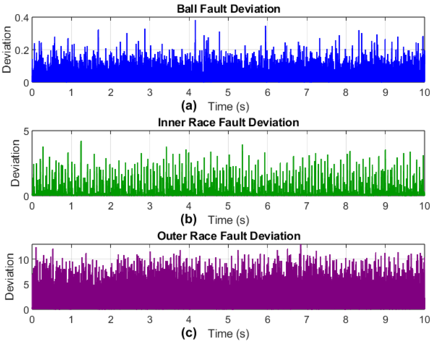
In Figure 6 and Equation (17).
D e v i a t i o n = d ( t ) = x f ( t ) x ^ ( t ) ,   F a u l t   v s .   H e a l t h y
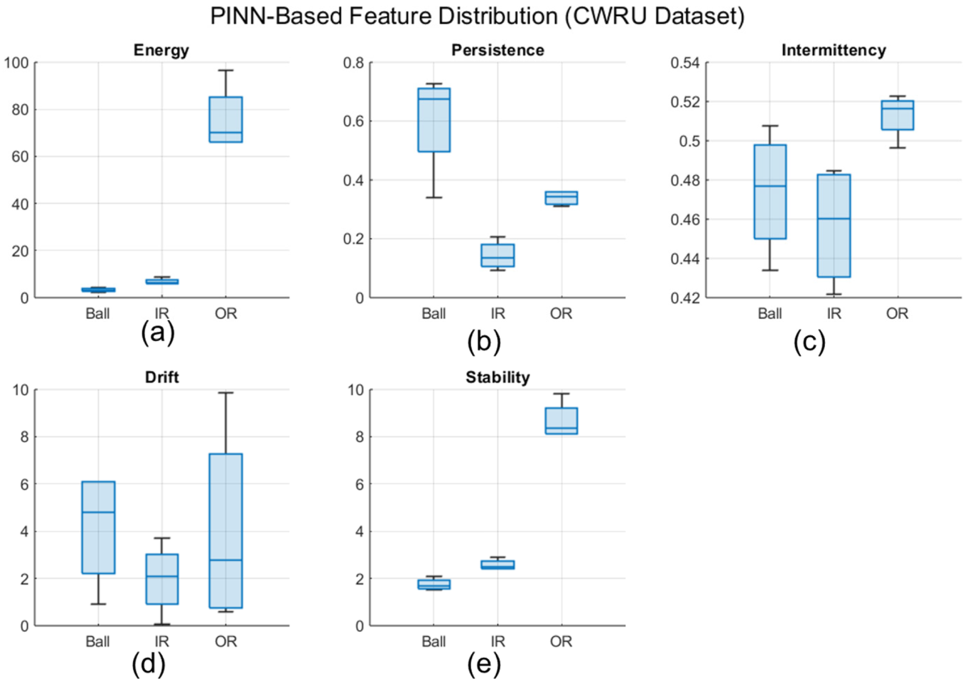
From these PINN deviations, features are extracted and distributed to characterize fault behavior, including energy (representing fault magnitude), temporal persistence, intermittency, drift, and stability (behavior) as shown in Figure 7.
For each fault file, a single set of feature values is obtained, which represents the fault behavior and is used for SVM-based classification, as shown in Table 3. The training of the neural network for healthy signal modeling is monitored via the loss over epochs, as shown in Table 4.
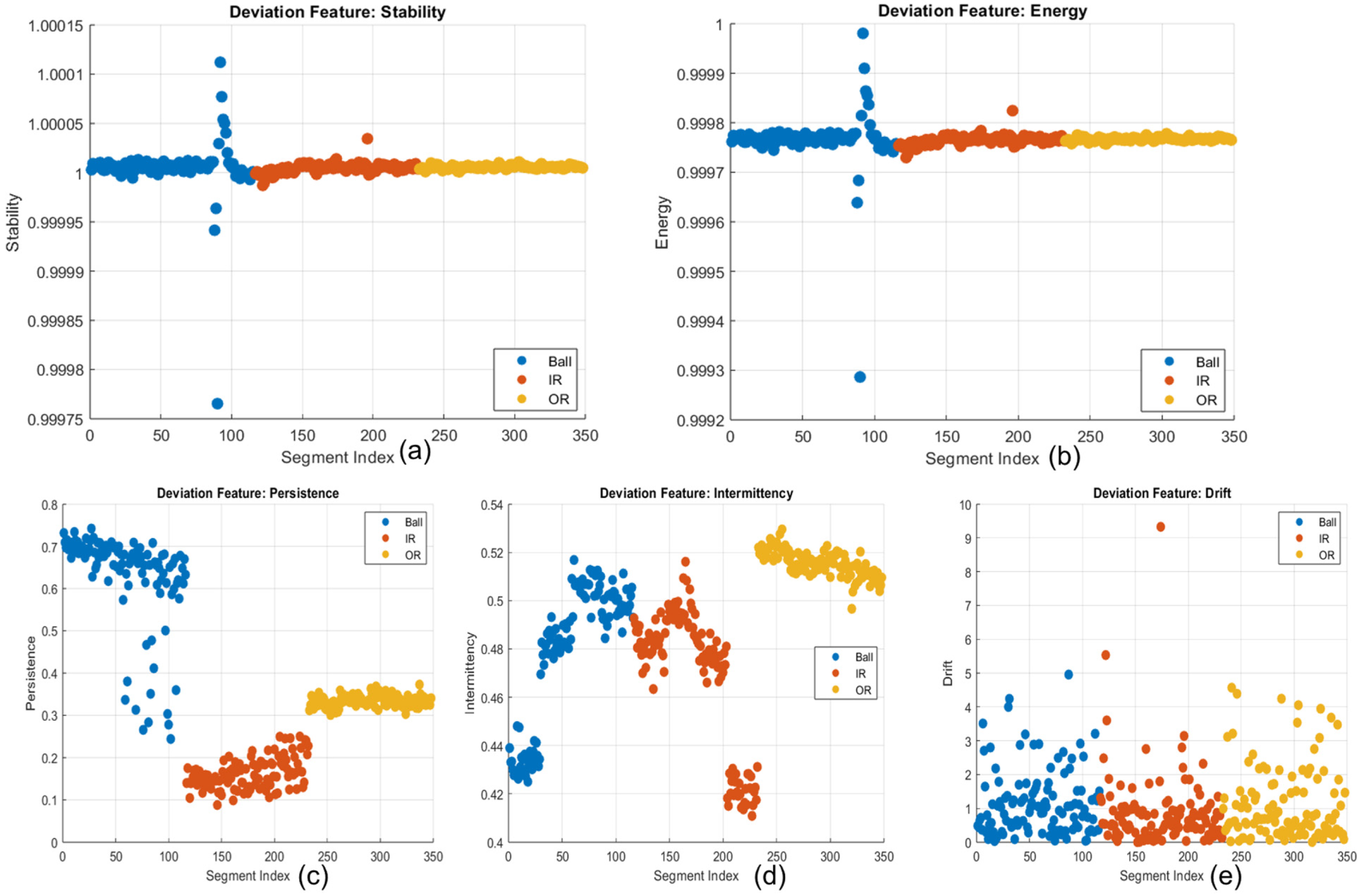
In addition, the experimental task is examined in combinations of features, including energy with persistence, energy with intermittency, energy with drift, energy with stability, and all features together, which reveal which features most effectively represent fault behavior and demonstrate how integrating complementary information can enhance SVM classification performance. A total of 350 segment samples of each dynamic regime feature is used for testing fault classification, as shown in Figure 8. The fault classification is performed primarily using the energy feature, where thresholds based on percentiles of the energy distribution distinguished between ball, inner race, and outer race faults. The performance of the method was evaluated using a confusion matrix and overall classification accuracy, precision, recall, and F1 score, as shown in Equations (18)–(21).
A c c u r a c y = N u m b e r   o f   c o r r e c t   p r e d i c t i o n s T o t a l   p r e d i c t i o n s × 100 %
P r e c i s i o n = T P T P + F P h e r e , T P = T r u e   p o s i t i v e , F P = F a l s e   P o s i t i v e
R e c a l l = T P T P + F N h e r e , F N = F a l s e   N e g a t i v e
F 1 = 2 × P r e c i s i o n × R e c a l l P r e c i s i o n + R e c a l l

3.2. Acquisition of Data 2

3.2.1. Experimental Equipment

The experimental blade dataset is collected, which consists of 35 files in the form of CSV [37]. Table 5 shows the equipment of the blade dataset.

3.2.2. Experimental Parameters

In this study, 28 files are used. Each file contains two columns. The first column represents the time in seconds on the X-axis, while the second column represents amplitude on the Y-axis. In 28 files include three types of faults of the blade in a healthy condition. The dataset comprises single-axis vibration measurements acquired from a wind turbine subjected to variable load conditions resulting from changes in wind speed range from 1.3 to 5.4 m/s, as shown in Table 6.

3.2.3. Experimental Procedure

The study aimed to detect faults in wind turbine blades using deviation-based measurements. At first, blade vibrations are collected under varying wind speeds, capturing both healthy blades and blades with specific faults such as unbalance, erosion, and cracks, which are loaded using MATLAB. These measurements provide the foundation for analyzing how different fault types affect blade vibrations. The healthy blade data are first compiled and carefully cleaned to remove any invalid values. Normalized time (t) and vibration amplitude (x) using the mean and standard deviation of the healthy dataset, as shown in Equation (22).
t n o r m = t t ¯ S t   d ( t ) ; x n o r m = x x ¯ S t   d ( x )  
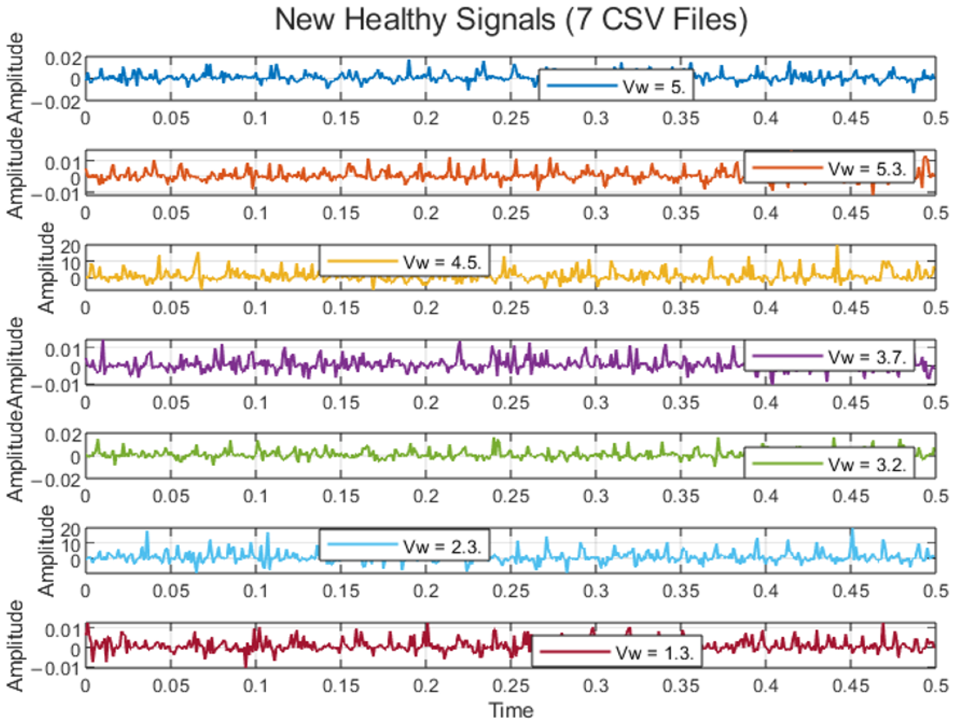
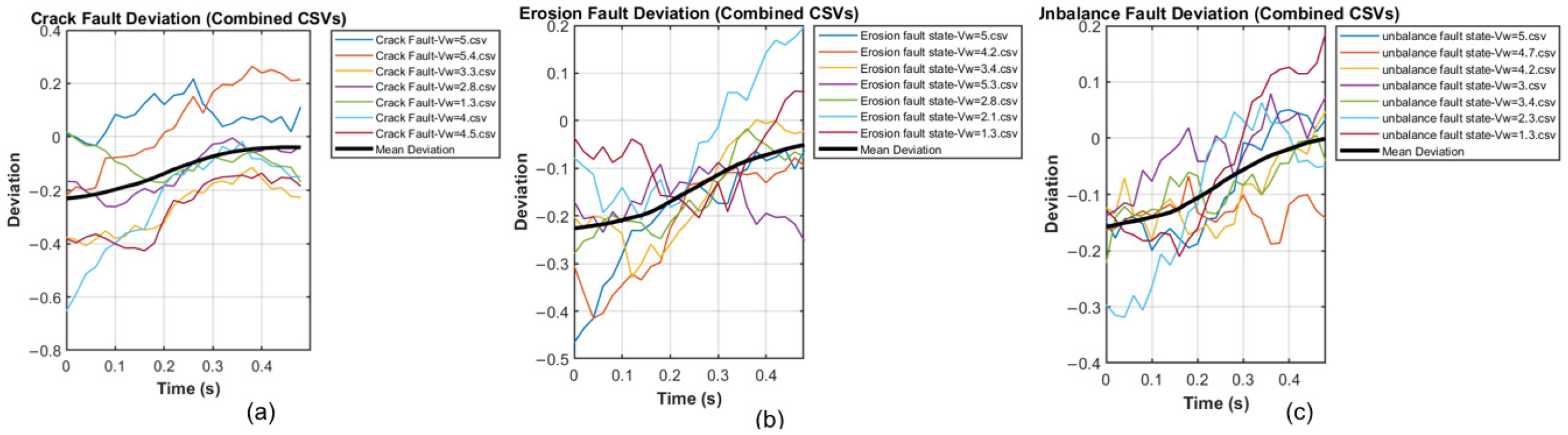
These healthy measurements are used to estimate a reference signal, as shown in Figure 9, representing healthy blade behavior. By comparing the faulty blade vibrations to this reference, deviations caused by faults are identified as shown in Equation (23) and Figure 10.
d ( t ) = x f a u l t , n o r m ( t ) x P I N N ( t )
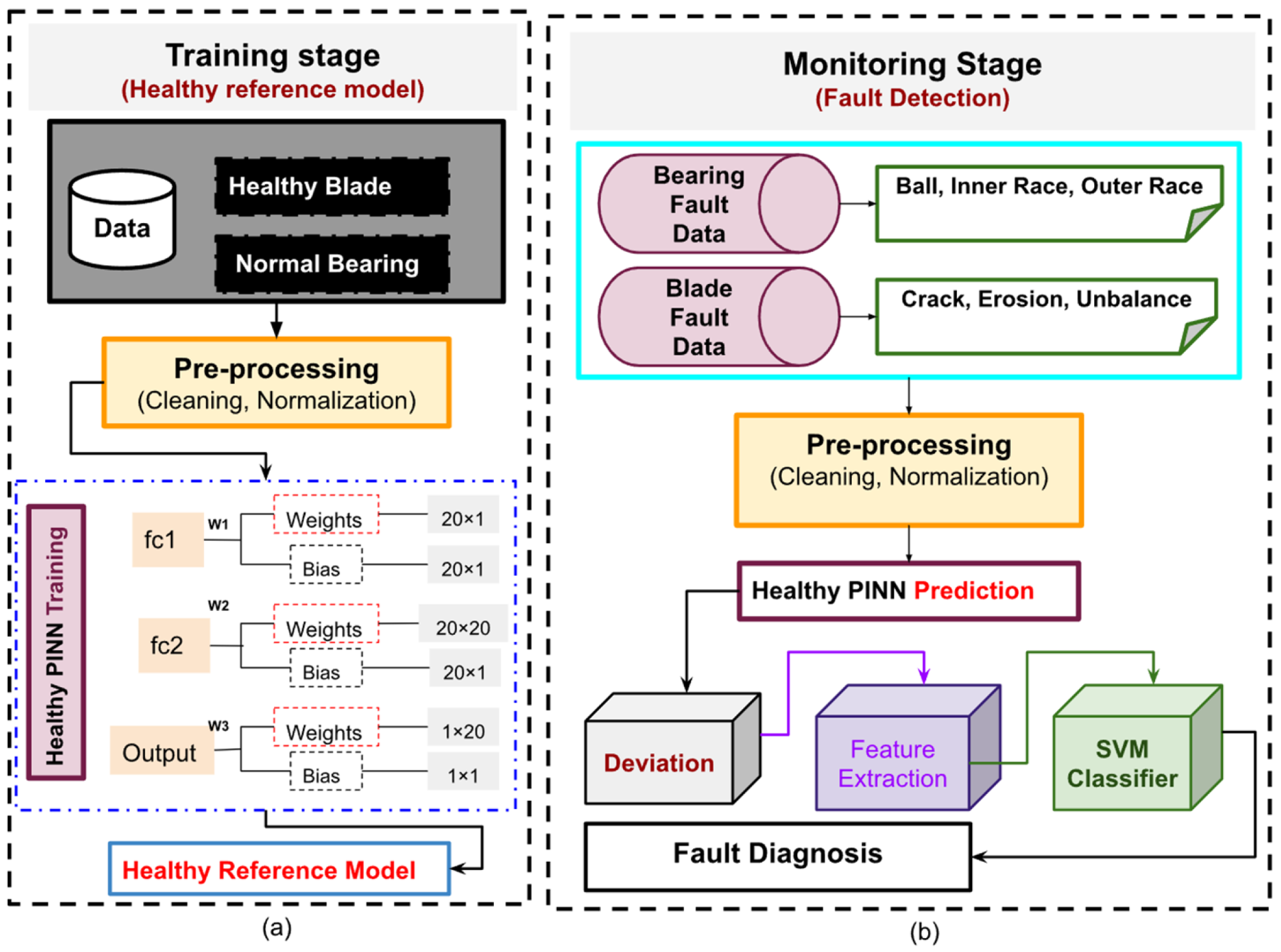
For the blade data process, the training and monitoring stages are the same as the bearing data procedure. During the training stage, only healthy vibration data are used to teach the PINN the normal dynamic behavior of the blade at different wind speeds, and the model learns to reproduce the healthy response while respecting the physical constraint embedded in the loss function. This trained network serves as the baseline reference model. The training process with parameter values for each speed is shown in Table 7.
In the monitoring stage, new incoming signals are compared with the healthy response predicted by the trained PINN. Next, the deviation between the two signals is analyzed, and dynamic regime features are extracted from this deviation. After extraction, these features are then fed into the SVM to identify the type of fault, as shown in Figure 11.
Energy, calculated from the deviation signal, served as the primary indicator of fault magnitude. Additional features captured temporal behavior, including trends over time, irregular bursts, sustained deviations, and fluctuations in signal stability. These features together provided a comprehensive characterization of the faults, though energy alone carried the most significant information about fault severity. Each fault file is summarized into a single feature vector that captures its dynamic characteristics and serves as the input for interpretable classification, as shown in Table 8.
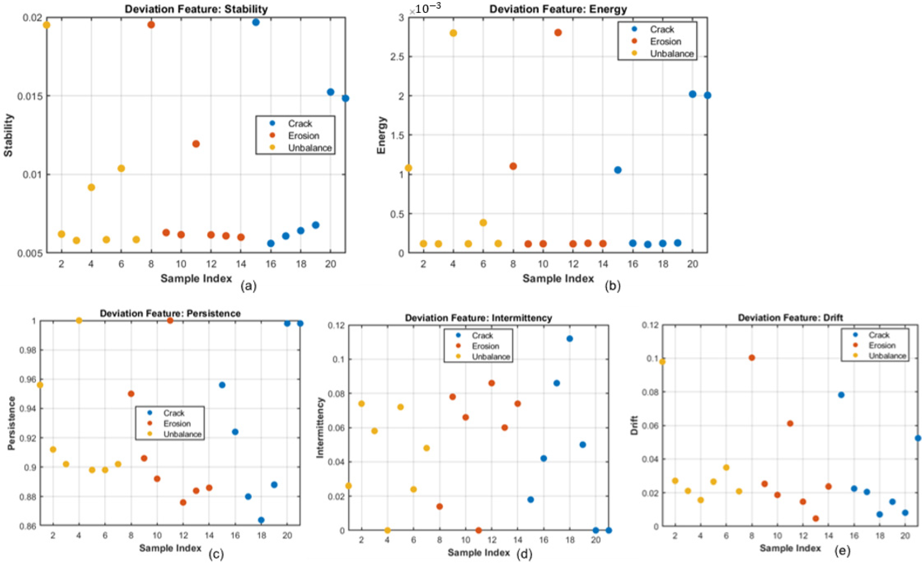
A total of 21 fault test samples, including crack, erosion, and unbalance cases under varying wind speeds, are used for validation as shown in Figure 12. The model’s performance is evaluated by calculating its accuracy, precision, recall, F1 score, and examining the confusion between classes, allowing assessment of which faults are most easily identified and which are more challenging.

3.3. Comparison of Three Different Methods Pipeline

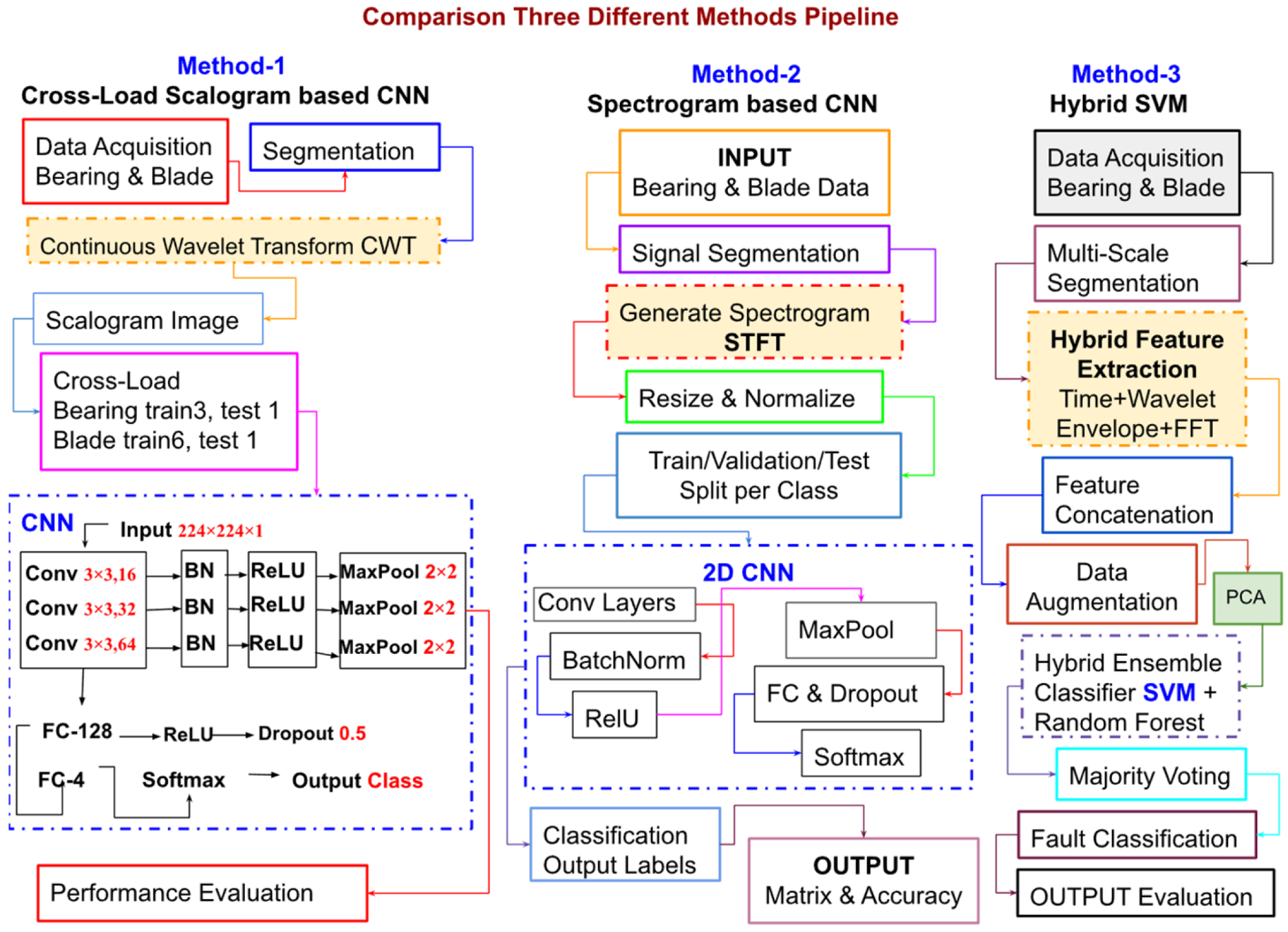
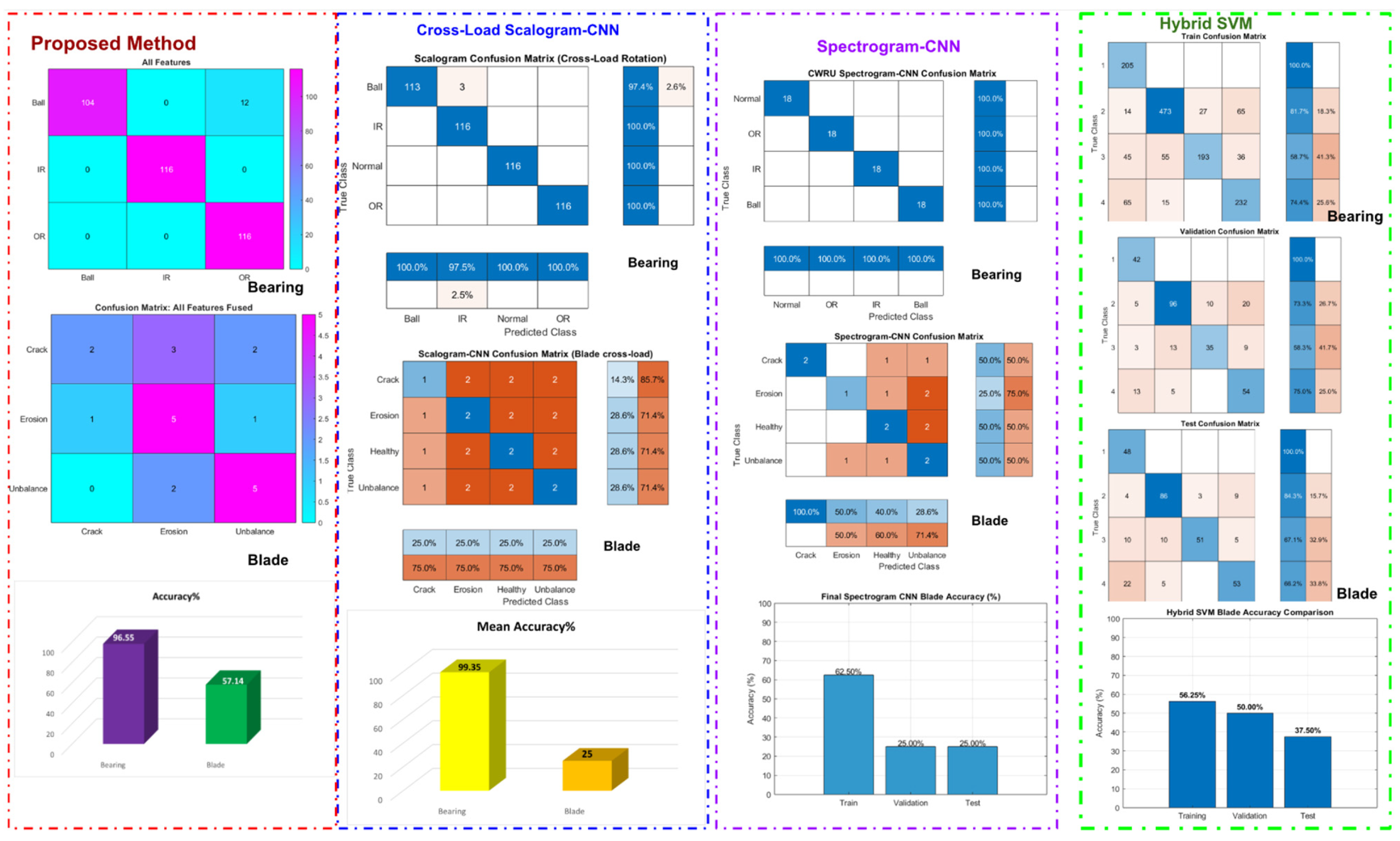
To evaluate the performance of the proposed approach, three different methods are considered for comparison: Cross-Load Scalogram–CNN, Spectrogram–Convolutional Neural Network (CNN), and a Hybrid SVM-based model. The Cross-Load Scalogram–CNN converts vibration signals into time–frequency scalogram images using continuous wavelet transform and tests the model’s ability to generalize across different wind speeds, blade, and bearing faults. The Spectrogram–CNN follows a similar deep learning framework but uses the short-time Fourier transform to generate spectrogram images for the classification of both types of data. In contrast, the Hybrid SVM method is based on manually extracted statistical features from time, frequency, wavelet, and envelope domains, followed by dimensionality reduction and ensemble classification. While the CNN-based approaches automatically learn relevant features from image representations, the Hybrid SVM relies on carefully designed features. This comparison provides a balanced evaluation between traditional feature engineering and deep learning techniques for wind turbine blade and bearing fault diagnosis, as shown in Figure 13.
Table 9, Table 10 and Table 11 show three comparison method parameters and results of both datasets.

4. Result and Discussion

This section represents all experimental results, analyses, and comparisons on both datasets.

4.1. Bearing Dataset Result and Discussion

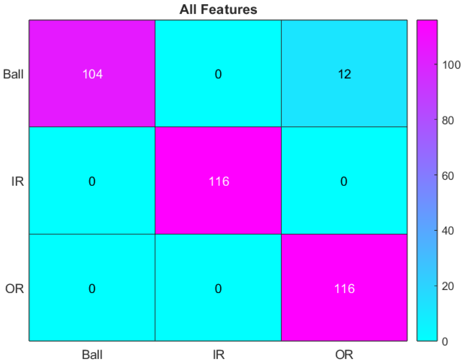
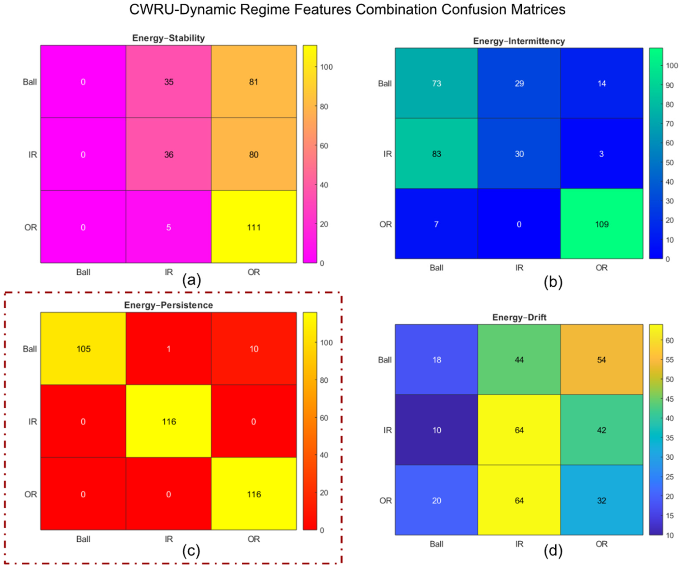
Confusion matrices summarize the performance of a classification model by comparing the predicted labels with the actual labels. It helps to understand not just overall accuracy but also the types of errors the model makes. The combination of all features confusion matrix shows that the classifier correctly identified 104 ball faults, 116 inner race and outer race faults, while 12 ball samples are misclassified as outer race as shown in Figure 14. The classification accuracy obtained using the energy with persistence feature pair is comparable to that achieved using all fused features; in this combination 1 and 10 ball samples are misclassified as inner race and outer race. This indicates that Energy and Persistence together capture the dominant fault characteristics; namely, fault severity and duration. The remaining feature combinations provide complementary but less discriminative information, and therefore do not significantly improve performance beyond what is already achieved by this compact feature set, as shown in Figure 15.
Total test samples of all feature combination = 104 + 0 + 12 + 0 + 116 + 0 + 0 + 0 + 116 = 348
Correct predictions = 104 + 116 + 116 = 336
Accuracy = 336/348 = 0.96551724 = 96.55%
Total test samples of combination feature Energy with Persistence = 105 + 1 + 10 + 0 + 116 + 0 + 0 + 0 = 116 = 348
Correct prediction = 105 + 116 + 116 = 337
Accuracy = 337/348 = 0.9683 = 96.83%
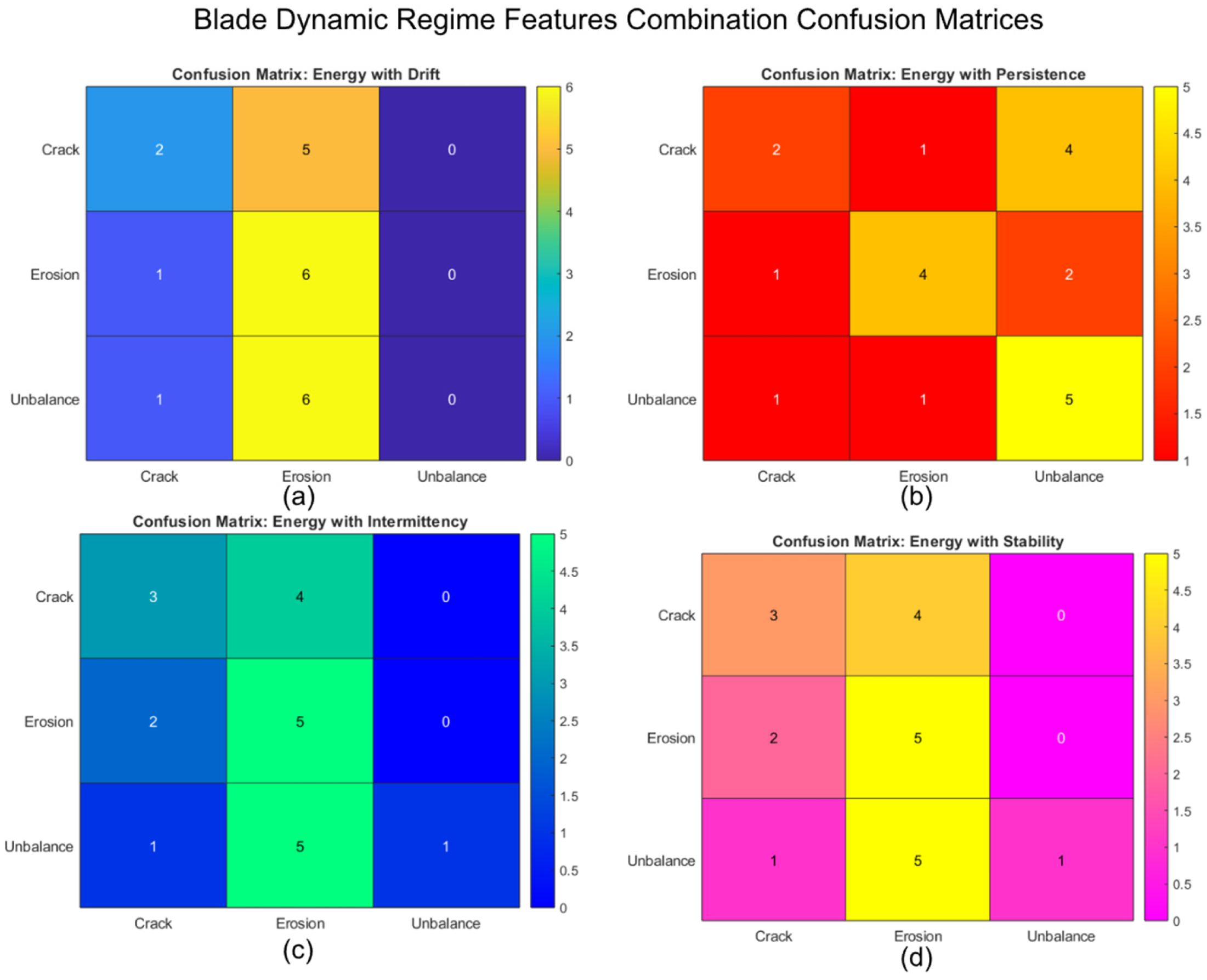
According to the calculation combination feature of Energy with Drift Accuracy = 114/348 = 0.3276 = 32.76%
Energy with Stability Accuracy = 147/348 = 0.4224 = 42.24%;
Energy with Intermittency Accuracy = 212/348 = 0.6091 = 60.91%
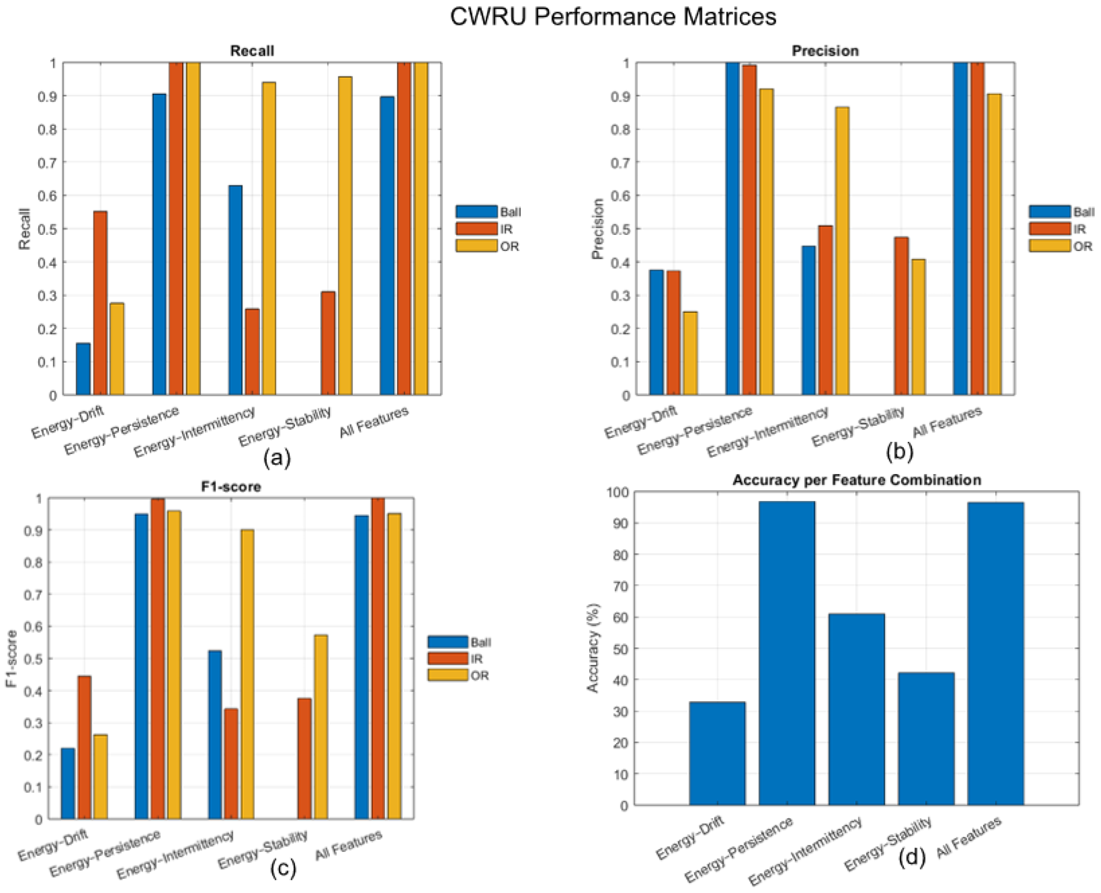
For the inner race fault class, the proposed method using the combined Energy with Persistence and all features fused achieved perfect classification performance, obtaining a recall, precision, and F1-score of 1.00. This indicates that all inner race samples are correctly identified with no false positives or false negatives, while outer race fault class and ball fault class achieved only a recall and precision of 1.00, as shown in Figure 16.

4.2. Blade Dataset Result and Discussion

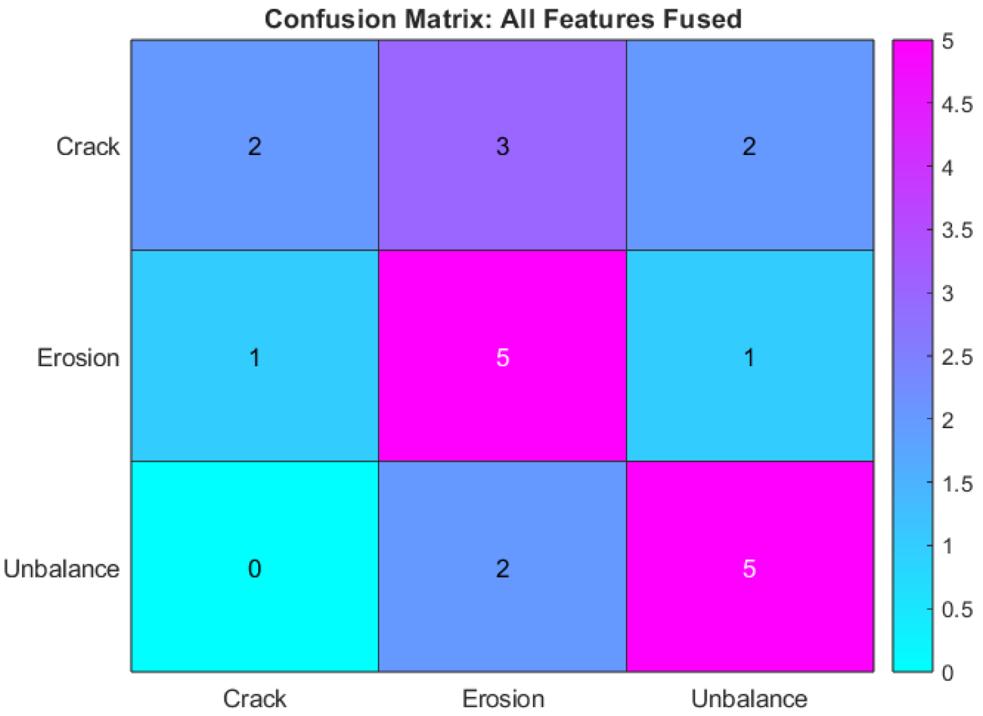
For blade fault classification, the highest accuracy is achieved when all deviation-based dynamic regime features are fused. This indicates that blade faults exhibit complex vibration behavior involving simultaneous changes in magnitude, duration, intermittency, drift, and variability. Unlike simpler feature combinations, the fused feature set captures these interacting characteristics more effectively, leading to improved class separability and higher classification accuracy, as shown in Figure 17 and Figure 18.
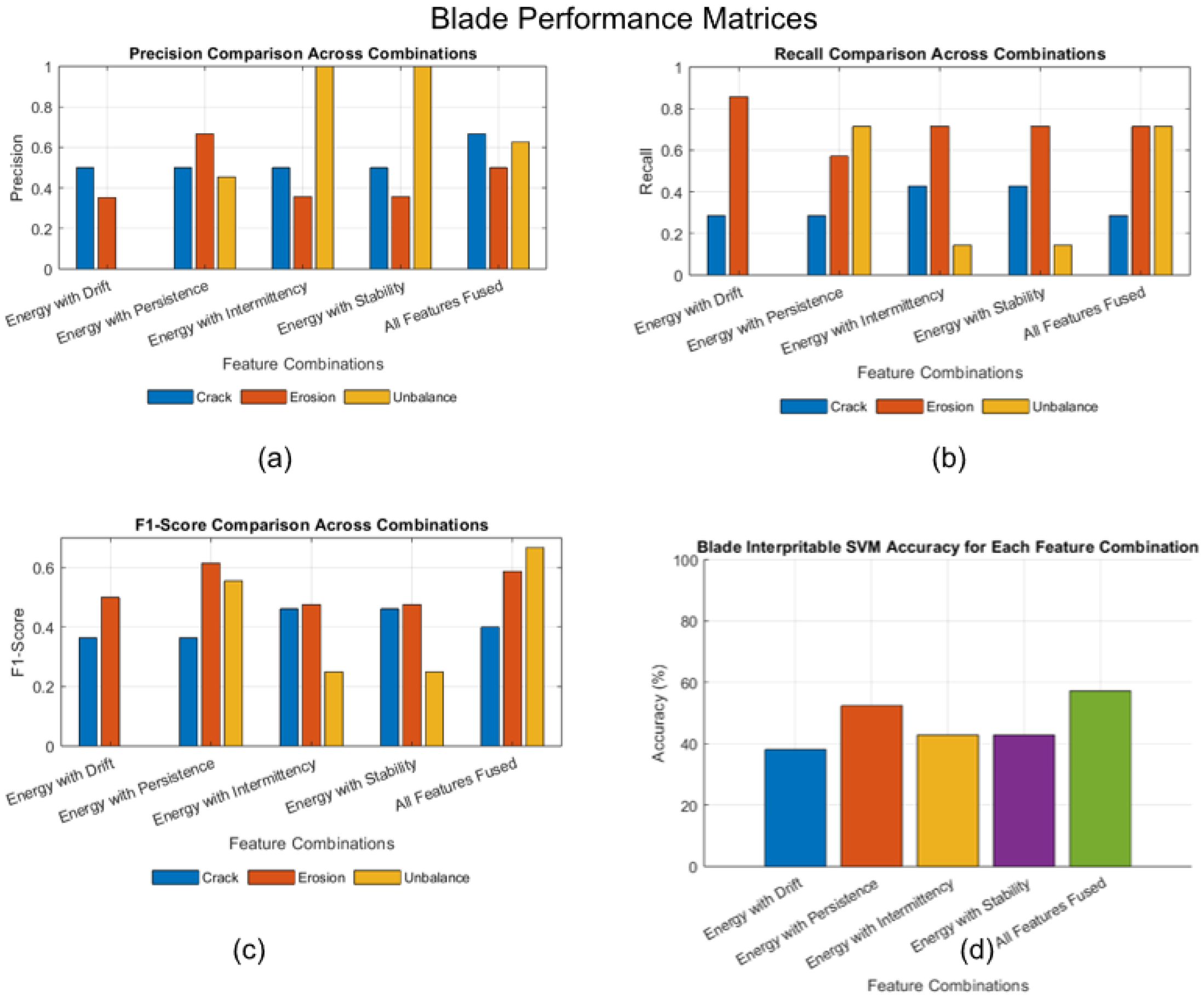
The performance matrices results show that different faults respond better to different feature combinations, as shown in Figure 19. Table 12 shows the highest performance classification of each fault based on features.
Total blade test samples of combination all features = 2 + 3 + 2 + 1 + 5 + 1 + 0 + 2 + 5 = 21
Correct predicted = 2 + 5 + 5 = 12
Accuracy = 12/21 = 0.571428 = 57.14%
According to the calculation, the accuracy of Energy with Persistence = 11/21 = 0.5238 = 52.38%
Energy with Stability Accuracy = 9/21 = 0.4285 = 42.85%
Energy with Drift Accuracy = 8/21 = 0.3809 = 38.09%
Energy with Intermittency Accuracy = 0.4285 = 42.85%

4.3. Comparison with Three Different Methods

Figure 20 shows the classification accuracy comparison between the proposed method and three existing approaches on the bearing and blade datasets. Method-1 cross-load scalogram–CNN and Method-2 spectrogram–CNN achieve high accuracy on the bearing dataset, 99.35% and 100%. However, both methods exhibit substantial performance degradation on the blade dataset, achieving only 25% accuracy. This indicates limited generalization capability across different mechanical components. Method-3 hybrid-SVM shows relatively balanced but lower performance on both datasets, 77.78% on bearing and 37.50% on blade. In contrast, the proposed method exhibits stable and reliable performance across both datasets, confirming its stronger feature generalization capability. The proposed method achieves 96.55% accuracy on the bearing dataset and 57.14% accuracy on the blade dataset. Overall, the proposed method provides better accuracy and robustness, making it more suitable for practical industrial applications where operating conditions and component types vary.

5. Conclusions

This work presented a fault diagnosis framework based on dynamic-regime feature extraction using a PINN trained with healthy signals. The PINN model, normal system dynamics, and faults are identified from deviations between predicted and measured responses. Extracted dynamic regime features are then classified using an interpretable SVM and observed energy-based combination for each type of fault detection on bearing and blade datasets. Experimental observation reveals that energy with a persistence feature combination is more robust than other regime combinations for both datasets. Additionally, the evaluation of fused dynamic regime features achieved 96.55% accuracy on the bearing dataset and 57.14% on the blade dataset. The method achieves high accuracy for bearings but performs less effectively for turbine blades, indicating both a limitation and a direction for future research. To overcome this limitation, future work may focus on improving the representation of turbine blade data and refining feature extraction methods. In this paper, the practical application direction is rotating machinery; this method can also be applied to other directions, such as thermal systems, energy storage systems, power systems, and renewable energy. Compared with different approaches, the method maintained strong performance while providing more reliable complex component fault detection capability.

Author Contributions

Methodology, W.L.; software, W.L.; writing—original draft preparation, M.H.; writing—review and editing, M.H.; funding acquisition, W.L. All authors have read and agreed to the published version of the manuscript.

Funding

This research was supported by the Xuzhou key research and development plan (Social Development Project) (KC23305).

Institutional Review Board Statement

Not applicable.

Informed Consent Statement

Not applicable.

Data Availability Statement

The data that support the findings of this study were derived from the following resources available in the public domain: https://engineering.case.edu/bearingdatacenter/download-data-file, accessed on 16 January 2026, and the other are available in DOI: 10.1016/j.dib.2023.109414.

Acknowledgments

We are deeply grateful to the High-end Equipment Research Group at the School of Mechatronic Engineering, Jiangsu Normal University, for their invaluable assistance. We also thank the editors and anonymous reviewers for their constructive comments.

Conflicts of Interest

The authors declare no conflict of interest.

References

  1. Dhiman, H.S.; Deb, D.; Guerrero, J.M. On wavelet transform based convolutional neural network and twin support vector regression for wind power ramp event prediction. Sustain. Comput. Inform. Syst. 2022, 36, 100795. [Google Scholar] [CrossRef] [Scilit]
  2. Dhiman, H.S.; Deb, D.; Guerrero, J.M. Hybrid machine intelligent SVR variants for wind forecasting and ramp events. Renew. Sustain. Energy Rev. 2019, 108, 369–379. [Google Scholar] [CrossRef] [Scilit]
  3. Liu, D.; Niu, D.; Wang, H.; Fan, L. Short-term wind speed forecasting using wavelet transform and support vector machines optimized by genetic algorithm. Renew. Energy 2014, 62, 592–597. [Google Scholar] [CrossRef] [Scilit]
  4. Santhosh, M.; Venkaiah, C.; Kumar, D.V. Short-term wind speed forecasting approach using Ensemble Empirical Mode Decomposition and Deep Boltzmann Machine. Sustain. Energy Grids Netw. 2019, 19, 100242. [Google Scholar] [CrossRef] [Scilit]
  5. Jamii, J.; Trabelsi, M.; Mansouri, M.; Kouadri, A.; Mimouni, M.F.; Nounou, M. Medium-term wind power forecasting using reduced principal component analysis based random forest model. Wind. Eng. 2024, 48, 597–616. [Google Scholar] [CrossRef] [Scilit]
  6. Liu, W.; Ren, H.; Shaheer, M.A.; Awan, J.A. A Novel Wind Turbine Health Condition Monitoring Method Based on Correlative Features Domain Adaptation. Int. J. Precis. Eng. Manuf.-Green Technol. 2021, 9, 191–200. [Google Scholar] [CrossRef] [Scilit]
  7. Jian, T.; Cao, J.; Liu, W.; Xu, G.; Zhong, J. A novel wind turbine fault diagnosis method based on compressive sensing and lightweight SqueezeNet model. Expert Syst. Appl. 2025, 260, 125440. [Google Scholar] [CrossRef] [Scilit]
  8. Zhang, Y.; Liu, W.; Wang, X.; Gu, H. A novel wind turbine fault diagnosis method based on compressed sensing and DTL-CNN. Renew. Energy 2023, 194, 249–258. [Google Scholar] [CrossRef] [Scilit]
  9. Zhang, X. Developing a hybrid probabilistic model for short-term wind speed forecasting. Appl. Intell. 2022, 53, 728–745. [Google Scholar] [CrossRef] [Scilit]
  10. Singh, U.; Rizwan, M. SCADA system dataset exploration and machine learning based forecast for wind turbines. Results Eng. 2022, 16, 100640. [Google Scholar] [CrossRef] [Scilit]
  11. Zhang, J.; Zhang, T.; Li, Y.; Bai, X.; Chang, L. Study on mining wind information for identifying potential offshore wind farms using deep learning. Front. Energy Res. 2024, 12, 1419549. [Google Scholar] [CrossRef] [Scilit]
  12. Wu, Z.; Luo, G.; Yang, Z.; Guo, Y.; Li, K.; Xue, Y. A comprehensive review on deep learning approaches in wind forecasting applications. CAAI Trans. Intell. Technol. 2022, 7, 129–143. [Google Scholar] [CrossRef] [Scilit]
  13. Taha, A.; Nazih, N.; Makeen, P. Wind speed prediction based on variational mode decomposition and advanced machine learning models in zaafarana, Egypt. Sci. Rep. 2025, 15, 15599. [Google Scholar] [CrossRef] [Scilit] [PubMed]
  14. Shang, Z.; Wen, Q.; Chen, Y.; Zhou, B.; Xu, M. Wind Speed Forecasting Using Attention-Based Causal Convolutional Network and Wind Energy Conversion. Energies 2022, 15, 2881. [Google Scholar] [CrossRef] [Scilit]
  15. Wei, J.; Wu, X.; Yang, T.; Jiao, R. Ultra-short-term forecasting of wind power based on multi-task learning and LSTM. Int. J. Electr. Power Energy Syst. 2023, 149, 109073. [Google Scholar] [CrossRef] [Scilit]
  16. Li, X.; Qi, Z.; Zhou, Z.; Hu, J. A Hybrid DSCNN-BiLSTM Model for Accurate Wind Turbine Temperature Prediction. Processes 2025, 13, 1143. [Google Scholar] [CrossRef] [Scilit]
  17. Yang, B.; Lee, C.-G.; Lei, Y.; Li, N.; Lu, N. Deep partial transfer learning network: A method to selectively transfer diagnostic knowledge across related machines. Mech. Syst. Signal Process. 2021, 156, 107618. [Google Scholar] [CrossRef] [Scilit]
  18. Díaz-Longueira, A.; Álvarez-Crespo, M.-M.; Michelena, Á.; Timiraos, M.; Fontenla-Romero, Ó.; Calvo-Rolle, J.L. Intelligent observer for fault detection and data recovery for small wind turbine. Log. J. IGPL 2026, 34, jzaf026. [Google Scholar] [CrossRef] [Scilit]
  19. Ge, J.; Niu, T.; Xu, D.; Yin, G.; Wang, Y. A rolling bearing fault diagnosis method based on EEMD-WSST signal reconstruction and multi-scale entropy. Entropy 2020, 22, 290. [Google Scholar] [CrossRef] [Scilit]
  20. Sun, G.; Yang, X.; Xiong, C.; Hu, Y.; Liu, M. Rolling Bearing Fault Diagnosis Based on Time-Frequency Compression Fusion and Residual Time-Frequency Mixed Attention Network. Appl. Sci. 2022, 12, 4831. [Google Scholar] [CrossRef] [Scilit]
  21. Li, X.; Yang, Y.; Hu, N.; Cheng, Z.; Cheng, J. Discriminative manifold random vector functional link neural network for rolling bearing fault diagnosis. Knowl.-Based Syst. 2021, 211, 106507. [Google Scholar] [CrossRef] [Scilit]
  22. Han, T.; Zhang, L.; Yin, Z.; Tan, A.C. Rolling bearing fault diagnosis with combined convolutional neural networks and support vector machine. Measurement 2021, 177, 109022. [Google Scholar] [CrossRef] [Scilit]
  23. Zheng, L.; Liu, F.; Zuo, S.; Zhu, X.; Huang, G. Identification of unknown crack defects in wind turbine main shafts based on acoustic signature and multi-scale convolutional neural networks. Front. Energy Res. 2026, 14, 1635112. [Google Scholar] [CrossRef] [Scilit]
  24. Zhang, Z.; Wang, H.; Cao, Q.; Yu, C.; Liu, D. Fault Diagnosis Method for Wind Turbine Bearings Based on a Selective State-Space Model. In The Unified International Conference on Emerging Technologies in Cyber-Physical Systems and Industrial AI; Springer: Cham, Switzerland, 2026; pp. 787–794. [Google Scholar]
  25. Li, Z.; Xu, Z.; Qi, M.; Shou, R.; Yang, Y. Wind Turbine Fault Maintenance Decision System Based on Knowledge Graphs and Large Language Models. Math. Model. Algorithm Appl. 2026, 8, 18–23. [Google Scholar] [CrossRef] [Scilit]
  26. KU, J.; Kovoor, B.C. A Wavelet-based hybrid multi-step Wind Speed Forecasting model using LSTM and SVR. Wind. Eng. 2020, 45, 1123–1144. [Google Scholar] [CrossRef] [Scilit]
  27. Irfan, M.; Khan, N.; Abubakr, M.; Mushtaq, Z.; Alwadie, H.; Shaher, A.; Dawsari, S.; Rahman, S. Adaptive Federated Fault Diagnosis Framework for Wind Turbine Reliability. Rev. Int. Metodos Numer. Para Calc. Diseno Ing. 2026, 42, 31. [Google Scholar] [CrossRef] [Scilit]
  28. Drisya, G.V.; Kumar, K.S. A Wavelet, AR and SVM based hybrid method for short-term wind speed prediction. Indian J. Sci. Res. 2018, 18, 9–14. [Google Scholar] [CrossRef] [Scilit]
  29. Grover, C.; Turk, N. A novel fault diagnostic system for rolling element bearings using deep transfer learning on bispectrum contour maps. Eng. Sci. Technol. Int. J. 2022, 31, 101049. [Google Scholar] [CrossRef] [Scilit]
  30. Zaniboni, G.; Dallabona, A.; Nielsen, J.; Papageorgiou, D. Condition monitoring of wind turbine blades via learning-based methods. arXiv 2024, arXiv:2406.19773. [Google Scholar] [CrossRef] [Scilit]
  31. Sharma, A.; Patra, G.K.; Naidu, V.P.S. Bispectral analysis and information fusion technique for bearing fault classification. Meas. Sci. Technol. 2023, 35, 015124. [Google Scholar] [CrossRef] [Scilit]
  32. Yoo, Y.; Jo, H.; Ban, S.-W. Lite and efficient deep learning model for bearing fault diagnosis using the CWRU dataset. Sensors 2023, 23, 3157. [Google Scholar] [CrossRef] [Scilit]
  33. Alam, F.; Jin, Y. The Utilisation of Small Wind Turbines in Built-Up Areas: Prospects and Challenges. Wind 2023, 3, 418–438. [Google Scholar] [CrossRef] [Scilit]
  34. Fadaei, S.; Afagh, F.F.; Langlois, R.G. A Survey of Numerical Simulation Tools for Offshore Wind Turbine Systems. Wind 2024, 4, 1–24. [Google Scholar] [CrossRef] [Scilit]
  35. Araveti, S.; Quintana, C.A.; Kairisa, E.; Mutule, A.; Adriazola, J.P.S.; Sweeney, C.; Carroll, P. Wind Energy Assessment for Renewable Energy Communities. Wind 2022, 2, 325–347. [Google Scholar] [CrossRef] [Scilit]
  36. Case Western Reserve University Bearing Data Center. Available online: https://engineering.case.edu/bearingdatacenter/download-data-file/ (accessed on 16 January 2026).
  37. Ogaili, A.A.F.; Jaber, A.A.; Hamzah, M.N. Wind turbine blades fault diagnosis based on vibration dataset analysis. Data Brief 2023, 49, 109414. [Google Scholar] [CrossRef] [Scilit]
Figure 1. Deviation-based dynamic regime features.
Wind 06 00024 g001
Figure 2. Deviation-based feature combinations per fault type observation.
Wind 06 00024 g002
Figure 3. PINN-based healthy reference framework.
Wind 06 00024 g003
Figure 4. Overall algorithm pipeline.
Wind 06 00024 g004
Figure 5. Bearing a new healthy signal.
Wind 06 00024 g005
Figure 6. Deviation of bearing fault conditions: (a) ball, (b) inner race, (c) outer race.
Wind 06 00024 g006
Figure 7. PINN-based feature distribution (a) energy, (b) persistence, (c) intermittency, (d) drift, and (e) stability.
Wind 06 00024 g007
Figure 8. Bearing features test samples: (a) stability, (b) energy, (c) persistence, (d) intermittency, and (e) drift.
Wind 06 00024 g008
Figure 9. Blade’s new healthy signal.
Wind 06 00024 g009
Figure 10. Deviation of blade fault conditions: (a) crack, (b) surface erosion, (c) unbalance.
Wind 06 00024 g010
Figure 11. Training and monitoring stages: (a) Training stages, (b) Monitoring stages.
Wind 06 00024 g011
Figure 12. Blade features test samples: (a) stability, (b) energy, (c) persistence, (d) intermittency, and (e) drift.
Wind 06 00024 g012
Figure 13. Comparison of three different methods in the pipeline.
Wind 06 00024 g013
Figure 14. Bearing all feature combination confusion matrix.
Wind 06 00024 g014
Figure 15. Bearing dynamic feature combination confusion matrices: (a) energy–stability, (b) energy–intermittency, (c) energy–persistence, and (d) energy–drift.
Wind 06 00024 g015
Figure 16. Bearing performance matrices: (a) recall, (b) precision, (c) F1-score, and (d) accuracy.
Wind 06 00024 g016
Figure 17. Blade all feature combination confusion matrix.
Wind 06 00024 g017
Figure 18. Blade dynamic feature combination confusion matrices: (a) energy–drift, (b) energy–persistence, (c) energy–intermittency, and (d) energy–stability.
Wind 06 00024 g018
Figure 19. Blade performance matrices: (a) precision, (b) recall, (c) F1-score, and (d) accuracy.
Wind 06 00024 g019
Figure 20. Comparison with three different methods: confusion and performance matrices.
Wind 06 00024 g020
Table 1. Equipment used in the CWRU-bearing dataset.
No.Equipment
1Induction motor-bearing test ring
2Accelerometers mounted on drive end (DE)
3Dynamometer for load control
Table 2. Parameters of the CWRU-bearing dataset.
Type of ParametersDescription
Fault typesNormal, Ball (B), Inner Raceway (IR), Outer Raceway (OR)
Fault sizesNormal 243938, OR 121991, IR 121846, B 122571
Sampling frequency12 KHz
Motor speed1730–1797 RPM
Fault diameters0.007, 0.014, 0.021
Number of data files16 mat files
Segment length samples4096 samples
Test segment samples350 samples
Number of epochs500
Lambda omega1.986
Lamda0.01
Signal domainTime-domain vibration signal
SoftwareMATLAB R2023b for data pre-processing and analysis
Classification methodInterpretable SVM
Feature extractionDeviation-based dynamic regime features
Motor load0, 1, 2, 3 hp
Table 3. Dynamic regime feature values of the bearing dataset.
ClassEnergyPersistenceIntermittencyDriftStabilityThreshold TPSpikes
Ball3.02290.726560.433590.878081.7360.606891776
Ball2.3070.692380.466066.0941.51580.570061909
Ball4.34740.339110.507576.08232.08281.67812079
Ball2.6720.656250.488043.50491.62510.726031999
Inner8.65950.152830.440673.73022.88832.7821805
Inner6.08580.0917970.485112.36222.46452.91611987
Inner5.7190.118160.480960.0675022.38912.66151970
Inner6.45350.205080.421141.81552.53792.30221725
Outer96.360.311280.522469.85769.81195.10812140
Outer74.0050.360840.514894.6378.6034.13552109
Outer66.320.360840.517580.560158.14413.9462120
Outer66.0460.322750.497070.959128.12734.25932036
Table 4. Training parameter values of the bearing dataset.
EpochLossEpochLoss
50/5000.500009300/5000.499967
100/5000.499970350/5000.499967
150/5000.499969400/5000.499966
200/5000.499969450/5000.499966
250/5000.499968500/5000.499965
Table 5. Equipment of the blade dataset.
No.Equipment
1Single-axis accelerometer
2Computer for data storage and processing
Table 6. Parameters of the blade dataset.
Type of ParametersDescription
Fault typesHealthy, Crack, Surface Erosion, Unbalance/mass imbalance
Sampling frequency1 KHz
Samples per file500 samples
Test samples21 samples
Number of data files and format28 CSV, Healthy: 7 files, Faulty: 21 files
Speed range1.3 to 5.4 m/s
Number of epochs500
Lambda omega1.986
Lamda0.01
Feature extractionDeviation-based dynamic regime features
SoftwareMATLAB R2023b for data pre-processing and analysis
Classification methodInterpretable SVM
Signal domainTime-domain
Table 7. Training parameter values of the blade dataset.
EpochLoss
Speed 1.3
Loss
Speed 2.3
Loss
Speed 3.2
Loss
Speed 3.7
Loss
Speed 4.5
Loss
Speed 5
Loss
Speed 5.3
100/5000.380210.518120.532760.520980.473910.603810.46610
200/5000.380200.518000.532720.520680.473800.603720.46608
300/5000.380200.517890.532690.520390.473690.603630.46606
400/5000.380190.517790.532650.520120.473580.603550.46604
500/5000.380180.517700.532620.519850.473480.603460.46602
Table 8. Dynamic regime feature values of the blade dataset.
Class with
Speed m/s
EnergyPersistenceIntermittencyDriftStabilityThreshold TPSpikes
Unbalance 51.39360.73400.46602.39601.17870.4220233
Unbalance 4.71.74480.72400.47601.54801.31550.5030238
Unbalance 4.21.52800.76600.40000.05151.23330.5178200
Unbalance 31.67980.76000.40800.82861.29700.4469204
Unbalance 3.41.58220.70800.45601.40861.25590.4634228
Unbalance 2.31.55400.76400.44602.50541.24350.3997223
Unbalance 1.31.47940.64200.46800.11911.21690.5430234
Erosion 51.53460.75600.46203.05661.22480.4647231
Erosion 4.21.82930.69400.37401.06301.33850.5682187
Erosion 3.41.73410.73600.41200.70271.31000.5891206
Erosion 5.31.50390.74600.41200.46081.21510.4438206
Erosion 2.81.73970.66000.45201.78861.31030.5799226
Erosion 2.11.75280.71400.48604.49671.32490.5476243
Erosion 1.31.63560.73800.43400.64531.27750.4367217
Crack 52.42160.66400.43402.93901.55550.5814217
Crack 5.41.24800.55600.37600.31671.11670.5344188
Crack 3.31.73970.67200.37600.21501.29320.4686188
Crack 2.82.01710.57200.42603.82691.41600.6267213
Crack 1.32.08570.67800.42001.79941.44260.4602210
Crack 42.33810.64000.40200.85831.51210.5439201
Crack 4.52.18090.57600.36400.74231.45640.6434182
Table 9. Parameters and results of method-1 cross-load scalogram-based CNN.
DatasetEpochMean Accuracy %Test Accuracy %Time ElapsedMini-Batch
Loss
Validation
Batch
Loss
Learning Rate
Bearing2099.35Test load-0 HP 98.28
Test load-1 HP 99.14
Test load-2 HP 100.00
Test load-3 HP 100.00
00:2:120.00030.00010.0010
Blade2025Load 1 to load 7 = 2500:00:04–00:00:082.14831.54500.0010
Table 10. Parameters and results of method-2 spectrogram-based CNN.
DatasetEpochTime-ElapsedTrain
Accuracy
Validation
Accuracy
Test
Accuracy
Train
Loss
Validation
Loss
Learning Rate
Bearing2000:01:06100.00%100.00%100%2.2352 × 10−80.00000.0010
Blade3000:00:0562.5%25.00%25.00%1.47201.42130.0010
Table 11. Parameters and results of method-3 hybrid SVM.
DatasetTotal EpochAccuracy %Best Estimated Box ConstraintScale
Karnel
Total Evaluation TimeTotal Elapsed Time
Bearing20Training 77.40
Validation 74.43
Test 77.78
931.150.00706990.126037.8758
Blade30Training 56.25
Validation 50
Test 37.50
957.630.00986060.103793.2792
Table 12. Feature combination based on each fault’s best classification.
FaultsHighest F1-Score
Feature Combination
Highest Precision
Feature Combination
Highest Recall
Feature Combination
Crackenergy with intermittency and stability of 0.46all features of 0.67energy with stability of 0.43
Erosionenergy with persistence of 0.62energy with persistence of 0.67energy with drift of 0.86
Unbalanceall features of 0.67energy with intermittency and energy with stability of 1.00energy with persistence and all features of 0.71
Disclaimer/Publisher’s Note: The statements, opinions and data contained in all publications are solely those of the individual author(s) and contributor(s) and not of MDPI and/or the editor(s). MDPI and/or the editor(s) disclaim responsibility for any injury to people or property resulting from any ideas, methods, instructions or products referred to in the content.