
Evaluating Solar Energy Potential Through Clear Sky Index Characterization Across Elevation Profiles in Mozambique


Abstract
1. Introduction
2. Materials and Methods
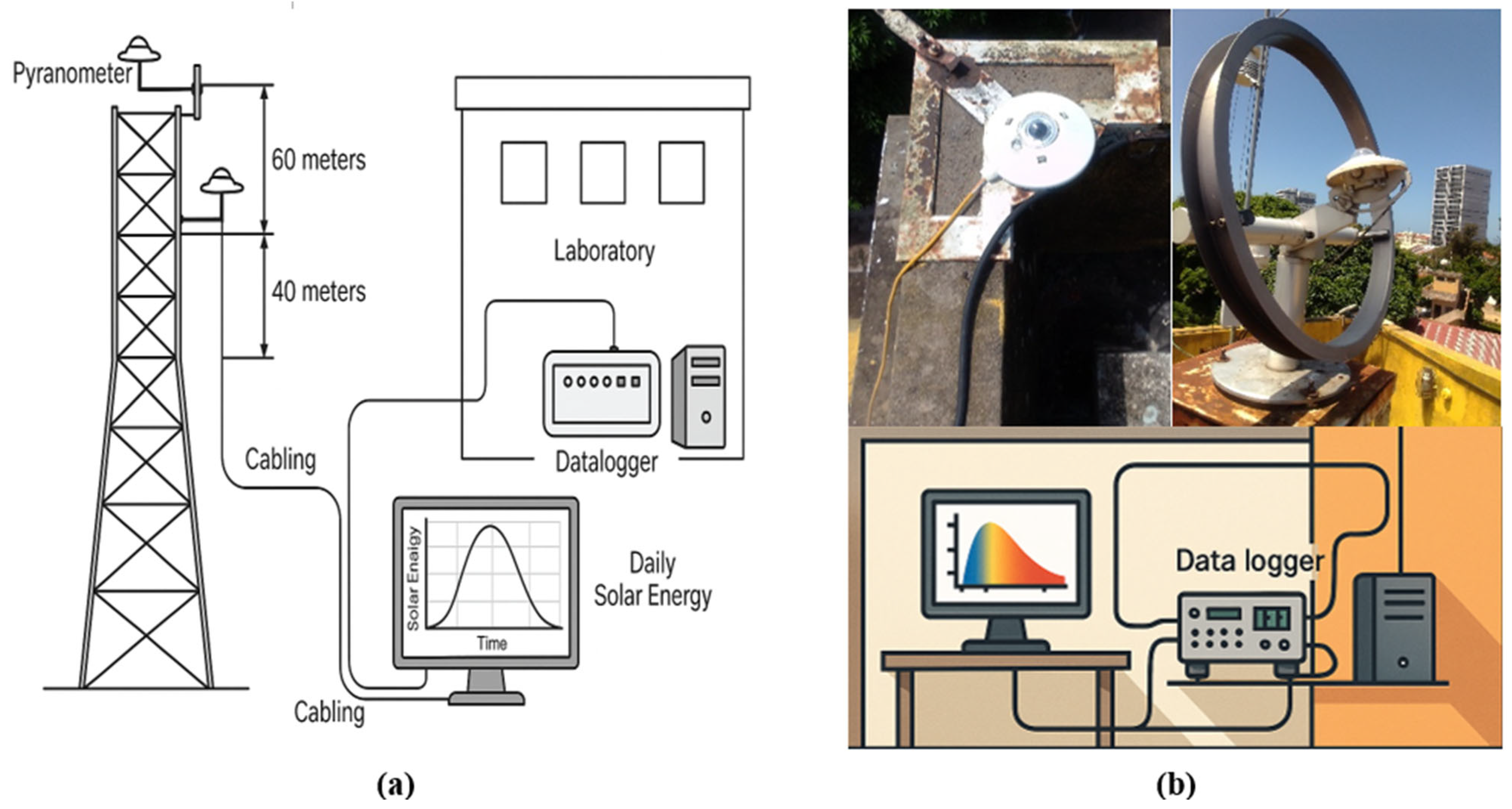
2.1. Data Collection and Processing
Setting Up and Running Data Collection Devices
2.2. Sample Size
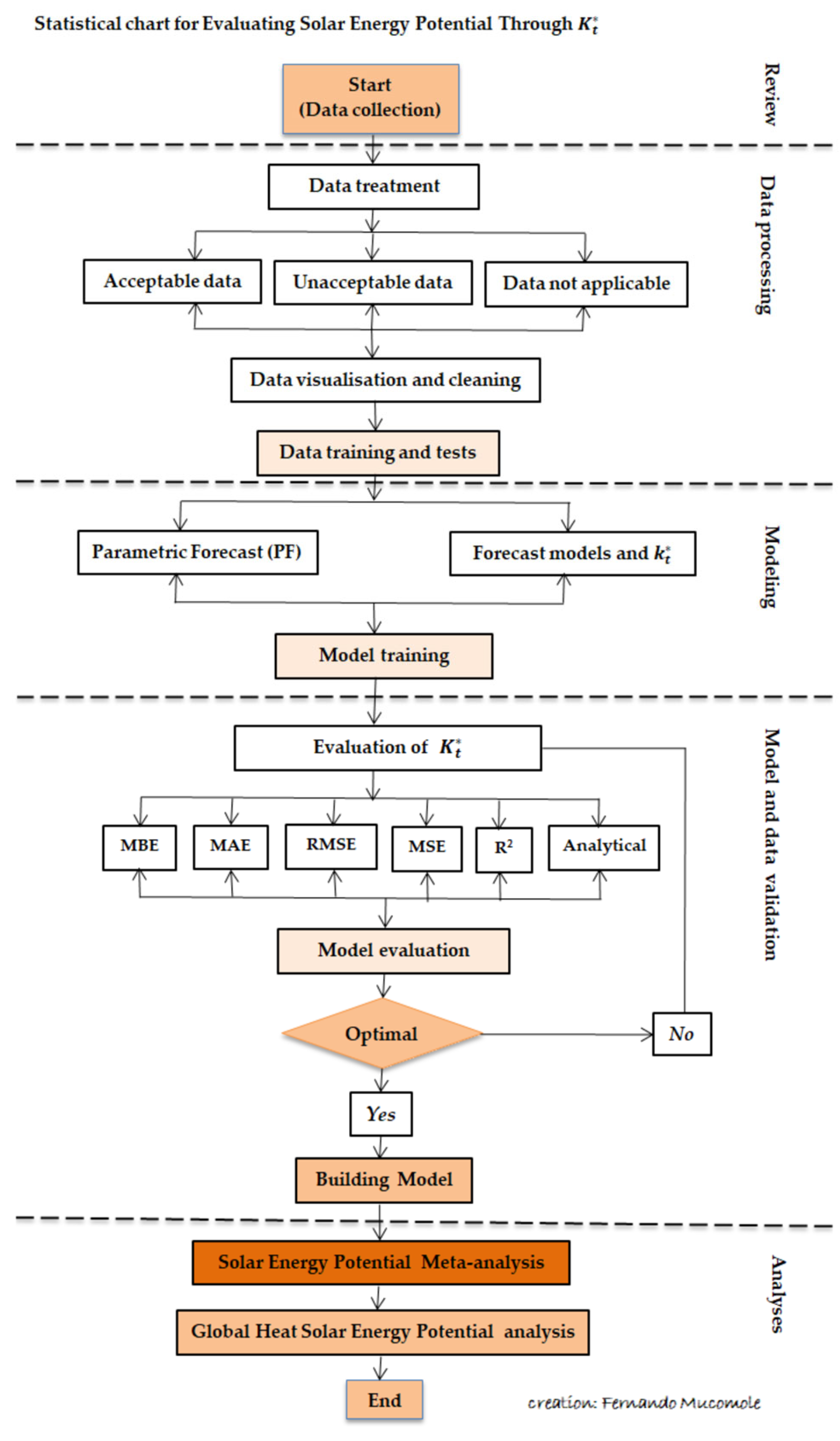
2.3. Procedural Execution Order for Solar Energy Analysis
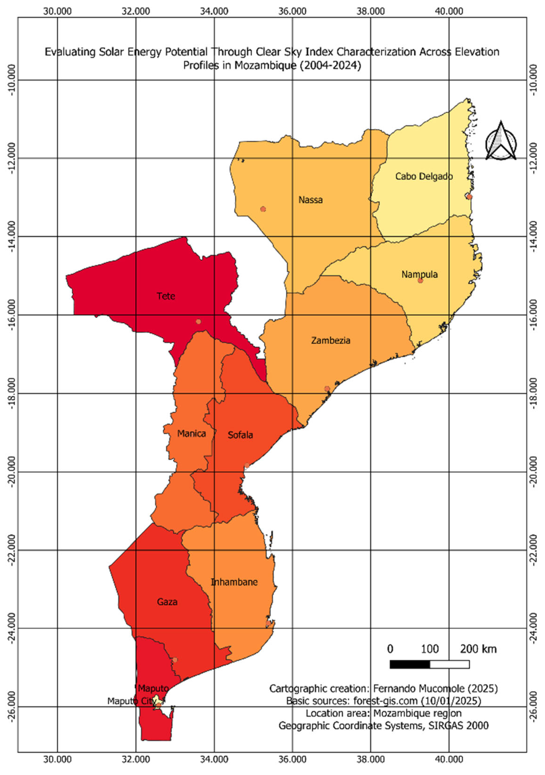
2.4. Study Area
2.5. Experimental Procedure
3. Results
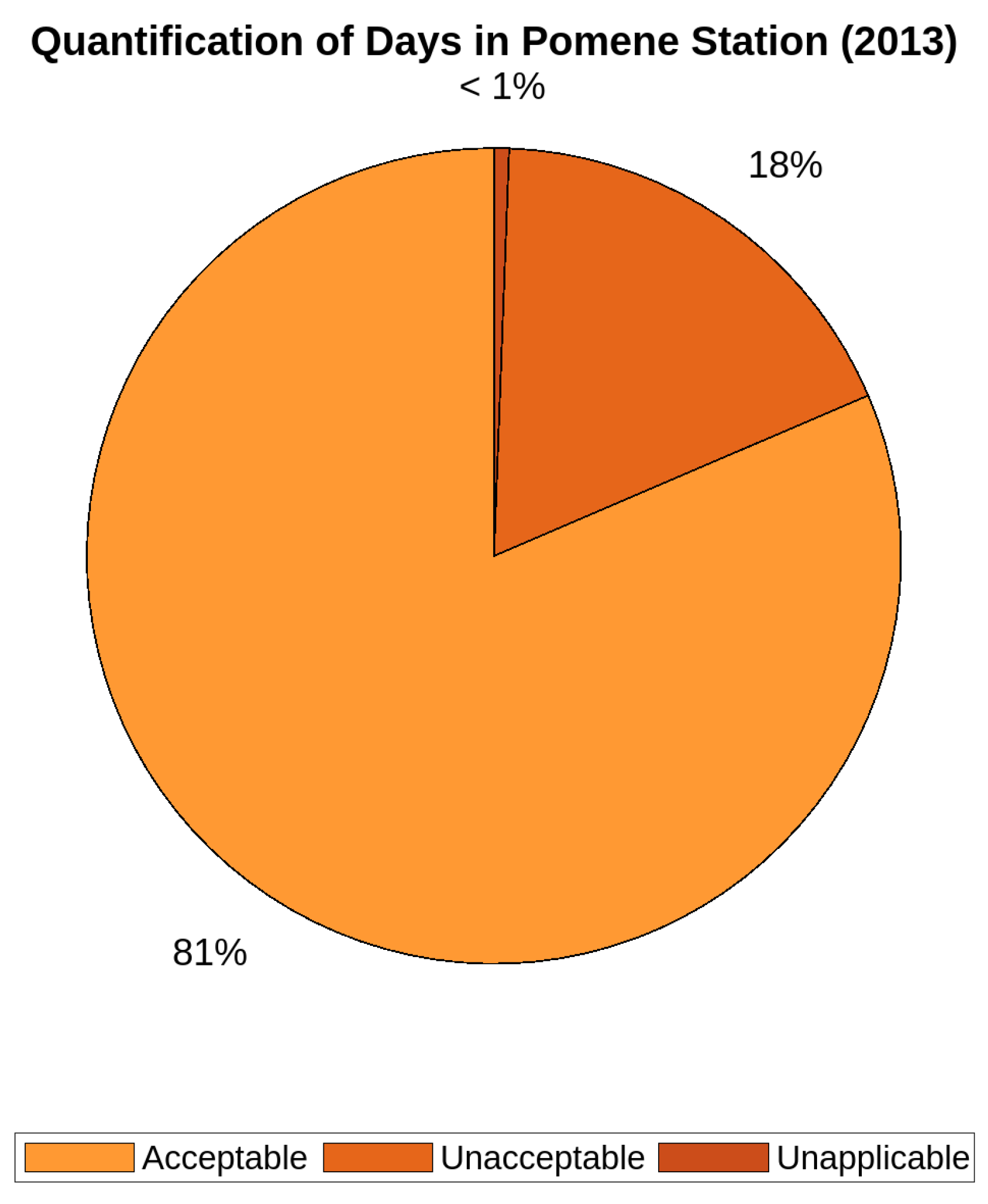
3.1. Percentage Estimate of Different Types of Days
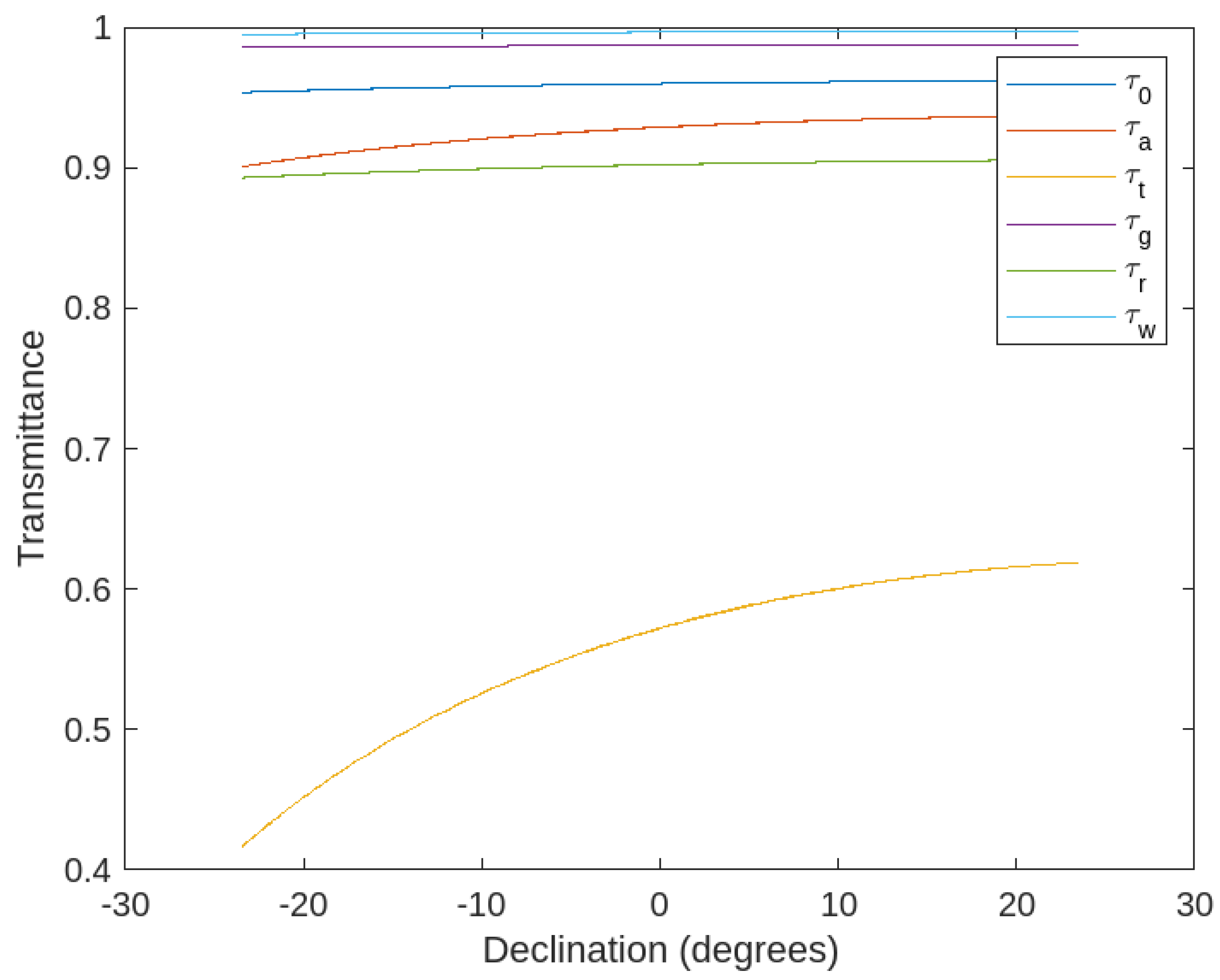
3.2. Casual Inference Factors for Determining Solar Energy
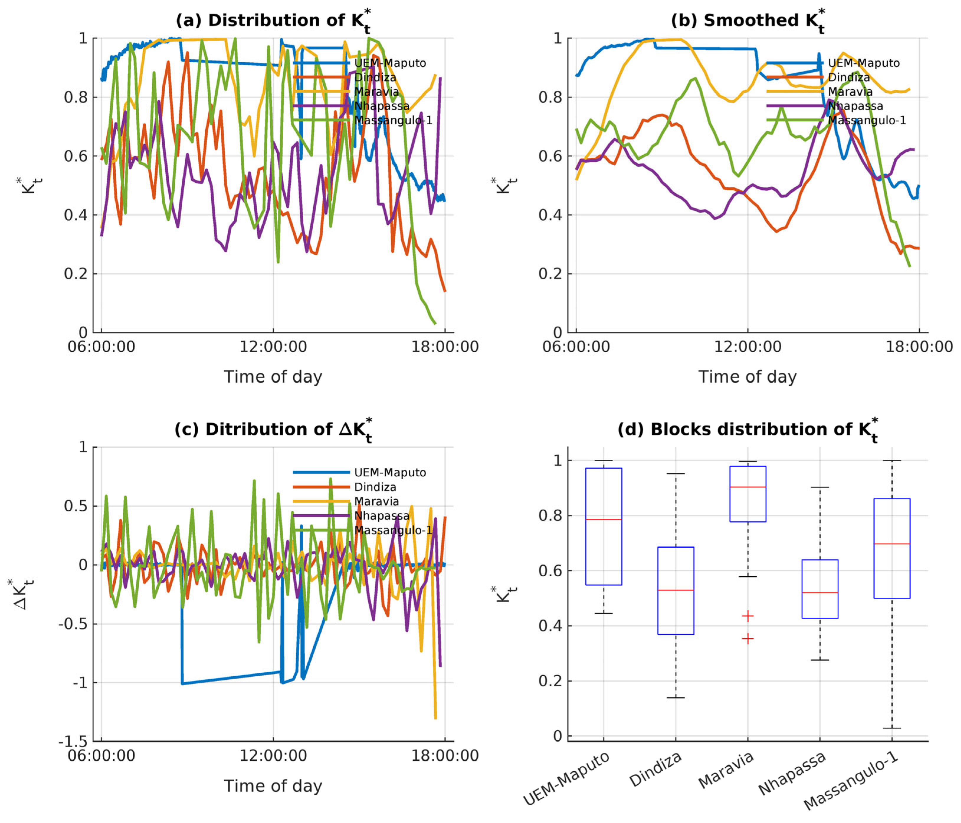
3.3. Characterization of the Variability in Intermediate Sky Days in Terms of Clear Sky Index
3.4. Variability of Intermediate Sky Days in Terms of Clear Sky Index Increments
3.5. Standard Deviation of the Variational of Clear Sky Index Coefficient Variation ()
3.6. Standard Deviation of the Variational Coefficient
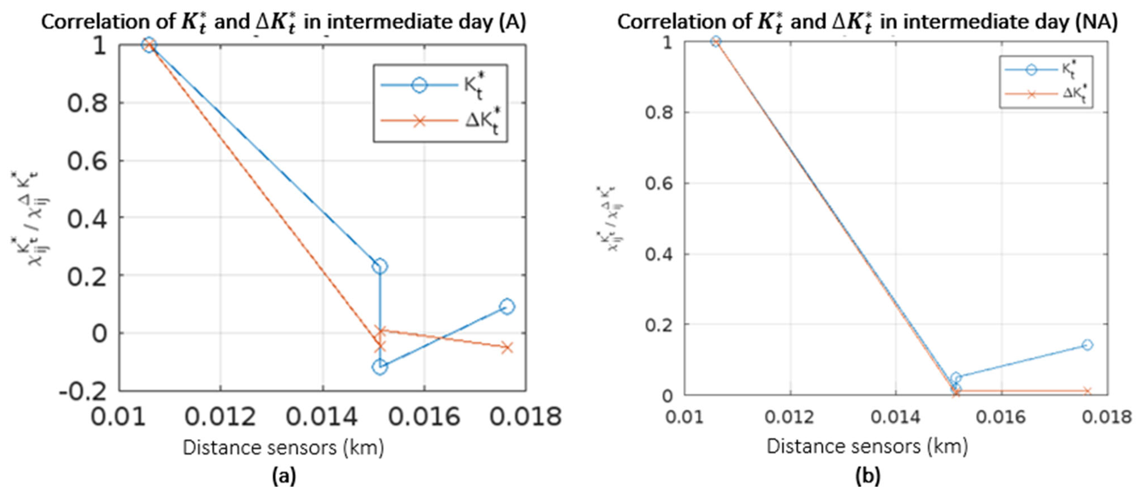
3.7. Connection of the Between Two Measurement Stations
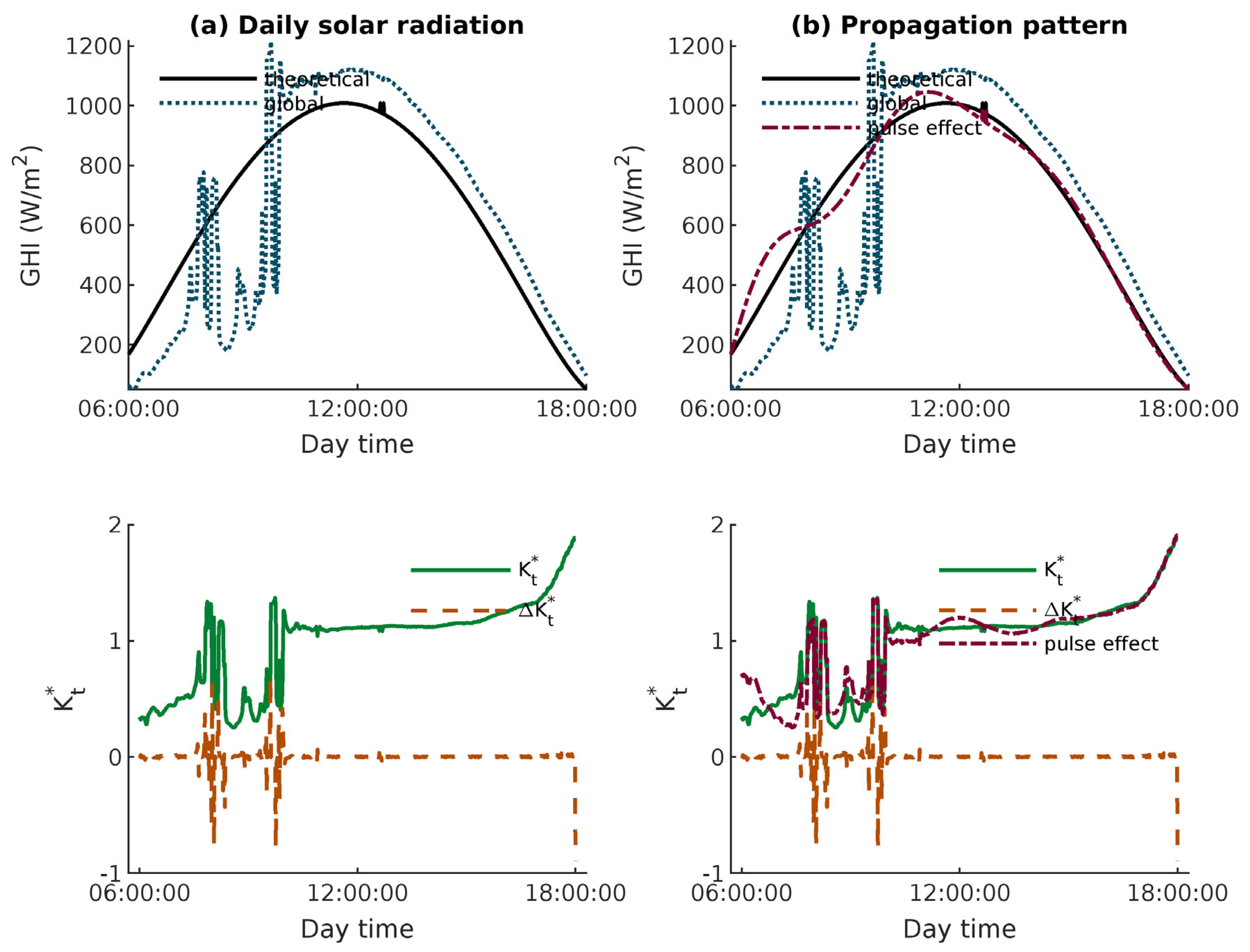
3.8. Incremental Analysis of High Fluctuations in the
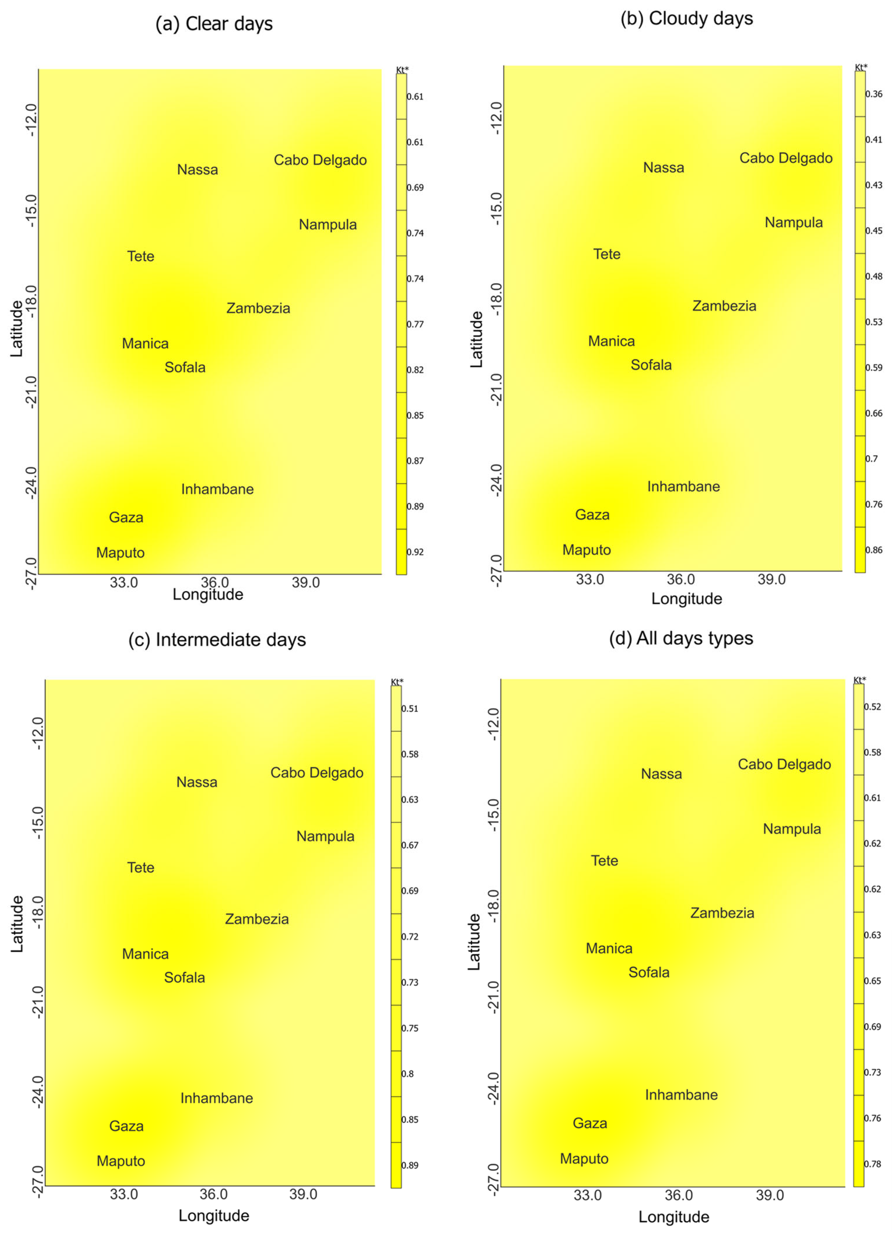
3.9. Solar Energy Potential Through , and Its Characterization Across Elevation Profiles in Mozambique
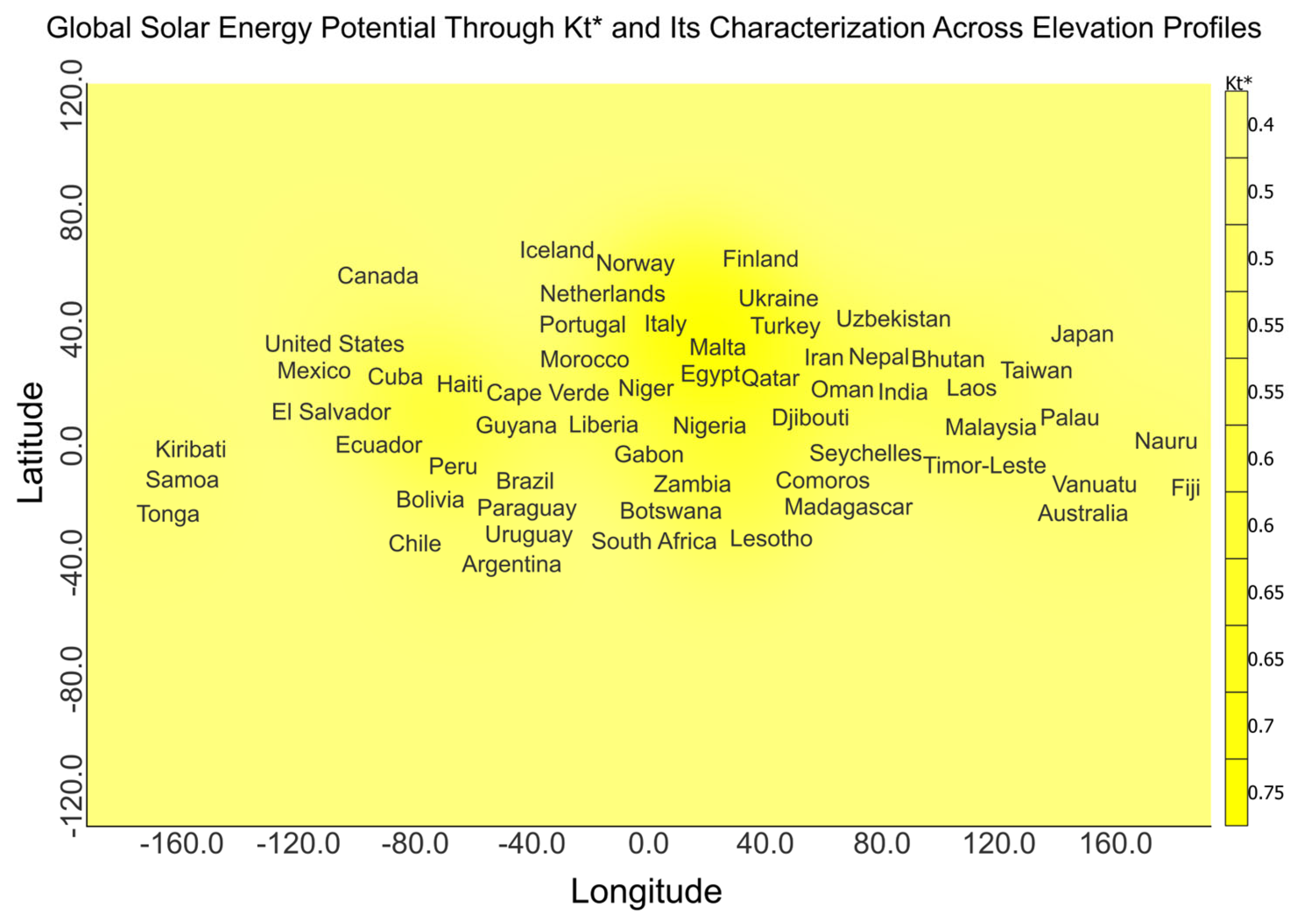
3.10. Global Solar Energy Potential Through and Its Characterization Across Elevation Profiles
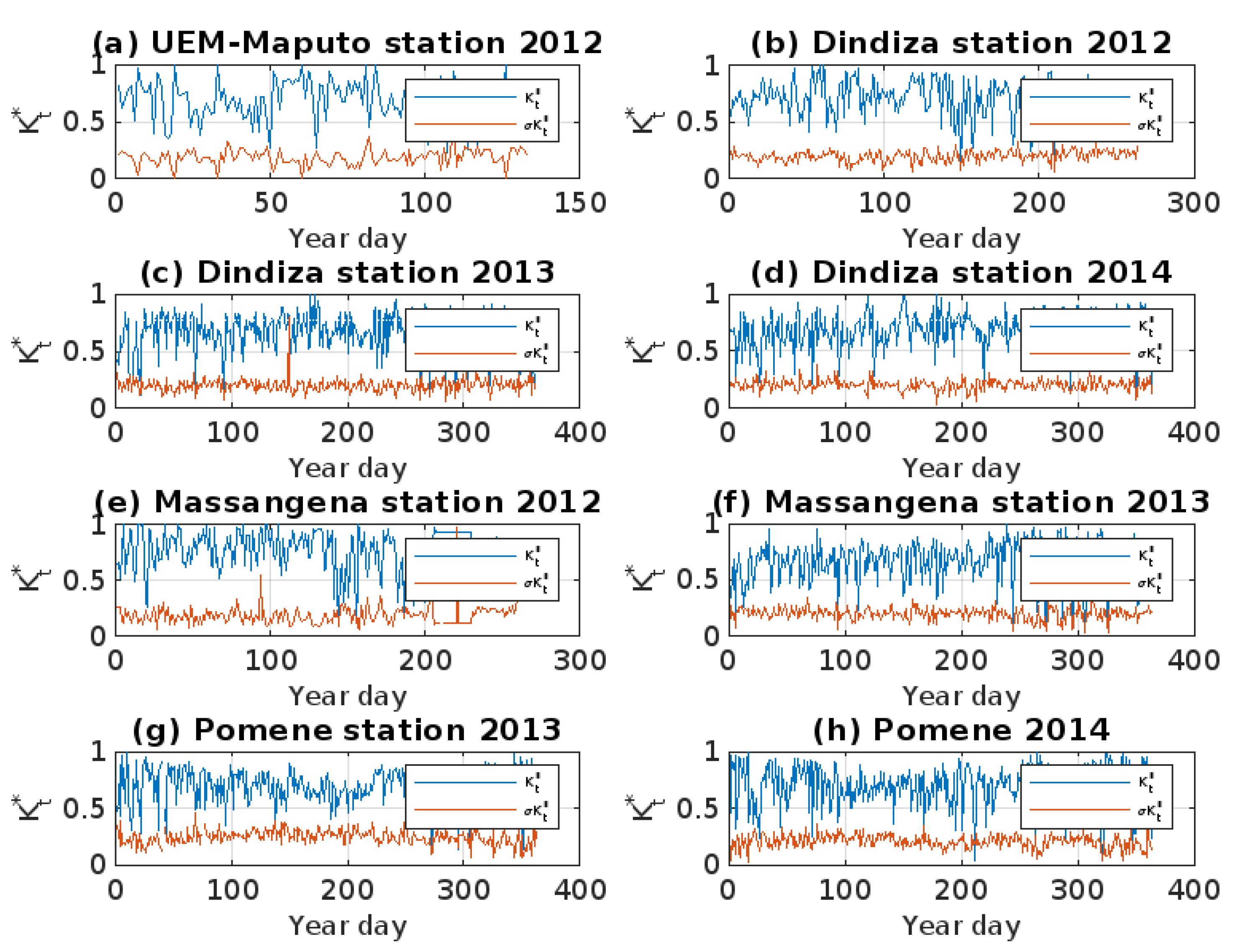
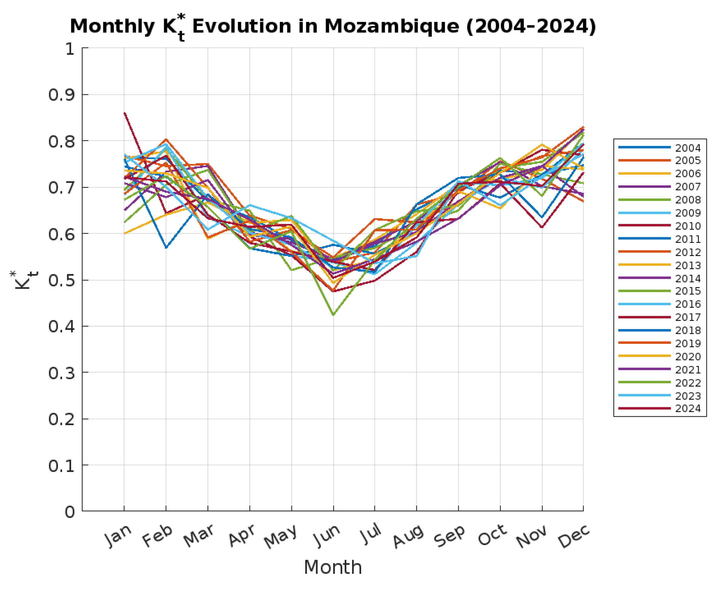
3.11. Analysis of the Annual Course of the Development and Trend of the Clear Sky Index
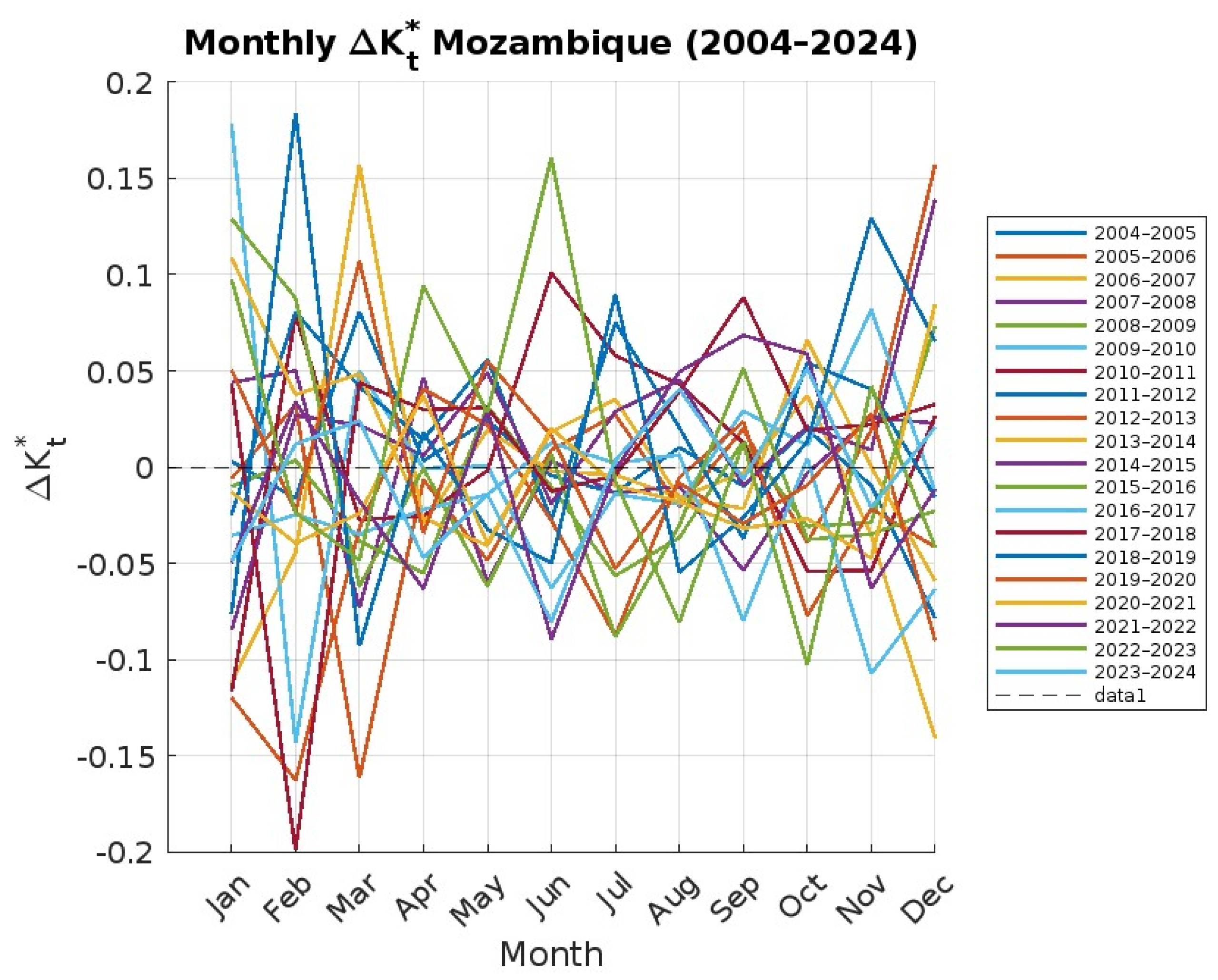
3.12. Analysis of the Annual Course of Development and Trend of Increases in the Clear Sky Index in Mozambique
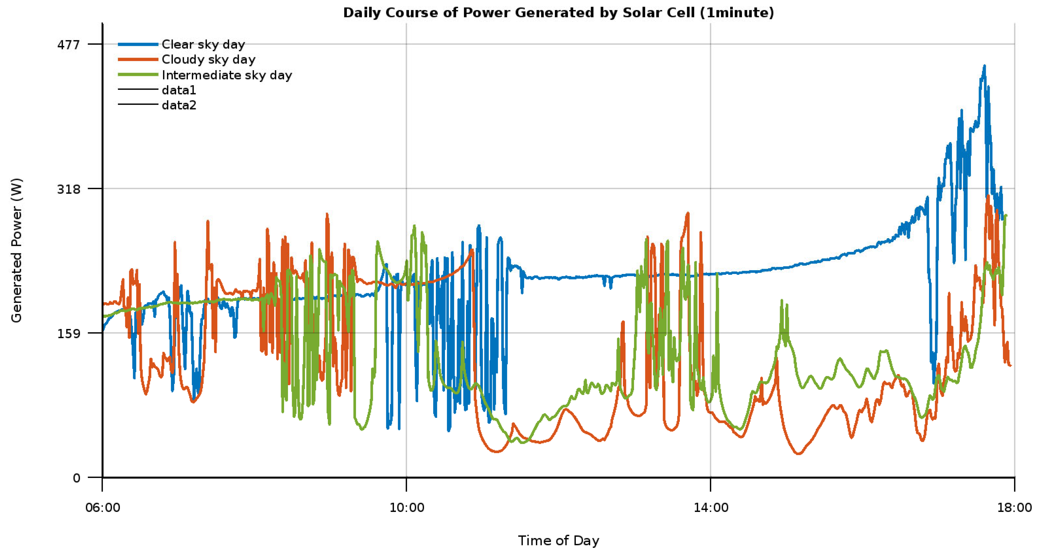
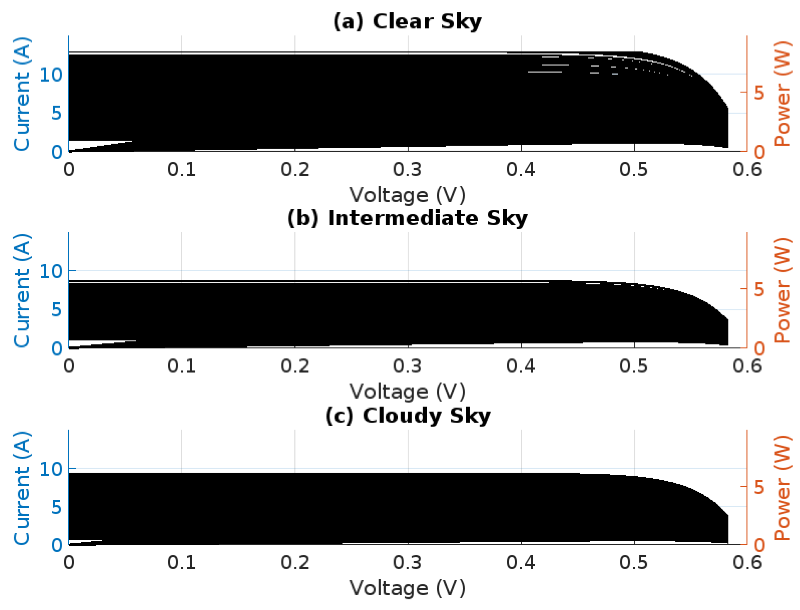
4. PV Generator Characteristics on Clear, Cloudy, and Intermediate Days in Mozambique Region
5. Discussion
6. Conclusions
Author Contributions
Funding
Institutional Review Board Statement
Informed Consent Statement
Data Availability Statement
Acknowledgments
Conflicts of Interest
Abbreviations
| DNI | Direct radiation |
| DHI | Diffuse radiation |
| PV | Photovoltaic |
| FUNAE | National Energy Fund |
| CS-OGET | Center of Excellence of Studies in Oil and Gas Engineering and Technology |
| CPE | Centre of Research in Energies |
| Extraterrestrial radiation on a horizontal surface | |
| Normal clear-sky DNI | |
| Normal clear-sky direct horizontal radiation | |
| Theoretical horizontal radiation | |
| GHI | Global radiation |
| INAM | National Institute of Meteorology |
| Clarity index | |
| Clear sky index | |
| Clear sky index variation | |
| KDE | Kernel density estimation |
| Probability density function | |
| Atmospheric transmittance | |
| Diffuse radiation from a clear sky on a horizontal surface | |
| Total | Calculated theoretical total radiation |
| UEM | Eduardo Mondlane University |
| Hour angle | |
| Standard deviation of | |
| IQR | Interquartile range |
| Whisker | |
| First quadrant | |
| Second quadrant | |
| Third quadrant | |
| Upper whisker | |
| Lower whisker | |
| E | East |
| S | South |
| N | North |
| W | West |
| EN | El Niño |
| LN | La Niña |
| Jan. | January |
| Feb. | February |
| Mar. | March |
| Apr. | April |
| May | May |
| June | June |
| July. | July |
| Aug. | August |
| Spt. | September |
| Oct. | October |
| Nov. | November |
| Dec. | December |
| Latitude given in degrees | |
| Declination angle | |
| Inclination angle | |
| Surface azimuth angle | |
| Hour angle | |
| Incidence angle | |
| Zenith angle | |
| Solar azimuth angle | |
| n | Number of days in accumulation, for each month of the year |
| Ozone | |
| Carbon dioxide |
References
- Duffie, J.A.; Beckman, W.A. Solar Engineering of Thermal Processes; Wiley and Sons: Hoboken, NJ, USA, 2013. [Google Scholar]
- Iqbal, M. An Introduction to Solar Radiation; Academic Press: Toronto, ON, Canada; New York, NY, USA, 1983. [Google Scholar]
- Perez, R.; Ineichen, P.; Moore, K.; Kmiecik, M.; Chain, C.; George, R.; Vignola, F. A new operational model for satellite-derived irradiances: Description and validation. Sol. Energy 2002, 73, 307–317. [Google Scholar] [CrossRef]
- IEA; IRENA; UNSD; World Bank; WHO. Tracking SDG 7: The Energy Progress Report; World Bank: Washington, DC, USA, 2023; Available online: https://cdn.who.int/media/docs/default-source/air-pollution-documents/air-quality-and-health/sdg7-report2023-full-report_web.pdf?sfvrsn=669e8626_3&download=true (accessed on 16 December 2023).
- Mucomole, F.V.; Silva, C.A.S.; Magaia, L.L. Temporal Variability of Solar Energy Availability in the Conditions of the Southern Region of Mozambique. Am. J. Energy Nat. Resour. 2023, 2, 27–50. [Google Scholar] [CrossRef]
- Vuilleumier, L.; Meyer, A.; Stöckli, R.; Wilbert, S.; Zarzalejo, L.F. Accuracy of satellite-derived solar direct irradiance in Southern Spain and Switzerland. Int. J. Remote Sens. 2020, 41, 8808–8838. [Google Scholar] [CrossRef]
- Lusi, A.R.; Orte, P.F.; Wolfram, E.; Orlando, J.I. Cloud classification through machine learning and global horizontal irradiance data analysis. Q. J. R. Meteorol. Soc. 2024, 150, 5435–5451. [Google Scholar] [CrossRef]
- Hu, L.; Brunsell, N.A. A new perspective to assess the urban heat island through remotely sensed atmospheric profiles. Remote Sens. Environ. 2015, 158, 393–406. [Google Scholar] [CrossRef]
- Al Garni, H.; Kassem, A.; Awasthi, A.; Komljenovic, D.; Al-Haddad, K. A multicriteria decision making approach for evaluating renewable power generation sources in Saudi Arabia. Sustain. Energy Technol. Assess. 2016, 16, 137–150. [Google Scholar] [CrossRef]
- Hammer, A.; Heinemann, D.; Hoyer, C.; Kuhlemann, R.; Lorenz, E.; Müller, R.; Beyer, H.G. Solar energy assessment using remote sensing technologies. Remote Sens. Environ. 2003, 86, 423–432. [Google Scholar] [CrossRef]
- Chauvin, R.; Nou, J.; Thil, S.; Grieu, S. Modelling the clear-sky intensity distribution using a sky imager. Sol. Energy 2015, 119, 1–17. [Google Scholar] [CrossRef]
- Dalton, G.J.; Lockington, D.A.; Baldock, T.E. Feasibility analysis of stand-alone renewable energy supply options for a large hotel. Renew. Energy 2008, 33, 1475–1490. [Google Scholar] [CrossRef]
- Chazdon, R.L.; Field, C.B. Photographic estimation of photosynthetically active radiation: Evaluation of a computerized technique. Oecologia 1987, 73, 525–532. [Google Scholar] [CrossRef]
- Compagnon, R. Solar and daylight availability in the urban fabric. Energy Build. 2004, 36, 321–328. [Google Scholar] [CrossRef]
- Widén, J.; Carpman, N.; Castellucci, V.; Lingfors, D.; Olauson, J.; Remouit, F.; Bergkvist, M.; Grabbe, M.; Waters, R. Variability assessment and forecasting of renewables: A review for solar, wind, wave and tidal resources. Renew. Sustain. Energy Rev. 2015, 44, 356–375. [Google Scholar] [CrossRef]
- Reinhart, C.F.; Wienold, J. The daylighting dashboard—A simulation-based design analysis for daylit spaces. Build. Environ. 2011, 46, 386–396. [Google Scholar] [CrossRef]
- Sreenath, S.; Sudhakar, K.; A.F., Y.; Solomin, E.; Kirpichnikova, I. Solar PV energy system in Malaysian airport: Glare analysis, general design and performance assessment. Energy Rep. 2020, 6, 698–712. [Google Scholar] [CrossRef]
- Urquhart, B.; Kurtz, B.; Dahlin, E.; Ghonima, M.; Shields, J.E.; Kleissl, J. Development of a sky imaging system for short-term solar power forecasting. Atmos. Meas. Tech. 2015, 8, 875–890. [Google Scholar] [CrossRef]
- Rumbayan, M.; Abudureyimu, A.; Nagasaka, K. Mapping of solar energy potential in Indonesia using artificial neural network and geographical information system. Renew. Sustain. Energy Rev. 2012, 16, 1437–1449. [Google Scholar] [CrossRef]
- Clifton, A.; Hodge, B.-M.; Draxl, C.; Badger, J.; Habte, A. Wind and solar resource data sets. WIREs Energy Environ. 2018, 7, e276. [Google Scholar] [CrossRef]
- Tiba, C.; Fraidenraich, N.; Gallegos, H.G.; Lyra, F.J.M. Solar energy resource assessment—Brazil. Renew. Energy 2002, 27, 383–400. [Google Scholar] [CrossRef]
- Mucomole, F.V.; Silva, C.A.S.; Magaia, L.L. Modeling Parametric Forecasts of Solar Energy over Time in the Mid-North Area of Mozambique. Energies 2025, 18, 1469. [Google Scholar] [CrossRef]
- Brent, A.C.; Hinkley, J.; Burmester, D.; Rayudu, R. Solar Atlas of New Zealand from satellite imagery. J. R. Soc. N. Z. 2020, 50, 572–583. Available online: https://www.tandfonline.com/doi/abs/10.1080/03036758.2020.1763409 (accessed on 15 March 2025). [CrossRef]
- Gastli, A.; Charabi, Y. Solar electricity prospects in Oman using GIS-based solar radiation maps. Renew. Sustain. Energy Rev. 2010, 14, 790–797. [Google Scholar] [CrossRef]
- Müller, J.; Mitra, I.; Mieslinger, T.; Meyer, R.; Chhatbar, K.; Gomathinayagam, S.; Giridhar, G. Towards building solar in India—A combined mapping and monitoring approach for creating a new solar atlas. Energy Sustain. Dev. 2017, 40, 31–40. [Google Scholar] [CrossRef]
- Abo-Zahhad, E.M.; Rashwan, A.; Salameh, T.; Hamid, A.K.; Faragalla, A.; El-Dein, A.Z.; Chen, Y.; Abdelhameed, E.H. Evaluation of solar PV-based microgrids viability utilizing single and multi-criteria decision analysis. Renew. Energy 2024, 221, 119713. [Google Scholar] [CrossRef]
- Wang, G.C.; Urquhart, B.; Kleissl, J. Cloud base height estimates from sky imagery and a network of pyranometers. Sol. Energy 2019, 184, 594–609. [Google Scholar] [CrossRef]
- Deo, R.C.; Wen, X.; Qi, F. A wavelet-coupled support vector machine model for forecasting global incident solar radiation using limited meteorological dataset. Appl. Energy 2016, 168, 568–593. [Google Scholar] [CrossRef]
- Wenham, S.R.; Green, M.A.; Watt, M.E.; Corkish, R.; Sproul, A. (Eds.) Applied Photovoltaics, 3rd ed.; Routledge: London, UK, 2011. [Google Scholar] [CrossRef]
- Gueymard, C.A. Clear-sky irradiance predictions for solar resource mapping and large-scale applications: Improved validation methodology and detailed performance analysis of 18 broadband radiative models. Sol. Energy 2012, 86, 2145–2169. [Google Scholar] [CrossRef]
- Huld, T.; Müller, R.; Gambardella, A. A new solar radiation database for estimating PV performance in Europe and Africa. Sol. Energy 2012, 86, 1803–1815. [Google Scholar] [CrossRef]
- Archer, C.L.; Monache, L.D.; Rife, D.L. Airborne wind energy: Optimal locations and variability. Renew. Energy 2014, 64, 180–186. [Google Scholar] [CrossRef]
- Marquez, R.; Coimbra, C.F.M. Forecasting of global and direct solar irradiance using stochastic learning methods, ground experiments and the NWS database. Sol. Energy 2011, 85, 746–756. [Google Scholar] [CrossRef]
- Lorenz, E.; Guthke, P.; Dittmann, A.; Holland, N.; Herzberg, W.; Karalus, S.; Müller, B.; Braun, C.; Heydenreich, W.; Saint-Drenan, Y.-M. High resolution measurement network of global horizontal and tilted solar irradiance in southern Germany with a new quality control scheme. Sol. Energy 2022, 231, 593–606. [Google Scholar] [CrossRef]
- Antonanzas, J.; Osorio, N.; Escobar, R.; Urraca, R.; Martinez-de-Pison, F.J.; Antonanzas-Torres, F. Review of photovoltaic power forecasting. Sol. Energy 2016, 136, 78–111. [Google Scholar] [CrossRef]
- Wang, L.; Lu, Y.; Wang, Z.; Li, H.; Zhang, M. Hourly solar radiation estimation and uncertainty quantification using hybrid models. Renew. Sustain. Energy Rev. 2024, 202, 114727. [Google Scholar] [CrossRef]
- Hock, R. A distributed temperature-index ice- and snowmelt model including potential direct solar radiation. J. Glaciol. 1999, 45, 101–111. [Google Scholar] [CrossRef]
- Tassaddiq, A.; Qureshi, S.; Soomro, A.; Hincal, E.; Shaikh, A.A. A new continuous hybrid block method with one optimal intrastep point through interpolation and collocation. Fixed Point Theory Algorithms Sci. Eng. 2022, 2022, 1–17. [Google Scholar] [CrossRef]
- Trapero, J.R.; Kourentzes, N.; Martin, A. Short-term solar irradiation forecasting based on Dynamic Harmonic Regression. Energy 2015, 84, 289–295. [Google Scholar] [CrossRef]
- El-Sebaii, A.A.; Trabea, A.A. Estimation of horizontal diffuse solar radiation in Egypt. Energy Convers. Manag. 2003, 44, 2471–2482. [Google Scholar] [CrossRef]
- Kumar, V.; Hundal, B.S.; Syan, A.S. Factors affecting customers’ attitude towards solar energy products. Int. J. Bus. Innov. Res. 2020, 21, 271–293. [Google Scholar] [CrossRef]
- Said, Y.; Alanazi, A. AI-based solar energy forecasting for smart grid integration. Neural Comput. Appl. 2023, 35, 8625–8634. [Google Scholar] [CrossRef]
- Ozoegwu, C.G. Artificial neural network forecast of monthly mean daily global solar radiation of selected locations based on time series and month number. J. Clean. Prod. 2019, 216, 1–13. [Google Scholar] [CrossRef]
- Ledmaoui, Y.; El Maghraoui, A.; El Aroussi, M.; Saadane, R.; Chebak, A.; Chehri, A. Forecasting solar energy production: A comparative study of machine learning algorithms. Energy Rep. 2023, 10, 1004–1012. [Google Scholar] [CrossRef]
- Deo, R.C.; Ahmed, A.M.; Casillas-Pérez, D.; Pourmousavi, S.A.; Segal, G.; Yu, Y.; Salcedo-Sanz, S. Cloud cover bias correction in numerical weather models for solar energy monitoring and forecasting systems with kernel ridge regression. Renew. Energy 2023, 203, 113–130. [Google Scholar] [CrossRef]
- Utlu, Z.; Hepbasli, A. Analyzing the Energy Utilization Efficiency of Renewable Energy Resources. Part 1: Energy Analysis Method. Energy Sources Part B Econ. Plan. Policy 2006, 1, 341–353. [Google Scholar] [CrossRef]
- Jiang, D.; Zhuang, D.; Huang, Y.; Wang, J.; Fu, J. Evaluating the spatio-temporal variation of China’s offshore wind resources based on remotely sensed wind field data. Renew. Sustain. Energy Rev. 2013, 24, 142–148. [Google Scholar] [CrossRef]
- González-Rodríguez, L.; Cabrera-Reina, A.; Rosas, J.; Volke, M.; Marzo, A. Characterization of solar-derivate ultraviolet radiation for water solar treatment applications. Renew. Energy 2024, 233, 121078. [Google Scholar] [CrossRef]
- Sarver, T.; Al-Qaraghuli, A.; Kazmerski, L.L. A comprehensive review of the impact of dust on the use of solar energy: History, investigations, results, literature, and mitigation approaches. Renew. Sustain. Energy Rev. 2013, 22, 698–733. [Google Scholar] [CrossRef]
- Bódis, K.; Kougias, I.; Jäger-Waldau, A.; Taylor, N.; Szabó, S. A high-resolution geospatial assessment of the rooftop solar photovoltaic potential in the European Union. Renew. Sustain. Energy Rev. 2019, 114, 109309. [Google Scholar] [CrossRef]
- Šúri, M.; Hofierka, J. A New GIS-based Solar Radiation Model and Its Application to Photovoltaic Assessments. Trans. GIS 2004, 8, 175–190. [Google Scholar] [CrossRef]
- Huebert, B.J.; Bates, T.; Russell, P.B.; Shi, G.; Kim, Y.J.; Kawamura, K.; Carmichael, G.; Nakajima, T. An overview of ACE-Asia: Strategies for quantifying the relationships between Asian aerosols and their climatic impacts. J. Geophys. Res. Atmospheres 2003, 108, 8633. [Google Scholar] [CrossRef]
- Hamad, J.; Ahmad, M.; Zeeshan, M. Solar energy resource mapping, site suitability and techno-economic feasibility analysis for utility scale photovoltaic power plants in Afghanistan. Energy Convers. Manag. 2024, 303, 118188. [Google Scholar] [CrossRef]
- Dehshiri, S.J.H.; Amiri, M.; Mostafaeipour, A.; Le, T. Evaluation of renewable energy projects based on sustainability goals using a hybrid pythagorean fuzzy-based decision approach. Energy 2024, 297, 131272. [Google Scholar] [CrossRef]
- Santos, T.; Gomes, N.; Freire, S.; Brito, M.C.; Santos, L.; Tenedório, J.A. Applications of solar mapping in the urban environment. Appl. Geogr. 2014, 51, 48–57. [Google Scholar] [CrossRef]
- Perez, R.; Ineichen, P.; Seals, R.; Michalsky, J.; Stewart, R. Modeling daylight availability and irradiance components from direct and global irradiance. Sol. Energy 1990, 44, 271–289. [Google Scholar] [CrossRef]
- Kapica, J.; Canales, F.A.; Jurasz, J. Global atlas of solar and wind resources temporal complementarity. Energy Convers. Manag. 2021, 246, 114692. [Google Scholar] [CrossRef]
- Prăvălie, R.; Patriche, C.; Bandoc, G. Spatial assessment of solar energy potential at global scale. A geographical approach. J. Clean. Prod. 2019, 209, 692–721. [Google Scholar] [CrossRef]
- Hoff, T.E.; Perez, R. Quantifying PV power Output Variability. Sol. Energy 2010, 84, 1782–1793. [Google Scholar] [CrossRef]
- Freitas, S.; Catita, C.; Redweik, P.; Brito, M.C. Modelling solar potential in the urban environment: State-of-the-art review. Renew. Sustain. Energy Rev. 2015, 41, 915–931. [Google Scholar] [CrossRef]
- Bourbia, F.; Boucheriba, F. Impact of street design on urban microclimate for semi arid climate (Constantine). Renew. Energy 2010, 35, 343–347. [Google Scholar] [CrossRef]
- Angelis-Dimakis, A.; Biberacher, M.; Dominguez, J.; Fiorese, G.; Gadocha, S.; Gnansounou, E.; Guariso, G.; Kartalidis, A.; Panichelli, L.; Pinedo, I.; et al. Methods and tools to evaluate the availability of renewable energy sources. Renew. Sustain. Energy Rev. 2011, 15, 1182–1200. [Google Scholar] [CrossRef]
- Wienold, J.; Christoffersen, J. Evaluation methods and development of a new glare prediction model for daylight environments with the use of CCD cameras. Energy Build. 2006, 38, 743–757. [Google Scholar] [CrossRef]
- Coimbra, C.F.M. Energy Meteorology for the Evaluation of Solar Farm Thermal Impacts on Desert Habitats. Adv. Atmos. Sci. 2025, 42, 313–326. [Google Scholar] [CrossRef]
- Baret, F.; Guyot, G. Potentials and limits of vegetation indices for LAI and APAR assessment. Remote Sens. Environ. 1991, 35, 161–173. [Google Scholar] [CrossRef]
- Zhang, Y.; Chen, L. Estimation of Daily Average Shortwave Solar Radiation under Clear-Sky Conditions by the Spatial Downscaling and Temporal Extrapolation of Satellite Products in Mountainous Areas. Remote Sens. 2022, 14, 2710. [Google Scholar] [CrossRef]
- Lohmann, G.M. Irradiance Variability Quantification and Small-Scale Averaging in Space and Time: A Short Review. Atmosphere 2018, 9, 264. [Google Scholar] [CrossRef]
- van Haaren, R.; Fthenakis, V. GIS-based wind farm site selection using spatial multi-criteria analysis (SMCA): Evaluating the case for New York State. Renew. Sustain. Energy Rev. 2011, 15, 3332–3340. [Google Scholar] [CrossRef]
- Qiu, L.; He, L.; Lu, H.; Liang, D. Pumped hydropower storage potential and its contribution to hybrid renewable energy co-development: A case study in the Qinghai-Tibet Plateau. J. Energy Storage 2022, 51, 104447. [Google Scholar] [CrossRef]
- Müller, R.W.; Dagestad, K.F.; Ineichen, P.; Schroedter-Homscheidt, M.; Cros, S.; Dumortier, D.; Kuhlemann, R.; Olseth, J.A.; Piernavieja, G.; Reise, C.; et al. Rethinking satellite-based solar irradiance modelling: The SOLIS clear-sky module. Remote Sens. Environ. 2004, 91, 160–174. [Google Scholar] [CrossRef]
- Lohmann, G.M.; Monahan, A.H. Effects of temporal averaging on short-term irradiance variability under mixed sky conditions. Atmospheric Measurement Techn. 2018, 5, 3131–3144. [Google Scholar] [CrossRef]
- Perez, M.J.R.; Fthenakis, V.M. On the spatial decorrelation of stochastic solar resource variability at long timescales. Sol. Energy 2015, 117, 46–58. [Google Scholar] [CrossRef]
- Magaia, L.L.; Silva, C.A.S.; Magaia, L.L. Long–Term Inference of Solar Energy Accessibility through Short-Term Measurements: Experimental Sampling Descriptor. Preprints 2025, 21, 2025041674. [Google Scholar] [CrossRef]
- Yang, K.; He, J.; Tang, W.; Qin, J.; Cheng, C.C.K. On downward shortwave and longwave radiations over high altitude regions: Observation and modeling in the Tibetan Plateau. Agric. For. Meteorol. 2010, 150, 38–46. [Google Scholar] [CrossRef]
- Ahmed Mohammed, A.; Aung, Z. Ensemble Learning Approach for Probabilistic Forecasting of Solar Power Generation. Energies 2016, 9, 1017. [Google Scholar] [CrossRef]
- Joshi, B.; Kay, M.; Copper, J.K.; Sproul, A.B. Evaluation of solar irradiance forecasting skills of the Australian Bureau of Meteorology’s ACCESS models. Sol. Energy 2019, 188, 386–402. [Google Scholar] [CrossRef]
- Urraca, R.; Gracia-Amillo, A.M.; Huld, T.; Martinez-De-Pison, F.J.; Trentmann, J.; Lindfors, A.V.; Riihelä, A.; Sanz-Garcia, A. Quality control of global solar radiation data with satellite-based products. Sol. Energy 2017, 158, 49–62. [Google Scholar] [CrossRef]
- Ameur, A.; Berrada, A.; Loudiyi, K.; Aggour, M. Forecast modeling and performance assessment of solar PV systems. J. Clean. Prod. 2020, 267, 122167. [Google Scholar] [CrossRef]
- Haurant, P.; Muselli, M.; Gaillard, L.; Oberti, P. A new methodology to analyse and optimize territorial compensations of solar radiation intermittency: A case study in Corsica Island (France). Renew. Energy 2022, 185, 598–610. [Google Scholar] [CrossRef]
- Woodruff, D.L.; Deride, J.; Staid, A.; Watson, J.-P.; Slevogt, G.; Silva-Monroy, C. Constructing probabilistic scenarios for wide-area solar power generation. Sol. Energy 2018, 160, 153–167. [Google Scholar] [CrossRef]
- Wald, L. Basics in Solar Radiation at Earth Surface; O.I.E.—Observation, Impacts, Energy Center: Sophia Antipolis, France, 2018. [Google Scholar]
- Wan, C.; Zhao, J.; Song, Y.; Xu, Z.; Lin, J.; Hu, Z. Photovoltaic and solar power forecasting for smart grid energy management. CSEE J. Power Energy Syst. 2015, 1, 38–46. [Google Scholar] [CrossRef]
- Avila, S.; Deniau, Y.; Sorman, A.H.; McCarthy, J. (Counter)mapping renewables: Space, justice, and politics of wind and solar power in Mexico. Environ. Plan. E 2022, 5, 1056–1085. [Google Scholar] [CrossRef]
- Fish, C.S.; Calvert, K. An Analysis of Interactive Solar Energy Web Maps for Urban Energy Sustainability. Cartogr. Perspect. 2016, 85, 5–22. [Google Scholar] [CrossRef]
- Pillot, B.; Muselli, M.; Poggi, P.; Haurant, P.; Hared, I. Solar energy potential atlas for planning energy system off-grid electrification in the Republic of Djibouti. Energy Convers. Manag. 2013, 69, 131–147. [Google Scholar] [CrossRef]
- Martinez, A.; Iglesias, G. Hybrid wind-solar energy resources mapping in the European Atlantic. Sci. Total Environ. 2024, 928, 172501. [Google Scholar] [CrossRef] [PubMed]
- Charles, R.G.; Davies, M.L.; Douglas, P.; Hallin, I.L.; Mabbett, I. Sustainable energy storage for solar home systems in rural Sub-Saharan Africa—A comparative examination of lifecycle aspects of battery technologies for circular economy, with emphasis on the South African context. Energy 2019, 166, 1207–1215. [Google Scholar] [CrossRef]
- Belušić, A.; Prtenjak, M.T.; Güttler, I.; Ban, N.; Leutwyler, D.; Schär, C. Near-surface wind variability over the broader Adriatic region: Insights from an ensemble of regional climate models. Clim. Dyn. 2018, 50, 4455–4480. [Google Scholar] [CrossRef]
- Batra, N.; Islam, S.; Venturini, V.; Bisht, G.; Jiang, L. Estimation and comparison of evapotranspiration from MODIS and AVHRR sensors for clear sky days over the Southern Great Plains. Remote Sens. Environ. 2006, 103, 1–15. [Google Scholar] [CrossRef]
- Lolli, S.; Khor, W.Y.; Matjafri, M.Z.; Lim, H.S. Monsoon Season Quantitative Assessment of Biomass Burning Clear-Sky Aerosol Radiative Effect at Surface by Ground-Based Lidar Observations in Pulau Pinang, Malaysia in 2014. Remote Sens. 2019, 11, 2660. [Google Scholar] [CrossRef]
- Didavi, A.B.K.; Agbokpanzo, R.G.; Agbomahena, M. Comparative study of Decision Tree, Random Forest and XGBoost performance in forecasting the power output of a photovoltaic system. In Proceedings of the 2021 4th International Conference on Bio-Engineering for Smart Technologies (BioSMART), Paris/Creteil, France, 8–10 December 2021; pp. 1–5. [Google Scholar] [CrossRef]
- Kurtgoz, Y.; Deniz, E. Chapter 1.8—Comparison of ANN, Regression Analysis, and ANFIS Models in Estimation of Global Solar Radiation for Different Climatological Locations. In Exergetic, Energetic and Environmental Dimensions; Dincer, I., Colpan, C.O., Kizilkan, O., Eds.; Academic Press: Cambridge, MA, USA, 2018; pp. 133–148. [Google Scholar] [CrossRef]
- Jerez, S.; Tobin, I.; Turco, M.; Jiménez-Guerrero, P.; Vautard, R.; Montávez, J.P. Future changes, or lack thereof, in the temporal variability of the combined wind-plus-solar power production in Europe. Renew. Energy 2019, 139, 251–260. [Google Scholar] [CrossRef]
- Jerez, S.; Trigo, R.M.; Sarsa, A.; Lorente-Plazas, R.; Pozo-Vázquez, D.; Montávez, J.P. Spatio-temporal Complementarity between Solar and Wind Power in the Iberian Peninsula. Energy Procedia 2013, 40, 48–57. [Google Scholar] [CrossRef]
- Yordanov, I.; Velikova, V.; Tsonev, T. Plant Responses to Drought, Acclimation, and Stress Tolerance. Photosynthetica 2012, 38, 171–186. [Google Scholar] [CrossRef]
- Ratti, C.; Raydan, D.; Steemers, K. Building form and environmental performance: Archetypes, analysis and an arid climate. Energy Build. 2003, 35, 49–59. [Google Scholar] [CrossRef]
- Aryaputera, A.W.; Yang, D.; Zhao, L.; Walsh, W.M. Very short-term irradiance forecasting at unobserved locations using spatio-temporal kriging. Sol. Energy 2015, 122, 1266–1278. [Google Scholar] [CrossRef]
- Paoli, C.; Voyant, C.; Muselli, M.; Nivet, M.-L. Forecasting of preprocessed daily solar radiation time series using neural networks. Sol. Energy 2010, 84, 2146–2160. [Google Scholar] [CrossRef]
- Takilalte, A.; Harrouni, S.; Yaiche, M.R.; Mora-López, L. New approach to estimate 5-min global solar irradiation data on tilted planes from horizontal measurement. Renew. Energy 2020, 145, 2477–2488. [Google Scholar] [CrossRef]
- Trindade, A.; Cordeiro, L.C. Synthesis of Solar Photovoltaic Systems: Optimal Sizing Comparison. In Software Verification; Christakis, M., Polikarpova, N., Duggirala, P.S., Schrammel, P., Eds.; Lecture Notes in Computer Science; Springer International Publishing: Cham, Switzerland, 2020; Volume 12549, pp. 87–105. [Google Scholar] [CrossRef]
- Chow, C.W.; Belongie, S.; Kleissl, J. Cloud motion and stability estimation for intra-hour solar forecasting. Sol. Energy 2015, 115, 645–655. [Google Scholar] [CrossRef]
- Ferry, A.; Thebault, M.; Nérot, B.; Berrah, L.; Ménézo, C. Modeling and analysis of rooftop solar potential in highland and lowland territories: Impact of mountainous topography. Sol. Energy 2024, 275, 112632. [Google Scholar] [CrossRef]
- Pandey, C.K.; Katiyar, A.K. Solar Radiation: Models and Measurement Techniques. J. Energy 2013, 2013, 305207. [Google Scholar] [CrossRef]
- Obiwulu, A.U.; Erusiafe, N.; Olopade, M.A.; Nwokolo, S.C. Modeling and estimation of the optimal tilt angle, maximum incident solar radiation, and global radiation index of the photovoltaic system. Heliyon 2022, 8, e09598. [Google Scholar] [CrossRef]
- van der Meer, D.W.; Munkhammar, J.; Widén, J. Probabilistic forecasting of solar power, electricity consumption and net load: Investigating the effect of seasons, aggregation and penetration on prediction intervals. Sol. Energy 2018, 171, 397–413. [Google Scholar] [CrossRef]
- Rehman, S.; Bader, M.A.; Al-Moallem, S.A. Cost of solar energy generated using PV panels. Renew. Sustain. Energy Rev. 2007, 11, 1843–1857. [Google Scholar] [CrossRef]
- JRC Photovoltaic Geographical Information System (PVGIS)—European Commission. Available online: https://re.jrc.ec.europa.eu/pvg_tools/en/#MR (accessed on 4 April 2025).
- Meteonorm Version 8—Meteonorm 2025. Available online: https://meteonorm.com/meteonorm-version-8 (accessed on 19 June 2024).
- Aerosol Optical Depth Retrieval over the NASA Stennis Space Center: MTI, MODIS, and AERONET | IEEE Journals & Magazine | IEEE Xplore. Available online: https://ieeexplore.ieee.org/abstract/document/1499013 (accessed on 6 September 2024).
- NOAA AVHRR Derived Aerosol Optical Depth over Land—Hauser—2005—Journal of Geophysical Research: Atmospheres—Wiley Online Library. Available online: https://agupubs.onlinelibrary.wiley.com/doi/full/10.1029/2004JD005439 (accessed on 4 September 2024).
- INAM (National Meteorology Institute of Mozambique). 2024. Available online: https://www.inam.gov.mz/index.php/pt/ (accessed on 5 May 2023).
- FUNAE (National Energy Fund of Mozambique). 2023. Available online: https://funae.co.mz/ (accessed on 30 April 2023).
- AERONET Site Information Page. Available online: https://aeronet.gsfc.nasa.gov/new_web/webtool_aod_v3.html (accessed on 13 August 2024).
- Mucomole, F.V.; Silva, C.A.S.; Magaia, L.L. Regressive and Spatio-Temporal Accessibility of Variability in Solar Energy on a Short Scale Measurement in the Southern and Mid Region of Mozambique. Energies 2024, 17, 2613. [Google Scholar] [CrossRef]
- Koudouris, G.; Dimitriadis, P.; Iliopoulou, T.; Mamassis, N.; Koutsoyiannis, D. A stochastic model for the hourly solar radiation process for application in renewable resources management. Adv. Geosci. 2018, 45, 139–145. [Google Scholar] [CrossRef]
- Perpiñán, O.; Lorenzo, E. Analysis and synthesis of the variability of irradiance and PV power time series with the wavelet transform. Sol. Energy 2011, 85, 188–197. [Google Scholar] [CrossRef]
- Amrouche, B.; Le Pivert, X. Artificial neural network based daily local forecasting for global solar radiation. Appl. Energy 2014, 130, 333–341. [Google Scholar] [CrossRef]
- Mellit, A.; Kalogirou, S.A.; Hontoria, L.; Shaari, S. Artificial intelligence techniques for sizing photovoltaic systems: A review. Renew. Sustain. Energy Rev. 2009, 13, 406–419. [Google Scholar] [CrossRef]
- Graabak, I.; Korpås, M. Variability Characteristics of European Wind and Solar Power Resources—A Review. Energies 2016, 9, 449. [Google Scholar] [CrossRef]
- Klein, S.A.; Cooper, P.I.; Freeman, T.L.; Beekman, D.M.; Beckman, W.A.; Duffie, J.A. A method of simulation of solar processes and its application. Sol. Energy 1975, 17, 29–37. [Google Scholar] [CrossRef]
- Kumar, D. Hyper-temporal variability analysis of solar insolation with respect to local seasons. Remote Sens. Appl. Soc. Environ. 2019, 15, 100241. [Google Scholar] [CrossRef]
- Mol, W.B.; van Stratum, B.J.H.; Knap, W.H.; van Heerwaarden, C.C. Reconciling Observations of Solar Irradiance Variability With Cloud Size Distributions. J. Geophys. Res. Atmos. 2023, 128, e2022JD037894. [Google Scholar] [CrossRef]
- Cannizzaro, D.; Aliberti, A.; Bottaccioli, L.; Macii, E.; Acquaviva, A.; Patti, E. Solar radiation forecasting based on convolutional neural network and ensemble learning. Expert Syst. Appl. 2021, 181, 115167. [Google Scholar] [CrossRef]
- Amjad, D.; Mirza, S.; Raza, D.; Sarwar, F.; Kausar, S. A Statistical Modeling for spatial-temporal variability analysis of solar energy with respect to the climate in the Punjab Region. Bahria Univ. Res. J. Earth Sci. 2023, 7, 10. [Google Scholar]
- Wang, Q.; Tenhunen, W.J.; Schmidt, M.; Kolcun, O. A Model to Estimate Global Radiation in Complex Terrain. Bound.-Layer Meteorol. 2006, 119, 409–429. [Google Scholar] [CrossRef]
- Marcos, J.; Marroyo, L.; Lorenzo, E.; Alvira, D.; Izco, E. Power output fluctuations in large scale pv plants: One year observations with one second resolution and a derived analytic model: Power Output Fluctuations in Large Scale PV plants. Prog. Photovolt. Res. Appl. 2011, 19, 218–227. [Google Scholar] [CrossRef]
- Lohmann, G.M.; Monahan, A.H.; Heinemann, D. Local short-term variability in solar irradiance. Atmospheric Chem. Phys. 2016, 16, 6365–6379. [Google Scholar] [CrossRef]
- Lave, M.; Kleissl, J.; Arias-Castro, E. High-frequency irradiance fluctuations and geographic smoothing. Sol. Energy 2012, 86, 2190–2199. [Google Scholar] [CrossRef]
- Beyer, H.G.; Luther, J.; Steinberger-Willms, R. Power fluctuations in spatially dispersed wind turbine systems. Sol. Energy 1993, 50, 297–305. [Google Scholar] [CrossRef]
- Woyte, A.; Belmans, R.; Nijs, J. Localized Spectral Analysis of Fluctuating Power Generation from Solar Energy Systems. EURASIP J. Adv. Signal Process. 2007, 2007, 080919. [Google Scholar] [CrossRef]
- Hung, D.Q.; Mishra, Y. Voltage fluctuation mitigation: Fast allocation and daily local control of DSTATCOMs to increase solar energy harvest. IET Renew. Power Gener. 2019, 13, 2558–2568. [Google Scholar] [CrossRef]
- Gueymard, C.A. A review of validation methodologies and statistical performance indicators for modeled solar radiation data: Towards a better bankability of solar projects. Renew. Sustain. Energy Rev. 2014, 39, 1024–1034. [Google Scholar] [CrossRef]
- Budea, S.; Bădescu, V.; Ciocănea, A.; Croitoru, C.V.; Năstase, I. The stability of the radiative regime in Bucharest during 2017–2018. E3S Web Conf. 2019, 85, 04001. [Google Scholar] [CrossRef]
- Bokoye, A.I.; Royer, A.; O’Neil, N.; Cliche, P.; Fedosejevs, G.; Teillet, P.; McArthur, L. Characterization of atmospheric aerosols across Canada from a ground-based sunphotometer network: AEROCAN. Atmosphere-Ocean 2001, 39, 429–456. [Google Scholar] [CrossRef]
- Lorenz, E.; Scheidsteger, T.; Hurka, J.; Heinemann, D.; Kurz, C. Regional PV power prediction for improved grid integration. Prog. Photovolt. Res. Appl. 2011, 19, 757–771. [Google Scholar] [CrossRef]
- Benali, L.; Notton, G.; Fouilloy, A.; Voyant, C.; Dizene, R. Solar radiation forecasting using artificial neural network and random forest methods: Application to normal beam, horizontal diffuse and global components. Renew. Energy 2019, 132, 871–884. [Google Scholar] [CrossRef]
- UEM—Eduardo Mondlane University, 2023, Department of Physics-Solar Energy Data Source. Available online: https://uem.mz/index.php/en/home-english/ (accessed on 9 December 2024).


| ID | Site Name | λ (nm) | Amplitude | Level | Long. (°) | Lat. (°) | A (m) |
|---|---|---|---|---|---|---|---|
| 1A | Niassa | 400–500 | 4″, 1 and 24 h | 2.0 | 37.5665 | −12.155 | 510 |
| 3A | Sofala | 400–500 | 4″, 1 and 24 h | 2.0 | 37.5665 | −12.155 | 510 |
| Station | Province | Tower | Longitude (X) | Latitude (Y) | Nr. Stations |
|---|---|---|---|---|---|
| MZ03_UEM | Maputo | FUNAE | 33°6′1.64″ E | 25°19′18.02″ S | 1 |
| MZ03_Masangena | Gaza | MCeL | 32°56′26.72″ E | 21°34′59.51″ S | 1 |
| MZ03_Dindiza | Gaza | FUNAE | 33°25′22.78″ E | 23°27′37.09″ S | 1 |
| MZ03_Pomene | Inhambane | MCeL | 35°35′35.52″ E | 17°47′32.54″ S | 1 |
| MZ03_Chomba | Cabo Delgado | FUNAE | 39°23′36.16″ E | 11°32′57.57″ S | 1 |
| MZ06_Maravia | Tete | FUNAE | 31°40′33.7″ E | 14°58′28.07″ S | 1 |
| MZ11_Nhangau | Sofala | FUNAE | 35°12′18.72″ E | 19°43′46.64″ S | 1 |
| MZ21_Nhapassa | Manica | MCeL | 33°13′79″ E | 17°47′32.54″ S | 2 |
| MZ24_Nanhupo | Nampula | MCeL | 39°30′46.77″ E | 15°57′57.38″ S | 2 |
| MZ25_Massangulo | Niassa | TDM | 35°26′12.82″ E | 13°54′25.93″ S | 2 |
| MZ32_Lugela | Zambezia | MCeL | 36°42′47.51″ E | 16°28′44.5″ S | 2 |
| Region | Station | Year/Day Type | Size | Classes | |||||||
|---|---|---|---|---|---|---|---|---|---|---|---|
| South | UEM-Maputo | 2012 | Acceptable | 0.1796 | 0.6260 | 0.8490 | 0.012 | 0.1752 | 5391 | 73 | 0.0088 |
| Unacceptable | 0.0093 | 0.9160 | 0.5577 | 0.018 | 0.3013 | 10,922 | 105 | 0.019 | |||
| Dindiza | 2012 | Acceptable | 0.0480 | 0.9291 | 0.7494 | 0.0252 | 0.2364 | 2101 | 46 | 0.0116 | |
| Unacceptable | 0.0397 | 0.9094 | 0.6227 | 0.0373 | 0.2196 | 668 | 26 | 0.0097 | |||
| 2013 | Acceptable | 0.0705 | 0.9278 | 0.9561 | 0.0353 | 0.4146 | 1966 | 41 | 0.0098 | ||
| Unacceptable | 0.0014 | 0.9894 | 0.7287 | 0.0199 | 0.4934 | 1482 | 54 | 0.0078 | |||
| 2014 | Acceptable | 0.0045 | 0.9875 | 0.7582 | 0.0278 | 0.3584 | 1486 | 42 | 0.0089 | ||
| Unacceptable | 0.0018 | 0.9785 | 0.8024 | 0.0299 | 0.3984 | 3492 | 52 | 0.0026 | |||
| Massangena | 2012 | Acceptable | 0.0001 | 0.9259 | 0.4256 | 0.0157 | 0.29088 | 4155 | 64 | 0.0109 | |
| Unacceptable | 0.0001 | 0.9094 | 0.4738 | 0.0124 | 0.29088 | 5695 | 75 | 0.0188 | |||
| 2013 | Acceptable | 0.1523 | 0.9269 | 0.7426 | 0.0224 | 0.2064 | 1531 | 39 | 0.0087 | ||
| Pomene | 2012 | Acceptable | 0.0259 | 0.9192 | 0.8848 | 0.0293 | 0.1729 | 1172 | 34 | 0.0099 | |
| Unacceptable | 0.0001 | 0.9094 | 0.4738 | 0.01577 | 0.29088 | 4155 | 64 | 0.0109 | |||
| 2013 | Acceptable | 0.0743 | 0.9456 | 0.9304 | 0.0346 | 0.1359 | 950 | 31 | 0.0176 | ||
| Unacceptable | 0.0556 | 0.9097 | 0.6151 | 0.0307 | 0.2554 | 963 | 31 | 0.0095 | |||
| Region | Station | Year/Day Type | Size | Classes | |||||||
|---|---|---|---|---|---|---|---|---|---|---|---|
| Mid | Marávia | 2012 | Acceptable | 0.0098 | 0.9099 | 0.7589 | 0.0196 | 0.2361 | 2554 | 51 | 0.0123 |
| Unacceptable | 0.0022 | 0.9299 | 0.6968 | 0.0388 | 0.2226 | 675 | 26 | 0.017 | |||
| 2013 | Acceptable | 0.0013 | 0.9410 | 0.6659 | 0.0281 | 0.2443 | 1379 | 37 | 0.0104 | ||
| Unacceptable | 0.0001 | 0.9079 | 0.4891 | 0.0168 | 0.2542 | 3631 | 60 | 0.0109 | |||
| Nhangau | 2012 | Acceptable | 0.0530 | 0.9097 | 0.8634 | 0.0504 | 0.2049 | 373 | 19 | 0.0096 | |
| Unacceptable | 0.0116 | 0.9892 | 0.6088 | 0.0369 | 0.2757 | 739 | 27 | 0.0099 | |||
| 2013 | Acceptable | 0.0568 | 0.927 | 0.8691 | 0.0253 | 0.2146 | 1386 | 38 | 0.0098 | ||
| Unacceptable | 0.0229 | 0.9933 | 0.0850 | 0.0107 | 0.1220 | 8099 | 90 | 0.0097 | |||
| 2014 | Unacceptable | 0.0512 | 0.9898 | 0.8971 | 0.0553 | 01456 | 5698 | 44 | 0.0085 | ||
| Nhapassa-1 | 2012 | Acceptable | 0.1157 | 0.9099 | 0.8197 | 0.0319 | 0.2051 | 810 | 28 | 0.0089 | |
| Unacceptable | 0.0785 | 0.9086 | 0.6319 | 0.0321 | 0.2445 | 823 | 29 | 0.0093 | |||
| 2013 | Acceptable | 0.0705 | 0.9278 | 0.9561 | 0.0353 | 0.4146 | 1966 | 41 | 0.0098 | ||
| Unacceptable | 0.0014 | 0.9489 | 0.7287 | 0.0199 | 0.4934 | 1482 | 54 | 0.0078 | |||
| 2014 | Acceptable | 0.0045 | 0.9875 | 0.7582 | 0.0278 | 0.3584 | 1486 | 42 | 0.0089 | ||
| Unacceptable | 0.0018 | 0.9858 | 0.8024 | 0.0299 | 0.3984 | 3492 | 52 | 0.0026 | |||
| Nhapassa-2 | 2012 | Acceptable | 0.2739 | 0.9245 | 0.8489 | 0.0283 | 0.1542 | 657 | 26 | 0.0074 | |
| Unacceptable | 0.0691 | 0.9198 | 0.6001 | 0.034 | 0.2181 | 793 | 28 | 0.0094 | |||
| 2013 | Acceptable | 0.0741 | 0.9298 | 0.7771 | 0.0253 | 0.2146 | 1366 | 37 | 0.0094 | ||
| 2014 | Acceptable | 0.0084 | 0.9788 | 0.9254 | 0.0289 | 0.3938 | 3485 | 55 | 0.0049 | ||
| Unacceptable | 0.0024 | 0.8448 | 0.8294 | 0.0122 | 0.5935 | 3482 | 39 | 0.0199 | |||
| Lugela-1 | 2012 | Acceptable | 0.0058 | 0.9094 | 0.7812 | 0.0386 | 0.2592 | 688 | 26 | 0.0104 | |
| Unacceptable | 0.0024 | 0.8448 | 0.8294 | 0.0283 | 0.1542 | 657 | 56 | 0.0074 | |||
| 2013 | Acceptable | 0.0001 | 0.9093 | 0.3748 | 0.0287 | 0.2609 | 1206 | 35 | 0.0109 | ||
| Unacceptable | 0.0001 | 0.9979 | 0.1131 | 0.0169 | 0.2101 | 3446 | 59 | 0.0099 | |||
| 2014 | Acceptable | 0.0014 | 0.9448 | 0.6294 | 0.0283 | 0.1542 | 657 | 26 | 0.0078 | ||
| Unacceptable | 0.0001 | 0.9871 | 0.1102 | 0.0174 | 0.2047 | 3375 | 58 | 0.0098 | |||
| Lugela-2 | 2012 | Acceptable | 0.0014 | 0.9448 | 0.6294 | 0.0199 | 0.2934 | 2482 | 50 | 0.0099 | |
| Unacceptable | 0.0001 | 0.9066 | 0.3150 | 0.025 | 0.2684 | 1560 | 40 | 0.0099 | |||
| 2013 | Unacceptable | 0.0001 | 0.9899 | 0.1119 | 0.0168 | 0.2106 | 3420 | 59 | 0.0099 | ||
| 2014 | Acceptable | 0.0012 | 0.9441 | 0.9294 | 0.0289 | 0.2264 | 2492 | 57 | 0.0082 | ||
| Unacceptable | 0.0001 | 0.4294 | 0.1158 | 0.12626 | 0.2683 | 3328 | 58 | 0.0943 | |||
| Region | Station | Year/Day Type | Size | Classes | |||||||
|---|---|---|---|---|---|---|---|---|---|---|---|
| North | Chomba | 2012 | Acceptable | 0.0071 | 0.9958 | 0.6019 | 0.0762 | 0.2695 | 180 | 13 | 0.0099 |
| Unacceptable | 0.0012 | 0.9959 | 0.2555 | 0.0285 | 0.2799 | 1249 | 35 | 0.0024 | |||
| 2013 | Unacceptable | 0.0014 | 0.9998 | 0.6294 | 0.0199 | 0.5689 | 2482 | 50 | 0.0085 | ||
| Massangulo-1 | 2012 | Acceptable | 0.0001 | 0.9966 | 0.3150 | 0.0251 | 0.2684 | 1560 | 40 | 0.0086 | |
| Unacceptable | 0.0024 | 0.9998 | 0.6294 | 0.0199 | 0.4454 | 2482 | 50 | 0.0075 | |||
| 2013 | Acceptable | 0.0041 | 0.9966 | 0.3150 | 0.0225 | 0.2684 | 1560 | 60 | 0.0045 | ||
| Unacceptable | 0.0046 | 0.9998 | 0.6294 | 0.0199 | 0.2934 | 2482 | 50 | 0.0076 | |||
| 2014 | Acceptable | 0.0005 | 0.9966 | 0.3150 | 0.0446 | 0.3784 | 1630 | 30 | 0.0045 | ||
| Unacceptable | 0.0029 | 0.9998 | 0.6294 | 0.0199 | 0.2934 | 2482 | 50 | 0.0028 | |||
| Massangulo-2 | 2012 | Acceptable | 0.0042 | 0.9977 | 0.3150 | 0.0775 | 0.4984 | 1125 | 60 | 0.0092 | |
| Unacceptable | 0.0018 | 0.9998 | 0.6294 | 0.0199 | 0.6934 | 2482 | 50 | 0.0071 | |||
| 2013 | Acceptable | 0.0007 | 0.9944 | 0.3150 | 0.0248 | 0.4478 | 1560 | 70 | 0.0039 | ||
| Unacceptable | 0.0018 | 0.9998 | 0.6294 | 0.0199 | 0.1327 | 2482 | 50 | 0.0089 | |||
| 2014 | Acceptable | 0.0027 | 0.9928 | 0.3150 | 0.0369 | 0.3582 | 1489 | 80 | 0.0072 | ||
| Unacceptable | 0.0019 | 0.9979 | 0.6294 | 0.0199 | 0.3568 | 2369 | 60 | 0.0092 | |||
| Region | Station | Year/Day Type | Size | Classes | |||||||
|---|---|---|---|---|---|---|---|---|---|---|---|
| South | UEM-Maputo | 2012 | Acceptable | 0.1796 | 0.9626 | 0.8490 | 0.012 | 0.1752 | 5391 | 73 | 0.0088 |
| Unacceptable | 0.0093 | 0.9916 | 0.5577 | 0.018 | 0.3013 | 10,922 | 105 | 0.019 | |||
| Dindiza | 2012 | Acceptable | 0.0480 | 0.9291 | 0.7494 | 0.0252 | 0.2364 | 2101 | 46 | 0.0116 | |
| Unacceptable | 0.0397 | 0.9094 | 0.6227 | 0.0373 | 0.2196 | 668 | 26 | 0.0097 | |||
| 2013 | Acceptable | 0.0397 | 0.9125 | 0.7287 | 0.0373 | 0.2196 | 268 | 26 | 0.0027 | ||
| Unacceptable | 0.0397 | 0.9022 | 0.8244 | 0.0373 | 0.2126 | 778 | 44 | 0.0044 | |||
| 2014 | Acceptable | 0.0397 | 0.9444 | 0.9222 | 0.04423 | 0.2196 | 6548 | 29 | 0.0025 | ||
| Unacceptable | 0.0397 | 0.9584 | 0.7527 | 0.0225 | 0.2426 | 6148 | 77 | 0.0014 | |||
| Massangena | 2012 | Acceptable | 0.0397 | 0.9334 | 0.8027 | 0.0563 | 0.2145 | 4568 | 56 | 0.0047 | |
| Unacceptable | 0.0397 | 0.9124 | 0.8244 | 0.048 | 0.2596 | 7878 | 28 | 0.0046 | |||
| 2013 | Acceptable | 0.1523 | 0.9269 | 0.7426 | 0.0224 | 0.2064 | 1531 | 39 | 0.0087 | ||
| Unacceptable | 0.0397 | 0.9994 | 0.92321 | 0.0373 | 0.2196 | 668 | 26 | 0.0089 | |||
| Pomene | 2012 | Acceptable | 0.0259 | 0.9692 | 0.8848 | 0.0293 | 0.1729 | 1172 | 34 | 0.0099 | |
| Unacceptable | 0.0001 | 0.7924 | 0.4738 | 0.01577 | 0.29088 | 4155 | 64 | 0.0109 | |||
| 2013 | Acceptable | 0.0743 | 0.9456 | 0.9304 | 0.0346 | 0.1359 | 950 | 31 | 0.017 | ||
| Unacceptable | 0.0556 | 0.9097 | 0.6151 | 0.0307 | 0.2554 | 963 | 31 | 0.0095 | |||
| Region | Station | Year/Day Type | Size | Classes | |||||||
|---|---|---|---|---|---|---|---|---|---|---|---|
| Mid | Marávia | 2012 | Acceptable | 0.0099 | 0.7471 | 0.0754 | 0.0345 | 0.2964 | 2554 | 51 | 0.0175 |
| Unacceptable | 0.0098 | 0.6175 | 0.0247 | 0.0626 | 0.2099 | 675 | 26 | 0.0163 | |||
| 2013 | Acceptable | 0.0091 | 0.7433 | 0.0939 | 0.0474 | 0.332 | 1378 | 37 | 0.0175 | ||
| Unacceptable | 0.0057 | 0.6739 | 0.0162 | 0.0279 | 0.1848 | 3629 | 60 | 0.0167 | |||
| Nhangau | 2012 | Acceptable | 0.0097 | 0.4092 | 0.0727 | 0.075 | 0.2263 | 373 | 19 | 0.0142 | |
| Unacceptable | 0.0085 | 0.5670 | 0.0467 | 0.05835 | 0.20732 | 739 | 27 | 0.0158 | |||
| 2013 | Unacceptable | 0.0933 | 0.4829 | 0.0057 | 0.0164 | 0.0931 | 8098 | 90 | 0.0147 | ||
| 2014 | Acceptable | 0.0089 | 0.8563 | 0.0896 | 0.0444 | 0.3325 | 1278 | 39 | 0.0186 | ||
| Unacceptable | 0.0068 | 0.7899 | 0.0569 | 0.0339 | 0.1889 | 2629 | 62 | 0.0197 | |||
| Nhapassa-1 | 2012 | Acceptable | 0.0083 | 0.7992 | 0.0621 | 0.0645 | 0.2557 | 810 | 28 | 0.018 | |
| Unacceptable | 0.0856 | 0.7219 | 0.0185 | 0.0588 | 0.2063 | 823 | 29 | 0.0171 | |||
| 2013 | Acceptable | 0.0082 | 0.7533 | 0.0944 | 0.0294 | 0.4332 | 1378 | 29 | 0.0278 | ||
| Unacceptable | 0.0044 | 0.9737 | 0.0158 | 0.04589 | 0.1948 | 3629 | 44 | 0.0289 | |||
| 2014 | Acceptable | 0.0048 | 0.4483 | 0.0949 | 0.0589 | 0.4532 | 1298 | 29 | 0.0148 | ||
| Unacceptable | 0.0055 | 0.8769 | 0.0178 | 0.0279 | 0.1948 | 3599 | 69 | 0.0189 | |||
| Nhapassa-2 | 2012 | Acceptable | 0.0869 | 0.2839 | 0.2351 | 0.0489 | 0.07223 | 657 | 26 | 0.0127 | |
| Unacceptable | 0.0098 | 0.7323 | 0.0255 | 0.06221 | 0.2199 | 793 | 28 | 0.0174 | |||
| 2013 | Acceptable | 0.0098 | 0.7572 | 0.0627 | 0.0478 | 0.2788 | 1366 | 37 | 0.0177 | ||
| Unacceptable | 0.0089 | 0.8453 | 0.0456 | 0.0474 | 0.332 | 1378 | 37 | 0.0175 | |||
| 2014 | Acceptable | 0.0058 | 0.5939 | 0.0459 | 0.0569 | 0.1895 | 3896 | 62 | 0.0157 | ||
| Unacceptable | 0.0049 | 0.8929 | 0.0259 | 0.0248 | 0.1588 | 3656 | 58 | 0.0189 | |||
| Lugela-1 | 2012 | Acceptable | 0.0072 | 0.7926 | 0.0508 | 0.069 | 0.1874 | 688 | 26 | 0.0179 | |
| Unacceptable | 0.0908 | 0.6863 | 0.0363 | 0.0479 | 0.2037 | 1206 | 35 | 0.0168 | |||
| 2013 | Acceptable | 0.0058 | 0.6896 | 0.0177 | 0.0289 | 0.1895 | 4628 | 65 | 0.0144 | ||
| Unacceptable | 0.0978 | 0.9791 | 0.0642 | 0.0335 | 0.2592 | 3445 | 59 | 0.0198 | |||
| 2014 | Acceptable | 0.0099 | 0.6369 | 0.0256 | 0.0288 | 0.1856 | 3628 | 65 | 0.0178 | ||
| Unacceptable | 0.0888 | 0.9598 | 0.0702 | 0.0335 | 0.2393 | 3375 | 58 | 0.0195 | |||
| Lugela-2 | 2012 | Acceptable | 0.0994 | 0.8033 | 0.0847 | 0.03605 | 0.2604 | 2482 | 50 | 0.0182 | |
| Unacceptable | 0.0909 | 0.9172 | 0.0321 | 0.049 | 0.1923 | 1560 | 39 | 0.0198 | |||
| 2013 | Acceptable | 0.0089 | 0.6756 | 0.0178 | 0.0289 | 0.1856 | 3628 | 68 | 0.0178 | ||
| Unacceptable | 0.0917 | 0.9788 | 0.0615 | 0.0339 | 0.2629 | 3418 | 58 | 0.0197 | |||
| 2014 | Acceptable | 0.0089 | 0.6745 | 0.0135 | 0.0278 | 0.1856 | 5689 | 25 | 0.0148 | ||
| Unacceptable | 0.0044 | 0.8787 | 0.0248 | 0.0598 | 0.1878 | 3628 | 72 | 0.0148 | |||
| Region | Station | Year/Day Type | Size | Classes | ||||||
|---|---|---|---|---|---|---|---|---|---|---|
| North | Chomba | Acceptable | 0.0781 | 0.5479 | 0.0825 | 0.1174 | 0.2428 | 180 | 13 | 0.0153 |
| Unacceptable | 0.0988 | 0.9815 | 0.0566 | 0.0563 | 0.2597 | 1241 | 35 | 0.0197 | ||
| Acceptable | 0.0088 | 0.9823 | 0.0355 | 0.0821 | 0.399 | 689 | 28 | 0.0174 | ||
| Unacceptable | 0.0599 | 0.2844 | 0.3561 | 0.0569 | 0.0823 | 745 | 256 | 0.0227 | ||
| Massangulo-1 | Acceptable | 0.0072 | 0.7926 | 0.0508 | 0.069 | 0.1874 | 688 | 26 | 0.0179 | |
| Unacceptable | 0.0908 | 0.6863 | 0.0363 | 0.0479 | 0.2037 | 1206 | 35 | 0.0168 | ||
| Acceptable | 0.0869 | 0.2839 | 0.2351 | 0.0489 | 0.07223 | 657 | 26 | 0.0127 | ||
| Unacceptable | 0.0098 | 0.7323 | 0.0255 | 0.06221 | 0.2199 | 793 | 28 | 0.0174 | ||
| Acceptable | 0.0869 | 0.2839 | 0.2351 | 0.0489 | 0.07223 | 657 | 26 | 0.0127 | ||
| Unacceptable | 0.0098 | 0.7323 | 0.0255 | 0.06221 | 0.2199 | 793 | 28 | 0.0174 | ||
| Massangulo-2 | Acceptable | 0.0072 | 0.7926 | 0.0508 | 0.069 | 0.1874 | 688 | 26 | 0.0179 | |
| Unacceptable | 0.0908 | 0.6863 | 0.0363 | 0.0479 | 0.2037 | 1206 | 35 | 0.0168 | ||
| Acceptable | 0.0869 | 0.2839 | 0.2351 | 0.0489 | 0.07223 | 657 | 26 | 0.0127 | ||
| Unacceptable | 0.0098 | 0.7323 | 0.0255 | 0.06221 | 0.2199 | 793 | 28 | 0.0174 | ||
| Acceptable | 0.0869 | 0.2839 | 0.2351 | 0.0489 | 0.07223 | 657 | 26 | 0.0127 | ||
| Unacceptable | 0.0098 | 0.7323 | 0.0255 | 0.06221 | 0.2199 | 793 | 28 | 0.0174 |
| Region | Station | 2012 | 2013 | 2014 | |||
|---|---|---|---|---|---|---|---|
| Acceptable | Unacceptable | Acceptable | Unacceptable | Acceptable | Unacceptable | ||
| South | UEM-Maputo | 0.0098 | 0.5295 | --- | --- | --- | --- |
| Dindiza | 0.0097 | 0.5295 | 0.2416 | 0.2329 | 0.2426 | --- | |
| Massangena | 0.0095 | 0.2561 | 0.2421 | 0.2326 | --- | --- | |
| Pomene | 0.0099 | 0.0187 | 0.2426 | 0.5632 | 0.2426 | 0.2329 | |
| Mid | Marávia | 0.0095 | 0.5295 | 0.2421 | 0.23269 | --- | --- |
| Nhangau | 0.1833 | 0.2477 | --- | 0.1243 | 0.2221 | 0.2221 | |
| Nhapassa-2 | 0.1830 | 0.1831 | 0.1813 | 0.1831 | 0.1833 | 0.1813 | |
| Lugela-1 | 0.2791 | 0.2658 | --- | 0.2159 | --- | 0.2073 | |
| Lugela-2 | 0.2117 | 0.1833 | --- | 0.2067 | --- | 0.2148 | |
| North | Chomba | 0.2458 | 0.2459 | 0.2131 | 0.2191 | --- | 0.2194 |
| Massangulo-1 | 0.2773 | 0.2293 | --- | --- | 0.6006 | 0.2274 | |
| Massangulo-2 | 0.2655 | 0.33256 | 0.2876 | 0.1995 | --- | --- | |
| Nanhupo-1 | 0.2766 | 0.2657 | 0.2855 | --- | --- | 0.1897 | |
| Nanhupo-2 | 0.2657 | 0.2252 | 0.2874 | 0.2065 | --- | 0.2718 | |
| Region | Station | 2012 | 2013 | 2014 | |||
|---|---|---|---|---|---|---|---|
| Acceptable | Unacceptable | Acceptable | Unacceptable | Acceptable | Unacceptable | ||
| South | UEM-Maputo | 0.0015 | 0.5638 | --- | --- | --- | 0.2196 |
| Dindiza | 0.0015 | 0.0025 | 0.3336 | 0.2166 | 0.3366 | 0.2456 | |
| Massangena | 0.2564 | 0.0025 | 0.33166 | 0.2166 | 0.4562 | 0.1564 | |
| Pomene | 0.0016 | 0.0025 | 0.3336 | 0.2196 | 0.3336 | 0.2196 | |
| Mid | Marávia | 0.0014 | 0.0024 | 0.3336 | 0.2196 | --- | --- |
| Nhangau | 0. 2481 | 0.1542 | 0.2564 | 0.0528 | 0.2203 | 0.2103 | |
| Nhapassa-1 | 0.1803 | 0.1833 | 0.1813 | 0.1833 | 0.1813 | 0.0494 | |
| Nhapassa-2 | 0.1813 | 0.1013 | 0.1813 | 0.1803 | 0.1813 | 0.2398 | |
| Lugela-1 | 0.2587 | 0.2031 | 0.2546 | --- | 0.2398 | --- | |
| Lugela-2 | 0.3721 | 0.1888 | --- | 0.2609 | --- | 0.2479 | |
| North | Chomba | 0.2632 | 0.2844 | --- | 0.2056 | --- | 0.2624 |
| Massangulo-1 | 0.3157 | 0.2439 | 0.3369 | --- | --- | 0.1846 | |
| Massangulo-2 | 0.2429 | 0.2479 | 0.2179 | 0.2479 | 0.2479 | 0.2479 | |
| Nanhupo-1 | 0.2345 | 0.2208 | 0.2479 | 0.2479 | --- | 0.2624 | |
| Nanhupo-2 | 0.3267 | 0.5689 | 0.5236 | 0.2656 | --- | 0.2624 | |
Disclaimer/Publisher’s Note: The statements, opinions and data contained in all publications are solely those of the individual author(s) and contributor(s) and not of MDPI and/or the editor(s). MDPI and/or the editor(s) disclaim responsibility for any injury to people or property resulting from any ideas, methods, instructions or products referred to in the content. |
© 2025 by the authors. Licensee MDPI, Basel, Switzerland. This article is an open access article distributed under the terms and conditions of the Creative Commons Attribution (CC BY) license (https://creativecommons.org/licenses/by/4.0/).
Share and Cite
Mucomole, F.V.; Silva, C.A.S.; Magaia, L.L. Evaluating Solar Energy Potential Through Clear Sky Index Characterization Across Elevation Profiles in Mozambique. Solar 2025, 5, 30. https://doi.org/10.3390/solar5030030
Mucomole FV, Silva CAS, Magaia LL. Evaluating Solar Energy Potential Through Clear Sky Index Characterization Across Elevation Profiles in Mozambique. Solar. 2025; 5(3):30. https://doi.org/10.3390/solar5030030
Chicago/Turabian StyleMucomole, Fernando Venâncio, Carlos Augusto Santos Silva, and Lourenço Lázaro Magaia. 2025. "Evaluating Solar Energy Potential Through Clear Sky Index Characterization Across Elevation Profiles in Mozambique" Solar 5, no. 3: 30. https://doi.org/10.3390/solar5030030
APA StyleMucomole, F. V., Silva, C. A. S., & Magaia, L. L. (2025). Evaluating Solar Energy Potential Through Clear Sky Index Characterization Across Elevation Profiles in Mozambique. Solar, 5(3), 30. https://doi.org/10.3390/solar5030030