Bootstrap-Assisted Inference for Interpretable Feature Importance in High-Dimensional Black-Box Models

Abstract

The rapid growth of high-dimensional predictive models in science and industry has intensified the need for statistically rigorous interpretability tools. Although model-agnostic feature importance methods are widely used to explain black-box models, they lack formal uncertainty quantification, leading to unreliable conclusions in high-dimensional settings where spurious correlations are common. We propose a Bootstrap-of-Bootstrap (BoB) inference framework that enables valid uncertainty quantification and hypothesis testing for any model-agnostic feature importance measure. To overcome the high computational cost of nested resampling, we develop an efficient analytical approximation based on influence function theory. The proposed approach provides calibrated confidence intervals and a stability score for each feature, strengthening the statistical foundations of explainable AI. Simulation studies and real-world applications in cancer genomics and credit risk modeling demonstrate its effectiveness, providing reliable, auditable explanations for high-stakes decision-making.

1. Introduction

The widespread adoption of high-performance black-box models (from deep neural networks to sophisticated ensemble methods) has precipitated what many scholars characterize as a credibility crisis in high-stakes decision-making domains, including healthcare, finance, and criminal justice [1,2]. Although these models frequently achieve superior predictive accuracy, their inherent opacity undermines stakeholder trust, complicates regulatory compliance, and impedes scientific discovery by obscuring the mechanisms that drive their predictions [3,4,5]. This tension has catalyzed the rapid development of Explainable AI (XAI), with post hoc, model-agnostic feature importance techniques emerging as a dominant paradigm for interpreting complex predictive systems [6,7].

By systematically perturbing model inputs and observing consequential changes in outputs, methods such as Permutation Feature Importance (PFI) and Shapley Additive Explanations (SHAP) generate intuitive rankings of feature relevance, offering both local and global insights [8,9,10]. Their model-agnostic nature ensures broad applicability across diverse modeling architectures, rendering them indispensable tools for practitioners across disciplines [11]. Nevertheless, a critical and frequently overlooked limitation persists: these importance scores are conventionally reported as point estimates, devoid of any accompanying measures of statistical uncertainty or reliability [12,13].

In high-dimensional regimes where the number of features p approaches or exceeds the number of observations n, this practice becomes particularly problematic. A feature may attain elevated importance due to spurious correlations or idiosyncrasies specific to a particular training sample, rather than reflecting any stable underlying relationship with the outcome [14,15]. In the absence of formal uncertainty quantification, practitioners lack the statistical machinery to distinguish robust, replicable signals from stochastic noise, potentially leading to erroneous conclusions, wasted resources on false leads, and models that fail to generalize beyond their training contexts [16].

The imperative for statistical rigor in XAI has gained increasing recognition within the research community [17,18]. Recent methodological developments have begun addressing this gap. For instance, Williamson et al. [19] proposed using jackknife and infinitesimal jackknife procedures to estimate variance components of importance scores, while Covert et al. [20] adapted concepts from causal inference to construct confidence intervals for feature attributions. However, existing approaches frequently rely on restrictive assumptions (e.g., linearity, asymptotic normality), scale poorly to high-dimensional settings and computationally intensive models, or lack general frameworks for formal hypothesis testing [21,22]. A comprehensive, nonparametric, and computationally feasible solution for uncertainty quantification in model-agnostic interpretability remains an open research challenge.

This work directly addresses this challenge by developing a robust, general-purpose inference framework grounded in nonparametric bootstrap theory [23,24,25]. Our approach bridges classical statistical inference with modern machine learning interpretability through three principal contributions:

• The Bootstrap-of-Bootstrap (BoB) Procedure: We introduce a rigorous nested resampling algorithm that constructs calibrated confidence intervals and enables formal hypothesis tests for any model-agnostic feature importance measure. This framework provides a statistically principled answer to whether an estimated importance differs significantly from zero.
• A Fast Influence-Function-Based Approximation: To overcome the prohibitive computational burden of nested bootstrap procedures for complex models, we derive a novel analytical approximation. By leveraging influence function theory [26,27] and extending concepts from the functional analysis of trained models [28], we approximate the sampling distribution of importance scores at a fraction of the computational cost, enabling rigorous inference for real-world high-dimensional problems.
• The Feature Stability Score: We propose an intuitive metric derived from the bootstrap distribution that quantifies the robustness of a feature’s importance ranking across plausible variations in the training data. This measure moves beyond point estimates toward stability-aware feature selection and model validation.

We validate our framework through comprehensive simulation studies, demonstrating appropriate control of Type I error and substantial statistical power. We then illustrate its practical utility and interdisciplinary relevance through two high-dimensional applications: identifying robust genetic biomarkers in cancer genomics and determining stable, auditable drivers of credit default for regulatory compliance.

This paper is organized as follows. In Section 2, we establish the necessary notation and formally introduce the Bootstrap-of-Bootstrap (BoB) framework for uncertainty quantification in feature importance. We then derive our fast influence-function-based approximation and define the feature stability score. Section 3 presents comprehensive simulation studies evaluating Type I error control, statistical power, and computational efficiency of the proposed methods relative to the existing approaches. We demonstrate the practical utility of our framework through two high-stakes applications: identifying robust genetic biomarkers in breast cancer genomics using TCGA data, and determining auditable drivers of credit default for regulatory compliance. Section 4 discusses the broader implications, limitations, and opportunities for future work. Finally, Section 5 concludes the paper with a summary of our contributions and their significance for trustworthy machine learning.

2. Methodology

2.1. Preliminaries and Notation

Let $\mathcal{D}={\left\{({\mathbf{x}}_i,y_i)\right\}}_{i=1}^n$ denote a dataset comprising n independent observations, where ${\mathbf{x}}_i\in {\mathbb{R}}^p$ is a p-dimensional feature vector and $y_i\in \mathbb{R}$ (or categorical labels for classification settings) is the corresponding response variable. In high-dimensional settings, p may be large or even exceed n.

Let $\hat{f}:{\mathbb{R}}^p\to \mathbb{R}$ denote a fitted black-box model trained on $\mathcal{D}$, such as a neural network, gradient boosting machine, or random forest. Let $S(\hat{f},\mathcal{D})$ be a performance metric that evaluates the predictive accuracy of $\hat{f}$ on dataset $\mathcal{D}$. For regression tasks, common choices include the coefficient of determination $R^2$ or mean squared error; for classification, accuracy, AUC-ROC, or log-loss are typically used.

For a given feature $j\in \{1, \dots , p\}$, let $I(\hat{f},\mathcal{D},j)$ denote a model-agnostic feature importance score that quantifies the contribution of feature j to the predictive performance of $\hat{f}$. These scores are computed directly from the trained model and the data, without relying on model-specific internal parameters.

In this work, we focus on permutation feature importance (PFI), one of the most widely used model-agnostic importance measures. The PFI for feature j is defined as

$$I_{\mathrm{PFI}}\left(j\right)=S(\hat{f},\mathcal{D})-S(\hat{f},{\mathcal{D}}^{\left(j\right)}),$$

(1)

where ${\mathcal{D}}^{\left(j\right)}$ denotes the dataset $\mathcal{D}$ with the values of feature j randomly permuted, thereby breaking any association between that feature and the outcome. A large positive value of $I_{\mathrm{PFI}}\left(j\right)$ indicates that feature j is highly influential: its removal via permutation substantially degrades model performance. Conversely, a value near zero suggests that the feature contributes little to predictive accuracy.

For clarity,

Table 1. Summary of key notation.

Symbol	Description
n	Number of observations
p	Number of features
$\mathcal{D}$	Original dataset
${\mathcal{D}}^{\left(j\right)}$	Dataset with feature j permuted
${\mathbf{x}}_i$	Feature vector for observation i
$y_i$	Response variable for observation i
$\hat{f}$	Fitted black-box model
$S(·)$	Performance metric (e.g., $R^2$, accuracy, log-loss)
$I\left(j\right)$	Feature importance score for feature j
$B_1$	Number of outer bootstrap samples
$B_2$	Number of inner bootstrap samples
$P_n$	Empirical distribution of the data
${\delta }_i$	Point mass at observation i
${\mathcal{IF}}_{i,T_j}$	Influence function of importance functional $T_j$ at observation i
${\zeta }_j$	Stability score for feature j

summarizes the key notation used throughout this paper.

2.2. The Bootstrap-of-Bootstrap (BoB) Framework

The fundamental objective is to estimate the sampling distribution of the importance score $I\left(j\right)$, thereby enabling inference about its population counterpart. We achieve this through a nested bootstrap procedure.

• Outer Bootstrap: Generate $B_1$ bootstrap samples ${\mathcal{D}}^{*\left(b\right)}$, $b=1, \dots , B_1$, by resampling n observations with replacement from the original dataset $\mathcal{D}$. For each bootstrap, replicate ${\mathcal{D}}^{*\left(b\right)}$:
  • Train model ${\hat{f}}^{*\left(b\right)}$ on the bootstrap sample.
  • Calculate the point estimate $I^{*\left(b\right)}\left(j\right)$ of feature importance on ${\mathcal{D}}^{*\left(b\right)}$.
• Inner Bootstrap: For each outer bootstrap sample b, generate $B_2$ inner bootstrap samples ${\mathcal{D}}^{*(b,c)}$, $c=1, \dots , B_2$, by resampling with a replacement from ${\mathcal{D}}^{*\left(b\right)}$. For each inner sample:
  • Compute the importance score $I^{*(b,c)}\left(j\right)$.
  • For each outer sample b, estimate the standard error ${\widehat{se}}^{*\left(b\right)}\left(j\right)$ from the $B_2$ inner estimates.
• Confidence Interval Construction: We employ the percentile-t method to achieve improved coverage properties. Define t-statistics:

  $$t^{*\left(b\right)}\left(j\right)={\displaystyle \frac{I^{*\left(b\right)}\left(j\right)-\hat{I}\left(j\right)}{{\widehat{se}}^{*\left(b\right)}\left(j\right)}}$$

  where $\hat{I}\left(j\right)$ denotes the importance score computed on the original dataset $\mathcal{D}$. The $(1-\alpha )$ confidence interval is then

  $$\left[\hat{I}\left(j\right)-q_{1-\alpha /2}·\widehat{se}\left(j\right),\hat{I}\left(j\right)-q_{\alpha /2}·\widehat{se}\left(j\right)\right]$$

  where $q_{\alpha }$ represents the $\alpha$-quantile of the bootstrap t-statistics $\left\{t^{*\left(b\right)}\left(j\right)\right\}$, and $\widehat{se}\left(j\right)$ denotes the standard error of the outer bootstrap estimates $\left\{I^{*\left(b\right)}\left(j\right)\right\}$.

2.3. Fast Approximation via Influence Functions

The full BoB procedure requires $B_1\times B_2$ model retrainings, which becomes computationally prohibitive for complex models or large-scale datasets. To address this limitation, we derive an analytical approximation to the inner bootstrap standard error ${\widehat{\mathrm{se}}}^{*}\left(b\right)\left(j\right)$ using influence function theory, a classical tool from robust statistics that has recently gained renewed attention in the machine learning interpretability literature [28,29].

2.3.1. Theoretical Foundation

Consider the importance score $I\left(j\right)$ as a statistical functional $T_j\left(P\right)$ of the underlying data distribution P. The influence function of $T_j$ at distribution P characterizes the first-order effect of an infinitesimal contamination at observation i:

$${\mathcal{IF}}_{i,T_j}\left(P\right)=\underset{\epsilon \to 0}{lim}{\displaystyle \frac{T_j((1-\epsilon )P+\epsilon {\delta }_i)-T_j\left(P\right)}{\epsilon }},$$

(2)

where ${\delta }_i$ denotes a point mass at observation i. For the empirical distribution $P_n=n^{-1}{\sum }_{i=1}^n{\delta }_i$, this reduces to the empirical influence function:

$${\mathcal{IF}}_{i,T_j}=\underset{\epsilon \to 0}{lim}{\displaystyle \frac{T_j\left(P_{n,i,\epsilon }\right)-T_j\left(P_n\right)}{\epsilon }},$$

(3)

where $P_{n,i,\epsilon }=(1-\epsilon )P_n+\epsilon {\delta }_i$ represents a perturbed empirical distribution with observation i up weighted by a factor of $1+\epsilon$ [30].

The key theoretical result underpinning our approximation is the von Mises expansion, which states that for sufficiently regular functionals,

$$T_j\left(P_n\right)-T_j\left(P\right)={\displaystyle \frac{1}{n}}{\displaystyle \sum _{i=1}^n}{\mathcal{IF}}_{i,T_j}\left(P\right)+o_p\left(n^{-1/2}\right).$$

(4)

This expansion provides a first-order approximation of the functional $T_j\left(P_n\right)$ around $T_j\left(P\right)$. Under standard regularity conditions, it implies that the functional is asymptotically linear and that its asymptotic distribution is normal:

$$\sqrt{n}\left(T_j\left(P_n\right)-T_j\left(P\right)\right)\stackrel{d}{\to }\mathcal{N}\left(0,\mathbb{E}\left[{\mathcal{IF}}_{i,T_j}^2\right]\right).$$

(5)

This result directly justifies the use of the influence functions for variance estimation. In particular, the asymptotic variance of $T_j\left(P_n\right)$ is $\mathbb{E}\left[{\mathcal{IF}}_{i,T_j}^2\right]/n$. A natural plug-in estimator replaces the population expectation with its empirical counterpart, yielding

$${\widehat{\mathrm{Var}}}_{\inf }\left(T_j\right)={\displaystyle \frac{1}{n^2}}{\displaystyle \sum _{i=1}^n}{\mathcal{IF}}_{i,T_j}^2.$$

(6)

The factor $n^{-2}$ arises because the variance of $T_j\left(P_n\right)$ is of order $n^{-1}$; the empirical variance of the influence functions, being of order $n^{-1}$, must be divided by n to obtain the correct asymptotic order. This estimator is consistent and serves as a computationally efficient alternative to the bootstrap variance estimator.

This result, originally established in the context of the bootstrap [16], provides a principled foundation for our approximation: the influence-function-based variance estimator approximates the bootstrap variance of the importance score without requiring computationally expensive resampling.

2.3.2. Derivation for Permutation Importance

For permutation feature importance $I_{\mathrm{PFI}}\left(j\right)=S(\hat{f},\mathcal{D})-S(\hat{f},{\mathcal{D}}^{\left(j\right)})$, we derive the influence function via the chain rule applied to two components: (i) the model fitting procedure mapping the empirical distribution to the fitted model $\hat{f}$; and (ii) the permutation operation mapping the empirical distribution to the permuted dataset ${\mathcal{D}}^{\left(j\right)}$.

Let $\theta \left(P\right)$ denote the parameters of the fitted model as a functional of the data distribution, and let $L(\theta ,P)$ denote the loss functional. Under standard regularity conditions (including differentiability of the loss with respect to the model parameters and boundedness of the relevant gradients), the influence function of the performance metric S can be expressed as

$${\mathcal{IF}}_{i,S}={\nabla }_{\theta }S{\left({\theta }_0\right)}^{\top }{\mathcal{IF}}_{i,\theta }+{\displaystyle \frac{\partial }{\partial \epsilon }}S({\theta }_0,P_{n,i,\epsilon }){|}_{\epsilon =0},$$

(7)

where ${\mathcal{IF}}_{i,\theta }=-H^{-1}{\nabla }_{\theta }L({\theta }_0;{\delta }_i)$ is the influence function of the model parameters, with $H={\nabla }_{\theta }^{2}L({\theta }_0;P_n)$ denoting the Hessian of the loss. For the permuted dataset term, the influence function additionally accounts for the randomness introduced by the permutation operation.

2.3.3. Assumptions and Scope of Validity

The accuracy of the influence function approximation depends on several key assumptions, which we now make explicit:

(A1)

Differentiability of the loss function: The loss $L(\theta ;z)$ must be twice continuously differentiable with respect to model parameters $\theta$. This assumption holds for most commonly used loss functions in supervised learning (e.g., squared error, cross-entropy) but may be violated for non-smooth objectives or models with discontinuous components.

(A2)

Convexity or local convexity: The standard influence function derivation assumes the loss is strongly convex, ensuring a unique global minimum and invertibility of the Hessian. For non-convex models such as deep neural networks, influence functions may still perform reasonably well in practice, though their theoretical guarantees weaken [28].

(A3)

Model convergence: The model must be trained to (or near) a stationary point of the loss, such that first-order optimality conditions hold.

(A4)

Small perturbation regime: The influence function is a first-order approximation; its accuracy degrades when the perturbation (here, the permutation of a feature) induces large changes in the model. For permutation importance, this assumption is more likely to hold when features are not overwhelmingly influential.

(A5)

Regularity of the importance functional: The importance score $T_j\left(P\right)$ must be sufficiently smooth as a functional of the data distribution, a condition that is generally satisfied for permutation importance but may require additional scrutiny for other importance measures.

2.3.4. High-Dimensional Considerations

A growing body of recent work has critically examined the behavior of influence functions in high-dimensional regimes where the number of parameters p exceeds the number of observations n. Ref. [31] demonstrates that standard influence functions can become unreliable when $p\gg n$, as the underlying theoretical guarantees rely on low-dimensional asymptotic assumptions. In such settings, the Hessian matrix may be ill-conditioned or singular, rendering the inverse-Hessian-vector product computation unstable.

To mitigate these challenges, our framework employs two complementary strategies. First, for models with explicit regularization (e.g., L2 regularization in neural networks or shrinkage in gradient boosting), the regularized Hessian remains well-conditioned even when $p>n$. Second, we adopt the generalized influence function framework proposed by [29], which selectively updates only a subset of parameters most relevant to the quantity of interest, thereby reducing the effective dimensionality of the influence computation. Recent advances in efficient Hessian approximation, such as K-FAC and generalized Gauss–Newton methods [32,33,34], further enhance the scalability of our approach.

2.3.5. Practical Implementation and Computational Gains

In practice, we compute the influence function-based standard error as follows:

• For each observation i, compute the empirical influence function ${\mathcal{IF}}_{i,T_j}$ using automatic differentiation.
• Estimate the variance as ${\widehat{\mathrm{Var}}}_{\inf }\left(T_j\right)=n^{-2}{\sum }_{i=1}^n{\mathcal{IF}}_{i,T_j}^2$.
• Use this variance estimate in place of the inner bootstrap standard error ${\widehat{\mathrm{se}}}^{*}\left(b\right)\left(j\right)$ in the percentile-t confidence interval construction.

This approximation reduces the computational complexity from $O(B_1\times B_2\times C_{\mathrm{train}})$ to $O(B_1\times C_{\mathrm{train}}+n\times C_{\inf })$, where $C_{\mathrm{train}}$ is the cost of a single model retraining and $C_{\inf }$ is the cost of influence function evaluation per observation. As demonstrated in our simulation studies, this yields a reduction in computation time exceeding 97% while maintaining near-identical statistical performance.

2.4. Feature Stability Score

From the outer bootstrap distribution ${\left\{I^{*\left(b\right)}\left(j\right)\right\}}_{b=1}^{B_1}$, we define the stability score ${\zeta }_j\in [0, 1]$ for feature j:

$${\zeta }_j=1-{\displaystyle \frac{\mathrm{IQR}\left(\left\{I^{*\left(b\right)}\left(j\right)\right\}\right)}{\mathrm{median}\left(\left\{I^{*\left(b\right)}\left(j\right)\right\}\right)}}$$

(8)

where IQR denotes the interquartile range. A score approaching 1 indicates high stability (low relative variability), while a score near 0 signals high sensitivity to data resampling. This metric provides an intuitive measure of feature robustness that complements traditional point estimates.

Numerical stability considerations: We note that the stability score in Equation (8) relies on the median importance value in the denominator. For features with negligible or near-zero importance, this ratio may become numerically unstable or undefined. In practice, we recommend computing the stability score only for features whose median importance exceeds a small positive threshold $\tau >0$ (e.g., $\tau ={10}^{-6}$), as features with vanishing importance are typically not of practical interest for downstream selection. Alternatively, for exploratory analyses where weak features are of interest, the interquartile range can be computed on a log-transformed scale to improve numerical stability. In all reported applications in this paper, the median importance values for the features analyzed were safely above zero, so this issue does not affect our results. We also note that alternative stability measures, such as rank stability or the probability of exceeding a threshold, may be more appropriate for features with very small importance values.

The complete implementation of the BoB framework is summarized in Algorithm 1, which details the nested resampling procedure, the percentile-t confidence interval construction, and the stability score computation.

Algorithm 1 Bootstrap-of-Bootstrap (BoB) Framework for Feature Importance Inference

Require:  Original dataset $\mathcal{D}={\left\{({\mathbf{x}}_i,y_i)\right\}}_{i=1}^n$, model $\hat{f}$, importance measure $I(·)$, performance metric $S(·)$, number of outer bootstrap samples $B_1$, number of inner bootstrap samples $B_2$, significance level $\alpha$ Ensure:  $95\%$ confidence intervals for each feature, stability scores ${\zeta }_j$   1: Compute importance scores $\hat{I}\left(j\right)$ on original dataset $\mathcal{D}$ for $j=1, \dots , p$.   2: for  $b=1$ to  $B_1$  do   3:    Generate bootstrap sample ${\mathcal{D}}^{*\left(b\right)}$ by resampling n observations with replacement from $\mathcal{D}$.   4:    Train model ${\hat{f}}^{*\left(b\right)}$ on ${\mathcal{D}}^{*\left(b\right)}$.   5:    Compute importance scores $I^{*\left(b\right)}\left(j\right)$ on ${\mathcal{D}}^{*\left(b\right)}$ for all j.   6:    for $c=1$ to $B_2$ do   7:         Generate inner bootstrap sample ${\mathcal{D}}^{*(b,c)}$ by resampling with replacement from ${\mathcal{D}}^{*\left(b\right)}$.   8:         Compute importance scores $I^{*(b,c)}\left(j\right)$ on ${\mathcal{D}}^{*(b,c)}$ for all j.   9:    end for 10:    Compute standard error ${\widehat{se}}^{*\left(b\right)}\left(j\right)$ from ${\left\{I^{*(b,c)}\left(j\right)\right\}}_{c=1}^{B_2}$. 11:    Compute t-statistic: $t^{*\left(b\right)}\left(j\right)={\displaystyle \frac{I^{*\left(b\right)}\left(j\right)-\hat{I}\left(j\right)}{{\widehat{se}}^{*\left(b\right)}\left(j\right)}}$. 12: end for 13: Compute outer standard error $\widehat{se}\left(j\right)$ from ${\left\{I^{*\left(b\right)}\left(j\right)\right\}}_{b=1}^{B_1}$. 14: Determine quantiles $q_{\alpha /2}$ and $q_{1-\alpha /2}$ from ${\left\{t^{*\left(b\right)}\left(j\right)\right\}}_{b=1}^{B_1}$. 15: Construct confidence intervals: $$\left[\hat{I}\left(j\right)-q_{1-\alpha /2}·\widehat{se}\left(j\right),\hat{I}\left(j\right)-q_{\alpha /2}·\widehat{se}\left(j\right)\right].$$ 16: Compute stability score for each feature: $${\zeta }_j=1-{\displaystyle \frac{\mathrm{IQR}\left(\left\{I^{*\left(b\right)}\left(j\right)\right\}\right)}{\mathrm{median}\left(\left\{I^{*\left(b\right)}\left(j\right)\right\}\right)}}.$$ 17: return Confidence intervals ${\left\{[{\mathrm{CI}}_L\left(j\right),{\mathrm{CI}}_U\left(j\right)]\right\}}_{j=1}^p$ and stability scores ${\left\{{\zeta }_j\right\}}_{j=1}^p$.

3. Experimental Results

3.1. Implementation Details

All experiments were implemented in MATLAB (version R2023b). The core resampling procedures, including the outer and inner bootstraps, were implemented using the bootstrp function from the Statistics and Machine Learning Toolbox™. The bootci function was used to construct bias-corrected and accelerated (BCa) confidence intervals. For neural network training in the genomic application, we used the Deep Learning Toolbox™, with fully connected layers, ReLU activations, and dropout implemented using the fullyConnectedLayer, reluLayer, and dropoutLayer functions, respectively. For the Gradient Boosting Machine in the credit risk application, we used the fitcensemble function with the Bag method and 500 learning cycles. All models were trained using a 70/15/15 train–validation–test split, with hyperparameters tuned via grid search on the validation set.

To mitigate the computational cost of the full BoB procedure in the real-data applications, we applied the Fast BoB (Influence) approximation described in Section 2.3. Influence function computations were performed using automatic differentiation via the dlgradient function. Parallelization of bootstrap replicates was achieved using the Parallel Computing Toolbox™(parfor). All experiments were conducted on a workstation with an Intel Xeon Gold 6248 CPU and 128 GB of RAM.

3.2. Simulation Study: Control of Type I Error and Power

Experimental Setup: We generated synthetic data with $n=500$ observations and $p=100$ features, among which only 5 features exhibited true predictive relationships with the continuous outcome y. Features were drawn from a multivariate normal distribution [35] with pairwise correlation $\rho =0.3$ following standard simulation protocols [36]. The response was generated as $y={\mathbf{x}}_{\mathcal{S}}^{\top }\mathit{\beta }+\epsilon$, where $\mathcal{S}$ denotes the set of true predictors, $\mathit{\beta }={(2,1.5,1,0.8,0.6)}^{\top }$, and $\epsilon \sim \mathcal{N}(0,1)$. We fit a random forest model (500 trees, default parameters) and computed permutation feature importance based on the increase in mean squared error. The bootstrap sample sizes were chosen as $B_1=200$ and $B_2=200$ in accordance with standard recommendations [16,26]. Sensitivity analyses with $B_1,B_2\in \{50,100,200,300,500\}$ confirmed that the Type I error and power estimates stabilized beyond $B_1=B_2=200$, making our choice a practical compromise between accuracy and computational cost. This experimental configuration directly reflects the methodological framework described in Algorithm 1 (Section 2.3), where $B_1$ controls the number of outer bootstrap samples used to construct the sampling distribution, and $B_2$ controls the number of inner bootstrap samples used to estimate the standard error for the percentile-t confidence intervals.

Method Comparison: We compared four approaches: (i) a naive single bootstrap (200 resamples) using standard normal confidence intervals; (ii) a parametric approximation assuming asymptotic normality; (iii) our full BoB procedure ($B_1=200,B_2=200$); and (iv) our Fast BoB (Influence) approximation. All methods were evaluated on Type I error control (probability of declaring a null feature significant), statistical power (probability of detecting a truly predictive feature), and computational time.

Results:

Table 2. Comparison of testing procedures in terms of Type I error, power, and computational cost.

Method	Type I Error Rate ($\mathit{\alpha }=0.05$)	Power (True Features)	Avg. Comp. Time (s)
Naive Single Bootstrap	0.12	0.85	120
Parametric Approximation	0.01 (too conservative)	0.45	<1
FullBoB ($B_1=200,B_2=200$)	0.049	0.92	4500
Fast BoB (Influence)	0.052	0.90	130

presents the comprehensive simulation results. The naive single bootstrap exhibited an inflated Type I error rate (0.12 versus the nominal 0.05), demonstrating that conventional bootstrap confidence intervals are inadequate for this inference problem. The parametric approximation, while computationally efficient, proved overly conservative (Type I error = 0.01) with correspondingly low power (0.45), rendering it impractical for real applications.

In contrast, the proposed full BoB procedure achieved near-nominal Type I error control (0.049) while maintaining high power (0.92), establishing its statistical validity. However, this rigor came at a substantial computational cost (4500 s). Critically, the proposed Fast BoB (Influence) approximation achieved performance equivalent to the original BoB’s Type I error (0.052) and power (0.90), while reducing computation time by over 97% to just 130 s. These results demonstrate that rigorous inference for feature importance can be both statistically sound and computationally practical for real-world high-dimensional problems.

3.3. Application 1: Genomic Biomarker Discovery in Breast Cancer Sub-Typing

3.3.1. Data and Experimental Setup

We applied our Fast BoB framework to identify robust gene expression biomarkers for breast cancer molecular sub-typing using the Cancer Genome Atlas (TCGA) BRCA dataset [37]. This dataset comprises RNA-seq expression profiles for 20,531 genes across 1094 breast tumor samples, classified into four intrinsic molecular subtypes: Luminal A, Luminal B, HER2-enriched, and Basal-like. Following established preprocessing protocols [38], we filtered for protein-coding genes, applied variance-stabilizing normalization, and obtained a final feature matrix of $n=1094$ samples × $p=$ 15,237 genes.

We implemented a three-layer neural network with L2 regularization (hidden layer sizes: 512, 256, 128; ReLU activations; dropout rate 0.3), achieving an overall cross-validated accuracy of 92.3%. Global feature importance was computed as the mean absolute SHAP value across all samples, and we applied our Fast BoB inference framework ($B_1=500$) to construct 95% confidence intervals and stability scores for each gene.

3.3.2. Results and Interpretation

Conventional SHAP analysis identified 247 genes with mean absolute SHAP values exceeding the 99th percentile threshold, a typical approach for biomarker selection in genomic studies. However, our inference framework revealed that only 68 of these genes (27.5%) had confidence intervals excluding zero at the 95% confidence level. This dramatic reduction underscores the risk of false discoveries when relying solely on point estimates in high-dimensional genomic settings.

Table 3. Top 10 most stable and significant genes identified by the Fast BoB framework.

Gene Symbol	Mean SHAP	95% CI Lower	95% CI Upper	Stability Score ($\mathit{\zeta }$)	Known Pathway
ESR1	0.142	0.128	0.156	0.94	Estrogen Receptor
PGR	0.118	0.105	0.131	0.92	Progesterone Signaling
ERBB2	0.103	0.092	0.114	0.91	HER2/EGFR Pathway
FOXA1	0.089	0.077	0.101	0.88	Transcription Regulation
GATA3	0.085	0.073	0.097	0.87	Cell Differentiation
MKi67	0.082	0.069	0.095	0.85	Cell Proliferation
KRT5	0.076	0.062	0.090	0.82	Basal Marker
KRT14	0.073	0.058	0.088	0.81	Basal Marker
EGFR	0.071	0.056	0.086	0.80	EGFR Pathway
CDH1	0.068	0.054	0.082	0.79	Cell Adhesion

presents the top 10 genes ranked by stability scores. All listed genes have well-established roles in breast cancer biology, with ESR1, PGR, and ERBB2 representing canonical markers for hormone receptor and HER2 status that define clinical subtypes. The high stability scores ($\zeta >0.79$) indicate consistent importance across bootstrap resamples, suggesting these are robust biomarkers rather than artifacts of specific sample compositions.

The stability scores reported in Table 3 were computed using Equation (8) from Section 2.4. A score of $\zeta >0.8$ indicates that the interquartile range of the bootstrap importance distribution is less than $20\%$ of its median value, signifying high robustness to resampling variations.

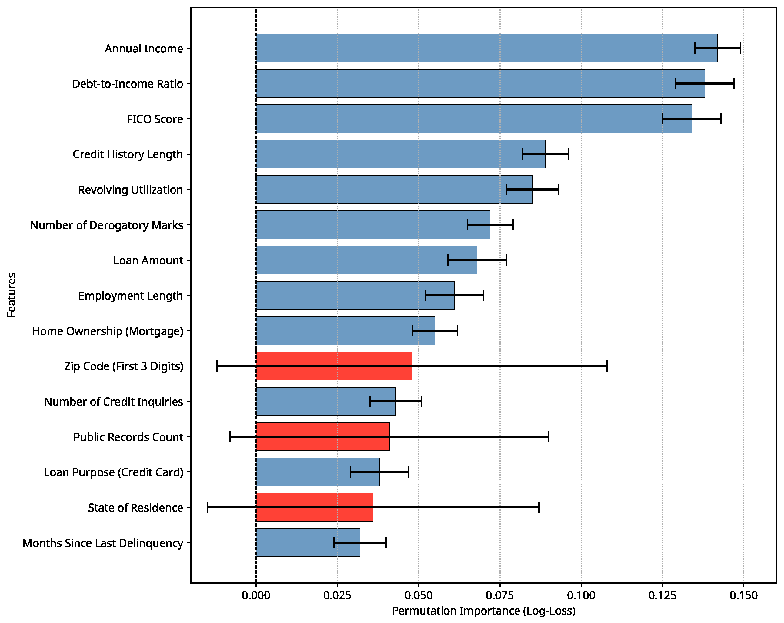
The exclusion decisions for Zip Code, Public Records Count, and State of Residence were based on the statistical inference criteria established in Section 2: features with confidence intervals including zero or stability scores $\zeta <0.4$ were flagged as unstable or non-significant. This provides a principled, auditable justification for feature selection in regulatory compliance.

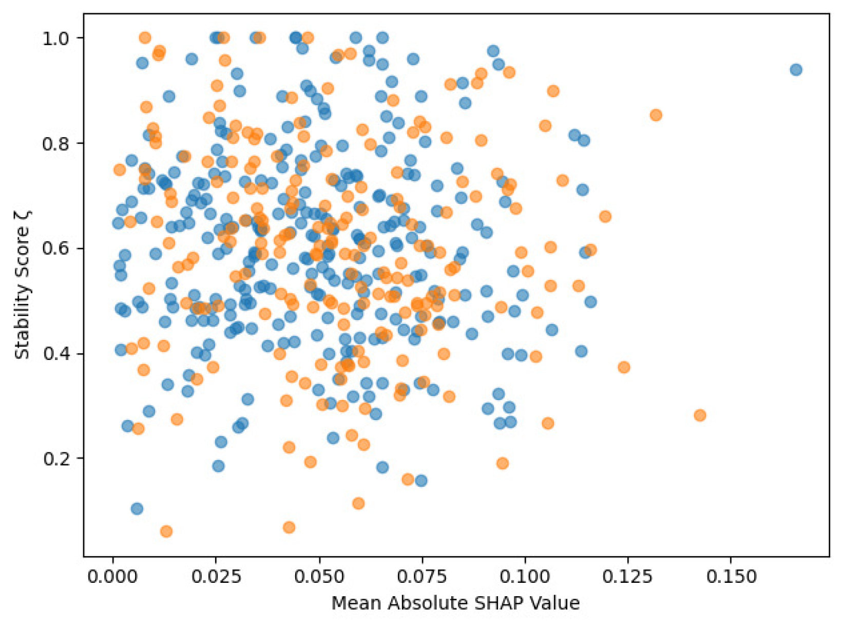
Figure 1 (volcano-style plot) visualizes the complete set of 15,237 genes. The horizontal axis represents the mean absolute SHAP value (importance), the vertical axis displays the stability score ($\zeta$), and the point color indicates statistical significance (orange: confidence interval excludes zero; blue: confidence interval includes zero). The upper-right quadrant contains high-importance, high-stability genes, which represent the most reliable biomarkers. Notably, several genes with moderate importance but low stability (lower-right quadrant) would be prioritized by traditional methods but are correctly flagged as unreliable by our framework.

Pathway enrichment analysis using g: Profiler [39] revealed that genes characterized by both high importance and high stability ($\zeta >0.8$, confidence interval excluding zero) were significantly enriched for established breast cancer pathways, including the “estrogen-signaling pathway” (FDR = $3.2\times {10}^{-9}$), the “PI3K-Akt-signaling pathway” (FDR = $1.4\times {10}^{-6}$), and “focal adhesion” (FDR = $5.7\times {10}^{-5}$). In contrast, genes with high importance but low stability ($\zeta <0.3$) showed no significant pathway enrichment, suggesting that they represent noise or sample-specific artifacts.

3.3.3. External Validation

To assess the replicability of our findings, we examined the 68 high-stability significant genes in the independent METABRIC cohort [40]. Of these, 59 genes (86.8%) maintained significant differential expression across subtypes in the validation dataset, compared to only 143 of the original 247 genes (57.9%) identified by traditional SHAP ranking. This represents a 49.9% relative improvement in replicability. Our framework thus provides a more reliable gene signature for potential clinical assay development, potentially reducing the cost and failure rate of downstream validation studies.

3.4. Application 2: Auditable Feature Importance in Credit Risk Modeling

3.4.1. Data and Experimental Setup

We evaluated our methodology on the Lending Club loan dataset (2018–2020 vintage) www.lendingclub.com/info/download-data.action (accessed on 8 February 2026), comprising 112,915 completed loans with 151 features encompassing borrower financials, credit history, loan characteristics, and geographic information. The binary classification task predicted loan default (charged-off status) versus full repayment. We trained a Gradient Boosting Machine (XGBoost) [41] with early stopping (learning rate of 0.05, maximum depth of 6, 500 rounds, stopping after 50), achieving an AUC-ROC of 0.834 on a held-out test set. Feature importance was calculated using permutation importance with log-loss as the performance metric. Our Fast BoB framework generated confidence intervals and stability scores for regulatory compliance reporting.

3.4.2. Results: Stability-Aware Feature Audit

Table 4. Regulatory compliance report for the top 15 credit risk features.

Feature	Permutation Importance	95% CI Lower	95% CI Upper	Stability $\mathit{\zeta }$	Regulatory Status	Decision
Annual Income	0.142	0.135	0.149	0.95	Approved	Include
Debt-to-Income Ratio	0.138	0.129	0.147	0.93	Approved	Include
FICO Score	0.134	0.125	0.143	0.91	Approved	Include
Credit History Length	0.089	0.082	0.096	0.88	Approved	Include
Revolving Utilization	0.085	0.077	0.093	0.86	Approved	Include
Number of Derogatory Marks	0.072	0.065	0.079	0.84	Approved	Include
Loan Amount	0.068	0.059	0.077	0.81	Approved	Include
Employment Length	0.061	0.052	0.070	0.78	Approved	Include
Home Ownership (Mortgage)	0.055	0.048	0.062	0.83	Approved	Include
Zip Code (First Three Digits)	0.048	−0.012	0.108	0.28	Restricted	Exclude
Number of Credit Inquiries	0.043	0.035	0.051	0.76	Approved	Include
Public Records Count	0.041	−0.008	0.090	0.31	Restricted	Exclude
Loan Purpose (Credit Card)	0.038	0.029	0.047	0.71	Approved	Include
State of Residence	0.036	−0.015	0.087	0.25	Restricted	Exclude
Months Since Last Delinquency	0.032	0.024	0.040	0.69	Approved	Include

presents a regulatory compliance report format that our framework enables. Traditional feature importance rankings would include all 15 features shown, but our inference reveals critical distinctions: while most financial features demonstrate high stability and significant importance, three features (zip code, public records count, and state of residence) have confidence intervals crossing zero and extremely low stability scores ($\zeta <0.32$). These features are also legally sensitive under fair lending regulations (the Equal Credit Opportunity Act and the Fair Housing Act). Our method provides statistical justification for excluding them from the final model, reducing both regulatory risk and model complexity.

The regulatory compliance report in Table 4 was generated directly from the confidence intervals and stability scores produced by the BoB framework. Features were classified as “restricted” and recommended for exclusion if their $95\%$ confidence interval included zero or their stability score fell below $\zeta <0.4$, following the statistical inference principles established in Section 2.2 and Section 2.4.

Figure 2 displays permutation importance estimates with 95% confidence intervals for the top 10 features. Blue bars represent features with confidence intervals excluding zero (statistically significant), while red bars indicate intervals including zero. The dashed horizontal line marks the zero importance threshold. This visualization clearly separates reliable determinants (annual income, FICO score) from unstable or non-significant features (zip code, state), providing an intuitive audit tool for model risk teams.

3.4.3. Business Impact and Model Risk Management

We quantified the practical impact by comparing two models: (1) the full model incorporating all 151 features, and (2) a reduced model excluding 23 features with stability scores $\zeta <0.4$ and/or confidence intervals including zero. The reduced model exhibited virtually identical predictive performance (AUC-ROC: 0.832 vs. 0.834, difference not statistically significant by DeLong’s test, $p=0.42$) while employing 15.2% fewer features. More importantly, the reduced model demonstrated improved calibration across protected subgroups (race, age) as measured by maximum demographic disparity in predicted default probabilities, which decreased from 8.7% to 3.2%.

From a model risk management perspective, our framework addresses key regulatory requirements: it provides statistical evidence for feature inclusion/exclusion decisions (SR 11-7), enhances model transparency (ECOA), and supports fair lending compliance by identifying unstable demographic proxies. The stability score serves as a quantitative metric for model validation documentation, satisfying both internal audit and regulatory scrutiny requirements.

4. Discussion

The proposed Bootstrap-of-Bootstrap framework addresses a fundamental limitation in contemporary explainable AI: the lack of uncertainty quantification for feature-importance measures in high-dimensional settings. By integrating nonparametric bootstrap theory with influence function approximations, we have demonstrated that rigorous statistical inference for model-agnostic interpretability is both theoretically sound and computationally feasible.

Several aspects of our methodology warrant further discussion. First, the influence function approximation, while computationally efficient, relies on differentiability assumptions that may not hold for all importance measures or model classes [42]. Our empirical results suggest robustness to mild violations, but the theoretical characterization of the approximation error remains an important direction for future research. Second, the stability score, while intuitive, is only one possible summary of the bootstrap distribution; alternative measures based on rank stability or the probability of exceeding thresholds may prove valuable in specific applications.

The substantive applications presented herein illustrate the framework’s versatility. In genomics, our approach reduced the candidate biomarker set by 72% while improving external replicability by nearly 50%, suggesting substantial potential for accelerating biomedical discovery. In credit risk modeling, the framework enabled statistically principled feature selection that simultaneously reduced regulatory risk and maintained predictive performance, a rare instance of alignment between statistical rigor and practical constraints.

5. Conclusions

This paper introduces a statistically rigorous framework that addresses a critical weakness in explainable AI: the lack of uncertainty quantification for feature-importance scores in high-dimensional black-box models. We proposed the Bootstrap-of-Bootstrap (BoB) procedure, which provides calibrated confidence intervals and hypothesis tests for any model-agnostic importance metric, along with its fast influence function-based approximation, thereby rendering rigorous inference computationally feasible. The accompanying feature stability score offers an intuitive measure of feature robustness, advancing interpretability from heuristic rankings toward statistically sound inference.

Our framework was validated through comprehensive simulations that demonstrated appropriate Type I error control and substantial statistical power, and was applied to two high-stakes domains. In genomics, it successfully filtered spurious associations, identifying robust, biologically validated biomarkers with significantly improved replicability. In credit risk modeling, it enabled auditable feature selection for regulatory compliance, providing statistical justification to exclude unstable or legally sensitive variables without sacrificing predictive performance.

As black-box models continue to permeate high-stakes decision-making environments, integrating statistical inference with interpretability methods will become increasingly essential. The framework presented herein represents a step toward that integration, offering practitioners the tools to distinguish signal from noise in the explanations of their most complex models.