Improved Confidence Interval Estimation for Zero-Inflated Count Data Using Transformed Two-Part Bootstrap

Abstract

This study proposes a transformed two-part bootstrap confidence interval (TTB-CI) for zero-inflated count data. The method combines a standard zero-inflated mixture formulation, parametric bootstrap, and monotone transformations to improve inference for practically meaningful estimands, including the marginal mean, zero probability, and positive-part mean. Simulation studies under zero-inflated Poisson (ZIP) and zero-inflated negative binomial (ZINB) data-generating processes show that the proposed method maintains nominal or near-nominal coverage while reducing interval width, particularly for the positive-part mean. Compared with conventional Poisson- and negative binomial-based confidence intervals, the proposed TTB-CI provides a more favorable coverage and width tradeoff and yields more informative intervals for positive count inference. These results indicate that the proposed method offers a practical and efficient confidence interval framework for zero-inflated count data.

1. Introduction

Count data with an excess number of zeros arise frequently in many scientific and applied fields, including epidemiology, health economics, insurance analytics, transportation studies, and text or event-count analysis [1,2,3,4,5,6,7]. In such data, the observed proportion of zeros often exceeds what standard count models, such as the Poisson or negative binomial model, can adequately explain [1,2,3]. This phenomenon is commonly referred to as zero inflation and has motivated the use of zero-inflated Poisson (ZIP) and zero-inflated negative binomial (ZINB) models [1,2,3,8]. Zero-inflated models represent the data-generating process as a mixture of a structural-zero component and an ordinary count component [1,2,3]. Thus, zero observations may arise either from a structural-zero mechanism or from the count distribution itself. This differs from hurdle models, where all zero observations are generated by a separate zero process and the positive-count component is zero-truncated [1,2,3,7]. In this study, we focus on standard zero-inflated models because they are appropriate when both structural zeros and sampling zeros are plausible [1,2,3]. While model fitting and point estimation for zero-inflated data have been widely studied, confidence interval estimation for interpretable nonlinear estimands, such as the marginal mean, zero probability, and positive-part mean, remains less developed [5,6,9,10,11,12,13,14,15,16,17]. This motivates the transformed two-part bootstrap confidence interval proposed in this study.

From a practical perspective, reliable confidence intervals for zero-inflated data are important because many applied studies require uncertainty quantification rather than point estimation alone. For example, in epidemiology and health care studies, the frequency of zero events may correspond to individuals or regions with no observed disease cases, while the positive counts may represent outbreak intensity or treatment burden [1,2]. In text mining and count events analysis, many keywords or events may be absent in most observations, while non-zero counts carry important information about activity intensity [4,6]. Therefore, confidence intervals that maintain nominal coverage while avoiding unnecessarily wide intervals are practically important for interpretable and reliable decision making [5,9].

A particularly challenging issue arises from the fact that, in zero-inflated data, the majority of observations may be equal to zero. As a result, confidence intervals constructed using standard Poisson or negative binomial assumptions tend to concentrate excessively near zero or exhibit strong conservatism [1,14,15,16,17]. This problem is especially pronounced for the positive-part mean, where removing zeros can induce severe skewness and instability in the sampling distribution. Consequently, conventional confidence intervals may exhibit either under-coverage or overly wide intervals, limiting their practical usefulness. Negative binomial models are frequently adopted to address overdispersion in count data [2,3]. However, even when combined with zero-inflation, negative binomial-based confidence intervals typically target the conditional mean of the count component, rather than the marginal or positive-part mean [18,19,20,21]. This mismatch between the estimate of interest and the parameter being inferred can further degrade interval performance, particularly when the proportion of structural zeros is large. Moreover, analytic confidence intervals for nonlinear functionals of zero-inflated models are generally unavailable in closed form, making inference even more challenging. Bootstrap-based methods offer a natural alternative for interval estimation in complex models [22,23,24,25,26]. By approximating the sampling distribution of an estimator through resampling, bootstrap techniques can accommodate nonlinearity, skewness, and complex dependence structures. Nevertheless, naïve bootstrap confidence intervals applied directly to zero-inflated data often remain unstable due to boundary effects and highly skewed distributions, especially when the target parameter is constrained or involves ratios of random quantities.

Recent studies further demonstrate that zero-inflated modeling remains an active and evolving research area. In healthcare applications, zero-inflated count regression models have been used to address excess zeros and stay data with outliers, highlighting the practical importance of robust zero-inflated inference [27]. Recent work on ZINB models with incomplete covariates has also developed inverse probability weighting and semiparametric estimation procedures, emphasizing that zero inflation and missingness can jointly affect parameter estimation [28]. In addition, recent distributional extensions, such as arbitrarily inflated negative binomial regression models, generalize conventional zero-inflated models by allowing excess probability mass at multiple count values rather than only at zero [29]. Other studies have compared traditional ZIP and ZINB models with machine learning methods for zero-inflated and overdispersed ecological count data [30]. These developments show that recent research has mainly focused on model fitting, prediction, missing data, and distributional flexibility, whereas reliable confidence interval estimation for nonlinear zero-inflated estimands remains comparatively less developed.

The remainder of this paper is organized as follows. Section 2 reviews existing interval estimation methods for Poisson and negative binomial models and discusses their limitations in zero-inflated settings. Section 3 introduces the proposed TTB-CI method, including the model formulation, transformation, bootstrap procedure, and confidence interval construction. Section 4 presents the simulation studies and real data application used to evaluate the proposed method against conventional approaches. Section 5 discusses the motivations, contributions, and limitations of our research. Finally, Section 6 concludes the paper by summarizing the main findings, describing the methods and results of our study, and suggesting directions for future research.

2. Existing Interval Estimation and Limitations

Conventional confidence intervals for count data are commonly developed under standard Poisson or negative binomial assumptions. For Poisson count data, an exact confidence interval for the mean parameter can be obtained from the total count $S={\displaystyle {\sum }_{i=1}^n}{Y}_i$. A commonly used 100(1 − α)% exact confidence interval is written as follows [1,31,32,33,34].

$${CI}_{pois}\left(\lambda \right)=\left({\displaystyle \frac{1}{2n}}{\chi }_{2S,\alpha /2}^2, {\displaystyle \frac{1}{2n}}{\chi }_{2\left(S+1\right),(1-\alpha /2)}^2\right)$$

(1)

In Equation (1), ${\chi }_{\nu ,p}^2$ denotes the p-th quantile of the chi-square distribution with ν degrees of freedom. When S = 0, the lower confidence limit is defined as zero. For overdispersed count data, negative binomial models are often used instead of Poisson models. Since a simple exact confidence interval is generally unavailable for the negative binomial mean, likelihood-based or asymptotic confidence intervals are commonly used [1,2,3,18,19,20,21,35,36]. A profile likelihood confidence interval for the mean parameter $\mu$ can be expressed as follows.

$${CI}_{NB}\left(\mu \right)=\left(\mu :2\left[lp\left(\widehat{\mu }\right)-lp\left(\mu \right)\right]\le {\chi }_{1,(1-\alpha )}^2\right)$$

(2)

In Equation (2), $lp\left(\mu \right)$ is the profile log-likelihood for $\mu$, and $\widehat{\mu }$ is the maximum likelihood estimate. Although these conventional intervals are well established, they are primarily designed for data generated from a single count process. In zero-inflated count data, however, observed zeros may arise from both a structural-zero component and an ordinary count-generating component. Therefore, a confidence interval constructed using all observations may be overly influenced by excessive zeros and may concentrate near zero. Conversely, a confidence interval constructed after removing zeros may ignore the zero-generating mechanism and may fail to reflect the uncertainty induced by the two-part structure [5,9,11,12,13,14,15,16,17]. This issue is closely related to the distinction between zero-inflated models and hurdle models. In zero-inflated models, zero observations may arise from both the structural-zero component and the ordinary count component. For example, in road crash count data, a road segment may have zero crashes because it is structurally low-risk, or because no crash occurs by chance during the observation period despite being exposed to traffic. In contrast, hurdle models assume that all zero observations are generated by a separate zero process and that the positive-count component is zero-truncated [1,2,3,7]. Consequently, standard Poisson or negative binomial confidence intervals do not directly address nonlinear zero-inflated estimands such as the marginal mean, zero probability, and positive-part mean. These quantities depend jointly on the zero-generating and count-generating components, and their sampling distributions may be affected by skewness, boundary constraints, and the large point mass at zero. This motivates the transformed two-part bootstrap confidence interval proposed in Section 3.

3. Proposed Method

In this paper, we propose a TTB-CI to overcome the problem of existing methods, which produce widely distributed confidence intervals around zero for zero-inflated count data. The proposed method is based on bootstrap inference, which provides a nonparametric approximation to the sampling distribution of complex estimators. Under standard regularity conditions, the bootstrap distribution consistently approximates the sampling distribution of the estimator, ensuring asymptotic validity of the resulting confidence intervals. Combining a two-part model representation, parametric bootstrap, and scale transformation, the proposed method aims to simultaneously achieve stable coverage and efficient interval width even in the presence of zero inflation and overdispersion. The proposed TTB-CI is constructed under a standard zero-inflated mixture formulation, rather than a hurdle formulation. In this formulation, the count component is an ordinary Poisson or negative binomial distribution and is not zero-truncated.

$$Y_i=\left\{\begin{array}{cc}0& ,Z_i=1\\ Y_i^{*}& ,Z_i=0\end{array}\right.\hspace{1em}{Y}_i^{*}~f\left({\theta }_i\right), Z_i~Bernoulli\left({\pi }_i\right)$$

(3)

Since $Y_i^{*}$ follows an ordinary count distribution, it may also take the value zero in Equation (3). Therefore, the observed zero probability is not simply ${\pi }_i$, but is given by

$$\mathrm{P}\left(Y_i=0\right)={\pi }_i+\left(1-{\pi }_i\right)f\left(0;{\theta }_i\right)$$

(4)

In Equation (4), ${\pi }_i=P\left(Z_i=1\right)$ is the probability of structural zero. It is important to note that the count component is not zero-truncated. Therefore, zero outcomes may arise from both the structural zero component and the count distribution. This distinguishes the zero-inflated model from hurdle-type models, in which the count component generates only strictly positive values. Our method is based on a working zero-inflated model, which assumes conditional independence between the zero-generating process and the count-generating process given the observed covariates. We assume two working models for the count state, Poisson and negative binomial working models.

Table 1. Standard zero-inflated model structure with Poisson and negative binomial count components.

Component	Latent State	Observed Outcome	Distribution
Structural zero	$Z_i=1$	$Y_i=0$	Point mass at zero
Count component	$Z_i=0$	$Y_i~f\left(y;{\theta }_i\right)$	Poisson or negative binomial

shows the parameters, means, and variances of the two models [2].

It is important to note that the count component is not zero-truncated. Therefore, zero outcomes may arise from both the structural component and the count distribution. This distinguishes the zero-inflated model from hurdle-type models, where the count component generates only strictly positive values. For the confidence intervals of the Poisson and negative binomial distributions, we consider the following generalized linear model (GLM) for each observation i [1,2].

$$log\left({\mu }_i\right)=x_i^T\beta , logit\left({\pi }_i\right)=x_i^T\tau$$

(5)

In Equation (5), $x_i=\left(1,X_{i1},X_{i2},\dots ,X_{ip}\right)$ is a covariate vector. In our research, we obtain three values: marginal mean, zero probability, and positive-part mean. First, the marginal mean is calculated as in Equation (6) [1,2].

$$E\left(Y\right)={\displaystyle \frac{1}{n}}{\displaystyle {\sum }_{i=1}^n}\left(1-{\pi }_i\right){\mu }_i$$

(6)

Next, we compute the probability $P_0=P\left(Y=0\right)$ for zero. The proposed model computes $P_0$ for two cases, Poisson and negative binomial. In the ZIP model based on the Poisson probability distribution, $P_0$ is computed as Equation (7).

$$P_0={\displaystyle \frac{1}{n}}{\displaystyle {\sum }_{i=1}^n}\left({\pi }_i+\left(1-{\pi }_i\right)e^{-{\mu }_i}\right)$$

(7)

The following Equation (8) represents the formula for calculating $P_0$ in the ZINB model based on the negative binomial probability distribution.

$$P_0={\displaystyle \frac{1}{n}}{\displaystyle {\sum }_{i=1}^n}\left({\pi }_i+\left(1-{\pi }_i\right){\left({\displaystyle \frac{\theta }{\theta +{\mu }_i}}\right)}^{\theta }\right)$$

(8)

We obtain the positive-part mean using the following Equation (9).

$$E\left(Y|Y>0\right)={\displaystyle \frac{E\left(Y\right)}{1-P_0}}$$

(9)

The conventional Poisson or negative binomial-based confidence intervals mainly provide inference for $\mu$ itself, but in the zero-inflated setting, marginal or conditional estimate mismatch occurs. The analytic confidence intervals for the above estimates are difficult to derive in closed form. Therefore, this study attempts to address this difficulty by using an approach based on parametric bootstrapping. Our parametric bootstrap under a two-part working model consists of three steps [23]. In the first step, we perform model fitting. Using the observed data $D=\left(Y_i,x_i\right),i=\mathrm{1,2},\dots ,n$, we fit the ZIP and ZINB working models to estimate $\widehat{\beta }$, $\widehat{\tau }$ and $\widehat{\theta }$. In the second step, we perform bootstrap resampling $b=\mathrm{1,2},\dots ,B$ times repeatedly. We extract $Z_i$ from $Z_i^{\left(b\right)}~Bernoulli\left({\widehat{\pi }}_i\right)$ and generate $Y_i^{\left(b\right)}$ from $Poisson\left({\widehat{\mu }}_i\right)$ or $NB\left({\widehat{\mu }}_i,\widehat{\theta }\right)$ if $Z_i^{\left(b\right)}=0$. Through this, we build a bootstrap dataset $D^{\left(b\right)}$. In the third step, we refit the same working model for each $D^{\left(b\right)}$ and estimate ${\widehat{T}}^{\left(b\right)}=\left({\widehat{P}}_0^{\left(b\right)},\widehat{E}{\left(Y|Y>0\right)}^{\left(b\right)}\right)$. Because bootstrap distributions are often skewed or bounded, percentile confidence intervals at the original scale may have unstable coverage. To compensate for this, this study uses transformed percentile confidence intervals. In this paper, we use two transformations. First, the logit function for $P_0$ as shown in Equation (10):

$$g_1\left(P_0\right)=logit\left(P_0\right)=log\left({\displaystyle \frac{P_0}{1-P_0}}\right)$$

(10)

The transformation functions are introduced to map the parameters to an unconstrained domain. The logit transformation is used for the zero probability, while the logarithmic transformation is applied to the positive-part mean to ensure positivity and reduce skewness. This transformation alleviates the boundary issue by mapping the interval values of $\left(\mathrm{0,1}\right)$ to $\left(-\infty ,\infty \right)$ and enables transformed confidence intervals. The following Equation (11) is a transformation for $E\left(Y|Y>0\right)>0$.

$$g_2\left(E\left(Y|Y>0\right)\right)=log\left(E\left(Y|Y>0\right)\right)$$

(11)

Based on this transformation, we construct the following confidence interval for bootstrap replicates $g\left(T^{\left(b\right)}\right)$.

$$\left(g^{-1}\left(q_{\alpha /2}\right),g^{-1}\left(q_{(1-\alpha /2)}\right)\right)$$

(12)

In Equation (12), $q_{\nu }$ denotes the empirical $\nu$ quantile. To ensure coverage of the confidence interval, the following inflation adjustment is applied to the transformed scale.

$$g^{*}\left(T^{\left(b\right)}\right)=\tilde{g}+\mathsf{\kappa }\left(g\left(T^{\left(b\right)}\right)-\tilde{g}\right)$$

(13)

In Equation (13), $\tilde{g}$ is the median of bootstrap replicates $\mathsf{\kappa }>1$ is an inflation factor that controls the spread of the bootstrap distribution on the transformed scale. It is introduced to adjust for finite-sample bias and to improve coverage accuracy. The calibration of Equation (13) secures nominal coverage by stabilizing the tail behavior of the bootstrap distribution without artificially expanding the variance. The TTB-CI proposed in this paper has four key features. First, it explicitly reflects zero inflation through two-part decomposition. Second, it enables inference for estimates through parametric bootstrap. Furthermore, it mitigates the skewness and boundary problems through transformation and ensures coverage stability even under misspecification through calibration step. The following Algorithm 1 demonstrates a procedure for constructing stable confidence intervals for zero probability and positive-part mean by combining a two-part working model, parametric bootstrap, and scale transformation for zero-inflated count data.

Algorithm 1 Transformed Two-Part Bootstrap Confidence Interval (TTB-CI)

Input: $\hspace{1em}D=\left(Y_i,x_i\right)$: observed data $\hspace{1em}M\in \left(ZIP, ZINB\right)$: working model  B: number of bootstrap replications $\hspace{1em}1-\mathsf{\alpha }$: confidence level  $\mathsf{\kappa }$: inflation factor that controls dispersion of bootstrap distribution on transformed scale

Output:  Confidence intervals for    $\mathrm{Zero} \mathrm{probability} P_0=P\left(Y=0\right)$    $\mathrm{Positive}\text{-}\mathrm{part} \mathrm{mean} E\left(Y|Y>0\right)$ Step1: Two-part model fitting  $\mathrm{Fit} \mathrm{two}\text{-}\mathrm{part} \mathrm{regression} \mathrm{model} \mathrm{to} D, log\left({\mu }_i\right)=x_i^T\beta$$, logit\left({\pi }_i\right)=x_i^T\tau$    ${\pi }_i$$: \mathrm{structural} \mathrm{zero} \mathrm{probability}, {\mu }_i$: mean of count state  $\mathrm{If} M=ZIP$$: Y_i~Poisson\left({\mu }_i\right)$  $\mathrm{If} M=ZINB$$: Y_i~NB\left({\mu }_i,\theta \right)$  $\mathrm{Obtain} \mathrm{parameter} \mathrm{estimates} \left(\widehat{\beta },\widehat{\tau }\right)$$\mathrm{and} \mathrm{if} \mathrm{applicable} \widehat{\theta }$ Step2: Target estimate computation  Compute plug-in estimators using fitted model    $\mathrm{Marginal} \mathrm{mean}: E\left(Y\right)={\displaystyle \frac{1}{n}}{\displaystyle {\sum }_{i=1}^n}\left(1-{\pi }_i\right){\mu }_i$    Zero probability      $\mathrm{Poisson}: P_0={\displaystyle \frac{1}{n}}{\displaystyle {\sum }_{i=1}^n}\left({\pi }_i+\left(1-{\pi }_i\right)e^{-{\mu }_i}\right)$,      $\mathrm{Negative} \mathrm{binomial}: P_0={\displaystyle \frac{1}{n}}{\displaystyle {\sum }_{i=1}^n}\left({\pi }_i+\left(1-{\pi }_i\right){\left({\displaystyle \frac{\theta }{\theta +{\mu }_i}}\right)}^{\theta }\right)$    $\mathrm{Positive}\text{-}\mathrm{part} \mathrm{mean}: E\left(Y|Y>0\right)={\displaystyle \frac{E\left(Y\right)}{1-P_0}}$ Step3: Parametric bootstrap sampling  $\mathrm{Generate} \mathrm{latent} \mathrm{indicator}, Z_i^{\left(b\right)}~Bernoulli\left({\widehat{\pi }}_i\right)$  $\mathrm{If} Z_i^{\left(b\right)}=1$$, \mathrm{set} Y_i^{\left(b\right)}=0$  $\mathrm{If} Z_i^{\left(b\right)}=0$$, \mathrm{generate} Y_i^{\left(b\right)}~Poisson\left({\widehat{\mu }}_i\right)$$\mathrm{or} Y_i^{\left(b\right)}~NB\left({\widehat{\mu }}_i,\widehat{\theta }\right)$  $\mathrm{Construct} \mathrm{bootstrap} \mathrm{dataset} D^{\left(b\right)}=\left(Y_i^{\left(b\right)},x_i\right)$  $\mathrm{Refit} \mathrm{same} \mathrm{two}\text{-}\mathrm{part} \mathrm{model} \mathrm{to} D^{\left(b\right)}$  $\mathrm{Compute} {\widehat{T}}^{\left(b\right)}=\left({\widehat{P}}_o^{\left(b\right)},\widehat{E}{\left(Y|Y>0\right)}^{\left(b\right)}\right)$ Step4: Scale transformation  Apply monotone transformations to stabilize skewness and boundary effects:    $g_1\left(P_0\right)=logit\left(P_0\right)=log$$, g_2\left(E\left(Y|Y>0\right)\right)=log\left(E\left(Y|Y>0\right)\right)$  $\mathrm{Let}: T_g^{\left(b\right)}=\left(g_1\left({\widehat{P}}_o^{\left(b\right)}\right),g_2\left(\widehat{E}{\left(Y|Y>0\right)}^{\left(b\right)}\right)\right)=\left(log\left({\displaystyle \frac{{\widehat{P}}_o^{\left(b\right)}}{1-{\widehat{P}}_o^{\left(b\right)}}}\right),log\left(\widehat{E}{\left(Y|Y>0\right)}^{\left(b\right)}\right)\right)$ Step5: Inflation adjustment (coverage calibration)  $\mathrm{Let} \tilde{g}$ denote the componentwise median of the transformed bootstrap replicates  Apply inflation on the transformed scale:    $T_g^{\left(b\right)*}=\tilde{g}+\mathsf{\kappa }\left(T_g^{\left(b\right)}-\tilde{g}\right)$  Where κ > 1 is an inflation factor controlling the spread of the bootstrap distribution. Step6: Transformed percentile confidence intervals  $\mathrm{For} \mathrm{each} \mathrm{component} (\mathsf{\kappa }=\mathrm{1,2}$$) \mathrm{compute} \left(q_{\alpha /2}\left(T_{g,k}^{*\left(b\right)}\right),q_{(1-\alpha /2)}\left(T_{g,k}^{*\left(b\right)}\right)\right)$ Step7: Back transformation  Obtain final confidence intervals on original scale    ${CI}_{1-\alpha }\left(P_0\right)={logit}^{-1}\left({CI}_{1-\alpha }\left(g_1\right)\right)$    ${CI}_{1-\alpha }\left(E\left(Y|Y>0\right)\right)=exp\left({CI}_{1-\alpha }\left(g_2\right)\right)$

In this study, the inflation factor κ is selected from a predefined grid using a pilot simulation calibration procedure. The value of $\mathsf{\kappa }$ is chosen to achieve empirical coverage close to the nominal level while maintaining a minimal interval width. In this study, κ was selected to satisfy the nominal 95% coverage condition. In Algorithm 1, we summarize the proposed method procedurally described in this section. Our proposed TTB-CI accommodates both Poisson and negative binomial count components within a unified framework, and the inflation step enhances finite sample coverage robustness under model misspecification. In the following section, we conduct experiments to compare the performance of the proposed method on ZIP and ZINB with traditional methods. Finally, we show the following proposition.

Proposition 1.

Under standard regularity conditions and a correctly specified zero-inflated model, the proposed transformed bootstrap confidence interval is asymptotically valid in the sense that its coverage probability converges to the nominal confidence level as the sample size tends to infinity in Equation (14).

$$\underset{n\to \infty }{\lim }P\left(T\in {CI}_{TTB,n}\left(1-\alpha \right)\right)=1-\alpha$$

(14)

In Equation (14), ${CI}_{TTB,n}\left(1-\alpha \right)$ denotes the $100\left(1-\alpha \right)\%$ confidence interval set constructed by the proposed TTB-CI method from a sample of size n.

$${CI}_{TTB,n}\left(1-\alpha \right)=\left(L_{TTB,n}, U_{TTB,n}\right)$$

(15)

In Equation (15), $L_{TTB,n}$ and $U_{TTB,n}$ are the lower and upper confidence limits obtained from the transformed bootstrap quantiles. For multiple target estimands, the confidence interval is interpreted componentwise. The conditional independence assumption means that, after conditioning on the observed covariates, the structural zero mechanism and the count-generating mechanism are assumed to be independent. For example, in healthcare utilization data, an unobserved health severity factor may affect both whether an individual has any outpatient visit and how many visits occur among individuals with positive visits. If this latent factor is not included as a covariate, the zero-generating process and the count-generating process may be correlated through their unobserved errors. In this case, the estimated zero probability and count mean may be biased, and the resulting confidence intervals may not achieve exact nominal coverage. The bootstrap procedure would then approximate the sampling distribution under the assumed working model rather than the true data-generating process. Therefore, the proposed TTB-CI should be interpreted as a model-based inference procedure whose validity depends on the adequacy of the working zero-inflated model and its conditional independence assumption.

4. Experimental Results of Simulation and Real Data

To demonstrate the validity of the proposed method, we analyzed two types of simulation data using R version 4.5.0 (R Foundation for Statistical Computing, Vienna, Austria) [37]. First, we generated simulation data from the zero-inflated negative binomial distribution. In our experiments, we compared the proposed models with general ZIP and ZINB models by the width of confidence interval and the coverage. To evaluate the performance of confidence intervals for zero-inflated count data, this study uses a two-part data-generating mechanism that separates structural zeros from count states. The count state distribution is set to Poisson and negative binomials, and the sensitivity of confidence intervals to distributional assumptions is also evaluated. We generated two zero-inflated count datasets as follows. In both simulation settings, the covariates were generated independently from a standard normal distribution. Specifically, for each observation $i=1,2,\dots ,n$ and each covariate $j=1,2,\dots ,p$ we generated $X_{ij}~N\left(\mathrm{0,1}\right), i=\mathrm{1,2},\dots ,n , j=\mathrm{1,2},\dots ,p$. Equivalently, the covariate vector was generated as $X_i={\left(X_{i1},X_{i2},\dots ,X_{ip}\right)}^T~N\left(0,I_p\right)$.

In this study, we set $\mathrm{n}=5000$ and $p=5$. The same covariate-generation mechanism was used for both the ZIP and ZINB simulation studies. The covariates themselves were not zero-inflated; zero inflation was introduced only in the response variable through the structural-zero mechanism.

In the simulation study, we set the sample size to n = 5000 and the number of covariates to p = 5. The sample size was chosen to represent a moderately large zero-inflated count data setting in which bootstrap-based confidence intervals can be evaluated stably while maintaining feasible computational time. The number of covariates was fixed at five to represent a multivariable regression setting while avoiding unnecessary model complexity. The same values of n and p were used for both the ZIP and ZINB simulations so that the effect of the count distribution could be compared under a common design.

The sample size directly affects interval estimation. As n increases, the bootstrap distribution becomes more stable and the interval width generally decreases at the usual ${\displaystyle \frac{1}{\sqrt{n}}}$ rate. In contrast, when n is small, the effective number of positive observations may be limited in zero-inflated data, resulting in wider intervals and less stable coverage, particularly for E(Y∣Y > 0). Therefore, the simulation results should be interpreted as representing a moderately large sample setting, and further sensitivity studies over different sample sizes and numbers of covariates remain an important direction for future work.

In Algorithm 2, the Poisson setting corresponds to ZIP data-generating process, while the negative binomial setting induces the ZINB process with overdispersion. By considering both settings within a unified simulation framework, we assess the robustness of the proposed confidence interval method to distributional assumptions in the count component. In the computational implementation used for our simulation results, the inflation factor was set to ${\kappa }_{ZIP}=1.00$ for the ZIP simulation and ${\kappa }_{ZINB}=1.00$ for the ZINB simulation. Thus, no additional inflation beyond the transformed bootstrap distribution was applied. 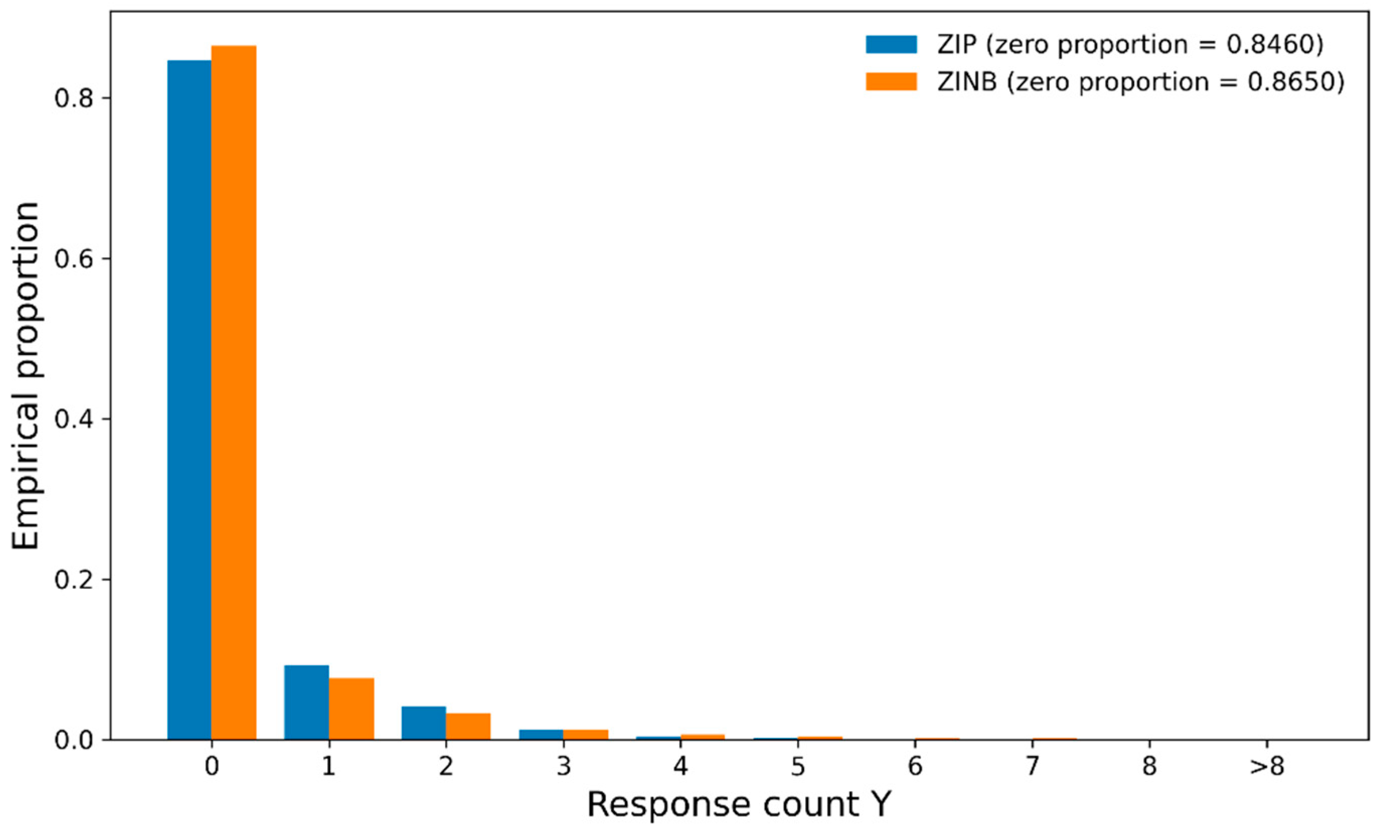We represent Figure 1 for the distribution of simulated response variables under the ZIP and ZINB data-generating processes as follows. The high frequency at zero indicates the zero-inflated structure of the generated count data.

Algorithm 2 Simulation of zero-inflated count data from Poisson and negative binomial

Input:  n: sample size  p: number of predictors  ${\beta }_0,{\beta }_1,\dots ,{\beta }_p$: regression coefficients of count part  ${\tau }_0,{\tau }_1,\dots ,{\tau }_p$: regression coefficients of zero-inflated part  ${\mu }_{max}$: maximum cap  $D: \mathrm{distribution} \mathrm{indicator}, D\in \left\{Poisson, Negative binomial\right\}$  $\mathsf{\gamma }$: dispersion parameter used only when D is negative binomial

Output:  $\left(Y_i,X_{i1},X_{i2},\dots ,X_{ip}\right)$$, i=\mathrm{1,2},\dots ,n$: simulated data Step1: Generate predictors  $\mathrm{For} \mathrm{each} \mathrm{observation} i=\mathrm{1,2},\dots ,n$$\mathrm{and} \mathrm{predictor} j=\mathrm{1,2},\dots ,p$  $\mathrm{Generating} X_{ij}~N\left(\mathrm{0,1}\right)$$, \mathrm{equivalently} X_i={\left(X_{i1},X_{i2},\dots ,X_{ip}\right)}^T~N\left(0,I_p\right)$  $\mathrm{In} \mathrm{this} \mathrm{simulation} \mathrm{study}, p=5$, and the covariates are generated independently Step2: Specify count component  Compute linear predictor and mean intensity using log-link function  ${\eta }_i={\beta }_0+{\displaystyle {\sum }_{j=1}^p}{\beta }_j{X}_{ij}$$, {\mu }_i=exp\left({\eta }_i\right)$  $\mathrm{Truncate} {\mu }_i$$\mathrm{as} {\mu }_i=min\left({\mu }_i,{\mu }_{max}\right)$ to avoid extreme values Step3: Specify zero-inflated component  Compute structural zero probability using logit-link function  ${\xi }_i={\tau }_0+{\displaystyle {\sum }_{j=1}^p}{\tau }_j{X}_{ij}$$, {\pi }_i={\displaystyle \frac{1}{1+exp\left(-{\xi }_i\right)}}$  ${\pi }_i$ represents the probability of structural zero Step4: Generate latent zero indicator  $\mathrm{Draw} Z_i~Bernoulli\left({\pi }_i\right)$  $Z_i=1$$\mathrm{indicates} \mathrm{structural} \mathrm{zero} \mathrm{and} Z_i=0$ indicates the count state Step5: Generate response variable  $\mathrm{If} Z_i=1$$, \mathrm{set} Y_i=0$$, \mathrm{else} \mathrm{generate} Y_i$ from the selected distribution  $\mathrm{Poisson} \mathrm{distribution} \left(\mathrm{ZIP}\right) Y_i|Z_i=0 ~ Poisson\left({\mu }_i\right)$  $\mathrm{Negative} \mathrm{binomial} \mathrm{distribution} \left(\mathrm{ZINB}\right) Y_i|Z_i=0 ~ Negative Binomial\left({\mu }_i,\theta \right)$  $\mathrm{Where} \theta$ is larger than zero and controls overdispersion Step6: Repeat  $\mathrm{Repeat} \mathrm{Steps} 1\text{–}5 \mathrm{for} \mathrm{all} i=\mathrm{1,2},\dots ,n$ to obtain final dataset

Figure 1 shows the empirical distributions of the simulated response variable Y under the ZIP and ZINB data-generating processes. Both distributions exhibit a pronounced concentration at zero, confirming that the generated data have a clear zero-inflated structure. This graphical result supports the motivation for using zero-inflated models and confidence interval methods specifically designed for data with excessive zeros. To ensure a complete and reproducible simulation design, we explicitly define the data-generating mechanisms, target estimands, Monte Carlo replications, bootstrap replications, and performance measures used in this study. For both the ZIP and ZINB settings, we set the sample size to n = 5000 and the number of covariates to p = 5. In the simulation study, empirical coverage was computed as the proportion of Monte Carlo replications in which the confidence interval contained the true target estimand [1,23].

$$\widehat{Coverage}={\displaystyle \frac{1}{R}}{\displaystyle {\sum }_{r=1}^R}I\left(L_r\le T_r\le U_r\right)$$

(16)

In Equation (16), $R$ is the number of Monte Carlo replications, $L_r$ and $U_r$ are the lower and upper confidence limits in the r-th replication, and $T_r$ is the true target estimand under the data-generating process. Therefore, a reported coverage value of 1.0000 indicates that all simulated intervals covered the true target value in the finite experiment; it should not be interpreted as a theoretical guarantee of perfect coverage. The Monte Carlo standard error (MCSE) of the empirical coverage probability is computed as follows. To quantify Monte Carlo uncertainty, we added the Monte Carlo standard error of the empirical coverage probability as Equation (17).

$$MCSE\left(\widehat{Coverage}\right)=\sqrt{{\displaystyle \frac{\widehat{Coverage}\left(1-\widehat{Coverage}\right)}{R}}}$$

(17)

We also added Monte Carlo confidence intervals for the reported coverage probabilities. In particular, when the empirical coverage is close to 0 or 1, we use a binomial or Wilson-type Monte Carlo confidence interval to avoid misleading zero standard errors.

4.1. Simulation Data Analysis Using Zero-Inflated Poisson Regression

In this section, we conduct a simulation study to artificially generate zero-inflated count data to evaluate the performance of the proposed TTB-CI. Using Algorithm 2, we generated data based on the ZIP regression model with one target variable, Y, and five predictors, X1, X2, X3, X4, and X5. The number of observations is 5000, and the proportion of 0s in Y is 0.8488. The five predictors were independently generated from the standard normal distribution and were then used in both the count and zero-inflation components through the log-link and logit link functions, respectively. So, we confirmed that the simulation dataset is very sparse and zero-inflated. This is consistent with the purpose of our experiment.

Table 2. Correlation coefficients between Y and X variables based on Poisson model.

Variable	Y	X1	X2	X3	X4	X5
Y X1 X2 X3 X4 X5	1.0000 0.0285 −0.0524 0.0089 −0.0013 −0.0840	0.0285 1.0000 0.0184 0.0192 −0.0095 −0.0009	−0.0524 0.0184 1.0000 0.0077 0.0019 0.0116	0.0089 0.0192 0.0077 1.0000 0.0000 0.0190	−0.0013 −0.0095 0.0019 0.0000 1.0000 −0.0005	−0.0840 −0.0009 0.0116 0.0190 −0.0005 1.0000

shows the correlation coefficients between Y and X variables generated from the ZIP model.

Using the simulated data based on the correlation structure of Table 2, we obtained the confidence intervals for Poisson exact and TTB.

Table 3. Comparison of confidence intervals based on Poisson model.

Confidence Interval (CI)	Lower	Upper	Width	Coverage
E(Y) Poisson exact CI with zeros E(Y|Y > 0) Poisson exact CI without zeros E(Y) TTB-CI with zeros E(Y|Y > 0) TTB-CI without zeros	0.8121 1.4539 0.8131 1.4864	0.8335 1.6183 0.8338 1.5827	0.0214 0.1644 0.0207 0.0963	0.9500 0.9833 0.9500 0.9500

represents the comparison of confidence intervals based on the Poisson model.

Table 3 summarizes the performance of confidence intervals constructed under the ZIP model, comparing existing Poisson-based confidence intervals with the proposed TTB-CI in terms of interval width and coverage probability. The comparison is conducted for both the marginal mean E(Y) and the positive-part mean E(Y∣Y > 0). For the marginal mean E(Y), the Poisson exact CI with zeros and the proposed TTB-CI with zeros exhibit nearly identical interval widths, 0.0214 and 0.0207, respectively, while both methods achieve the nominal coverage level of 95%. This result indicates that the proposed method preserves the efficiency of the classical Poisson exact confidence interval for E(Y) and does not introduce additional variability or loss of coverage. In other words, for the marginal mean, the proposed TTB-CI performs comparably to the existing method under the ZIP setting. In contrast, a substantial performance improvement is observed for the positive-part mean E(Y∣Y > 0). The conventional Poisson exact CI without zeros yields an overly conservative coverage probability of 0.9833 and a relatively wide interval (width = 0.1644). By comparison, the proposed TTB-CI without zeros achieves coverage exactly at the nominal 95% level while reducing the interval width to 0.0963, representing a substantial gain in efficiency. This demonstrates that the proposed method effectively eliminates unnecessary conservatism while maintaining reliable coverage. Overall, these results highlight the advantage of combining two-part decomposition with transformed bootstrap inference in zero-inflated settings. While the proposed TTB-CI maintains comparable performance to existing methods for E(Y), it provides markedly more informative confidence intervals for E(Y∣Y > 0) by substantially reducing interval width without sacrificing coverage. This improvement is particularly important for inference on positive counts, which often constitute the primary scientific interest in zero-inflated applications.

4.2. Simulation Data Analysis Using Zero-Inflated Negative Binomial Regression

In this section, we generated the simulation data from the ZINB model. The simulation data required for this experiment was generated based on Algorithm 2 with the same data settings as the ZIP model in Section 4.1. We conducted the experiment under the same conditions as the ZIP model, with the number of observations set to 5000 and the number of predictor variables set to 5. The ZINB simulation used the same covariate-generation mechanism as the ZIP simulation, namely $X_{ij}~N\left(0,1\right)$ independently for, $i=1,2,\dots ,5000$ and $j=\mathrm{1,2},\dots ,5$.

Table 4. Correlation coefficients between Y and X variables based on negative binomial model.

Variable	Y	X1	X2	X3	X4	X5
Y X1 X2 X3 X4 X5	1.0000 0.0464 −0.0536 0.0162 0.0038 −0.0767	0.0464 1.0000 0.0184 0.0192 −0.0095 −0.0009	−0.0536 0.0184 1.0000 0.0077 0.0019 0.0116	0.0162 0.0192 0.0077 1.0000 0.0000 0.0190	0.0038 −0.0095 0.0019 0.0000 1.0000 −0.0005	−0.0767 −0.0009 0.0116 0.0190 −0.0005 1.0000

shows the correlation coefficients between Y and X variables based on the negative binomial model.

We carried out the comparison of confidence intervals based on the negative binomial model.

Table 5. Comparison of confidence intervals based on negative binomial model.

Confidence Interval (CI)	Lower	Upper	Width	Coverage
E(Y) Negative binomial CI with zeros E(Y|Y > 0) Negative binomial CI without zeros E(Y) TTB-CI with zeros E(Y|Y > 0) TTB-CI without zeros	0.8386 1.6982 0.8379 1.7103	0.8586 1.8904 0.8608 1.8794	0.0200 0.1922 0.0229 0.1691	0.9750 0.9750 1.0000 0.9750

represents the experimental results.

Table 5 represents the performance of confidence intervals under the ZINB model, comparing conventional negative binomial-based confidence intervals with the proposed TTB-CI in terms of interval width and coverage probability. The evaluation is conducted for both the marginal mean E(Y) and the positive-part mean E(Y∣Y > 0). For the marginal mean E(Y), the negative binomial CI with zeros and the proposed TTB-CI with zeros yield very similar interval widths, 0.0200 and 0.0229, respectively. Both methods achieve coverage at or above the nominal level, with the negative binomial CI attaining 0.9750 and the TTB-CI attaining full coverage 1.0000.

The coverage value of 1.0000 for the proposed TTB-CI under the ZINB setting should be interpreted as empirical coverage obtained from the finite Monte Carlo simulation, rather than as a theoretical indication of perfect coverage. This value means that the true value of the target estimand was included in the proposed confidence interval in all simulation replications considered. A possible reason for this result is that the proposed TTB-CI is slightly conservative for the marginal mean under the ZINB setting. The use of the transformed bootstrap distribution and the inflation calibration factor κ stabilizes the tail behavior of the interval and can increase coverage in overdispersed zero-inflated data. This interpretation is also supported by the interval width reported in Table 5, where the TTB-CI for E(Y) has a slightly larger width than the conventional negative binomial CI. Therefore, the value 1.0000 should be understood as finite sample over-coverage rather than exact optimality. This indicates that, even in the presence of overdispersion, the proposed TTB-CI maintains reliable coverage for the marginal mean, while preserving a level of efficiency comparable to that of the conventional negative binomial approach. In contrast, for the positive-part mean E(Y∣Y > 0), the proposed TTB-CI reduces the interval width while maintaining the same empirical coverage level. Thus, the main advantage of the proposed method under the ZINB setting is not the full coverage value itself, but the improved coverage–width tradeoff, particularly for the positive-part mean. A more pronounced improvement is observed for the positive-part mean E(Y∣Y > 0). In contrast, for the positive-part mean E(Y∣Y > 0), the proposed TTB-CI reduces the interval width while maintaining the same empirical coverage level. Thus, the main advantage of the proposed method under the ZINB setting is not the full coverage value itself, but the improved coverage and width tradeoff, particularly for the positive-part mean. The conventional negative binomial CI without zeros produces a wider interval with a width of 0.1922, reflecting the impact of overdispersion on interval estimation when zeros are excluded. In contrast, the proposed TTB-CI without zeros reduces the interval width to 0.1691 while maintaining the same coverage level of 0.9750. This represents a substantial gain in inferential precision without sacrificing coverage. Overall, the results under the ZINB setting further demonstrate the advantage of the proposed two-part bootstrap framework. While maintaining adequate coverage for both estimates, the TTB-CI delivers markedly narrower confidence intervals for the positive-part mean, even in the presence of pronounced overdispersion. These findings confirm that the proposed method provides a robust and efficient inference procedure for zero-inflated count data generated from negative binomial distributions. Taken together with the ZIP results, the ZINB findings confirm that the proposed TTB-CI consistently achieves nominal coverage while offering substantial reductions in interval width for the positive-part mean across different count distributions.

4.3. Real Data Application: RAND Health Insurance Experiment Data

To further demonstrate the practical applicability of the proposed TTB-CI, we applied the method to a real-world dataset from the RAND Health Insurance Experiment [38,39]. The response variable used in this analysis is Y = mdvis, which represents the number of outpatient visits to a medical doctor. The dataset contains 20,190 observations and includes several covariates related to health insurance plans and health status. Since the purpose of this real-data analysis is to illustrate practical applicability rather than to evaluate empirical coverage, we focus on the estimated confidence interval bounds and interval widths. Unlike the simulation studies, the true values of the estimands are unknown in real data; therefore, coverage probability cannot be directly computed. The response variable exhibits a clear zero-inflated pattern. Among 20,190 observations, 6308 observations are equal to zero, corresponding to a zero proportion of 0.3124. The sample mean of Y is 2.8604, whereas the positive-part mean E(Y∣Y > 0) is 4.1602. These results indicate that a substantial proportion of individuals had no outpatient physician visits, while the non-zero observations represent meaningful utilization intensity. The proposed TTB-CI was applied to three practically interpretable estimands: the marginal mean E(Y), the zero probability P(Y = 0), and the positive-part mean E(Y∣Y > 0). For comparison, conventional Poisson exact intervals and binomial exact intervals were also computed. The results are summarized in

Table 6. Descriptive summary of response variable (Y = mdvis).

Quantity	Value	Quantity	Value
Number of observations Minimum First quartile Median Mean	20,190 0 0 1 2.8604	Third quartile Maximum Variance Number of zeros Zero proportion	4 77 20.2893 6308 0.3124

and

Table 7. Confidence interval comparison for the real data application.

Method	Estimate	Lower	Upper	Width
Binomial exact CI Poisson exact CI with zeros Poisson exact CI without zeros Proposed TTB-CI Proposed TTB-CI Proposed TTB-CI	P(Y = 0) E(Y) E(Y∣Y > 0) P(Y = 0) E(Y) E(Y∣Y > 0)	0.3060 2.8371 4.1263 0.3062 2.8269 4.1292	0.3189 2.8839 4.1943 0.3189 2.8920 4.1924	0.0128 0.0467 0.0679 0.0127 0.0651 0.0633

.

In Table 6, we represent the descriptive summary of response variable in real data. The proportion of zeros is 31.24%. So, we confirmed the zero inflation of real data. Since the true estimands are unknown in the real-data application, empirical coverage cannot be computed directly. Therefore, the real-data analysis is used to illustrate practical applicability, while coverage performance is evaluated through the simulation studies reported in Table 7.

Table 7 shows that the proposed TTB-CI provides practically interpretable confidence intervals for all three target estimands. For the zero probability P(Y = 0), the proposed TTB-CI produces an interval width of 0.0127, which is very close to and slightly narrower than the binomial exact CI. For the marginal mean E(Y), the proposed interval is somewhat wider than the Poisson exact CI, reflecting the additional uncertainty induced by the zero-inflated mixture structure. This is reasonable because the Poisson exact CI assumes a single homogeneous Poisson process, whereas the proposed method accounts for an additional zero-generating mechanism. Most importantly, for the positive-part mean E(Y∣Y > 0), the proposed TTB-CI yields a narrower interval than the conventional Poisson exact CI without zeros. The interval width decreases from 0.0679 to 0.0633. This result is consistent with the simulation findings, where the proposed method showed particular advantages for inference on the positive-part mean. Therefore, the real-data application supports the practical usefulness of the proposed method for zero-inflated count data.

5. Discussion

Motivated by these challenges, this paper proposes a transformed two-part bootstrap confidence interval (TTB-CI) for zero-inflated count data. The proposed method combines three key ideas, a two-part decomposition that explicitly reflects the structure of zero-inflated data, parametric bootstrap under a working zero-inflated model, and monotone transformations, to stabilize the bootstrap distribution and mitigate boundary effects. An optional calibration step is further introduced to enhance finite sample coverage robustness under model misspecification. The proposed TTB-CI targets interpretable and practically relevant estimates, including the marginal mean, the zero probability, and the positive-part mean. Unlike conventional approaches, it provides reliable inference for these quantities even when the count component is mis-specified or exhibits strong overdispersion. Through extensive simulation studies under both ZIP and ZINB data-generating processes, we demonstrate that the proposed method achieves nominal coverage while substantially reducing interval width, particularly for the positive-part mean. Although the present study focuses on count data, the proposed framework is applicable to a broader class of zero-inflated distributions, including continuous settings.

Other interval estimation approaches can also be considered for zero-inflated data. A standard nonparametric bootstrap confidence interval is a natural alternative because it directly resamples the observed data without imposing a parametric zero-inflated model. However, when applied on the original scale, such intervals may still be affected by strong skewness, boundary constraints, and the large point mass at zero. Asymptotic normal intervals based on two-part estimators are another possible approach, but they rely on large-sample normal approximation and may be unstable for nonlinear estimands such as P(Y = 0) and E(Y∣Y > 0). Generalized confidence intervals have also been developed for several zero-inflated distributions, but they are often distribution-specific and require the construction of generalized pivotal quantities for each target distribution and parameter. Therefore, the present study focuses on a transformed bootstrap framework that can be applied uniformly to ZIP and ZINB settings. The simulation study is designed to compare the proposed TTB-CI with conventional Poisson- and negative binomial-based confidence intervals for the same target estimands. The purpose of this comparison is not to provide an exhaustive evaluation of all possible confidence interval procedures, but to examine whether transformation and zero-inflated bootstrap modeling improve the coverage width tradeoff relative to standard count distribution intervals.

One limitation of this study is that the simulation comparison focuses on conventional Poisson and negative binomial confidence intervals as the main benchmark methods. Although this comparison directly addresses the limitations of commonly used count distribution intervals, other alternatives such as standard nonparametric bootstrap intervals, asymptotic normal intervals for two-part estimators, and generalized confidence intervals were not fully implemented in the simulation study. These methods may provide useful additional benchmarks. However, generalized confidence intervals are often distribution-specific and require the derivation of generalized pivotal quantities for each target distribution and estimand. A more exhaustive comparison including these methods will be an important direction for future research.

6. Conclusions

This study proposed a transformed two-part bootstrap confidence interval (TTB-CI) for zero-inflated count data. The proposed method provides a confidence interval framework for interpretable zero-inflated estimands, including the marginal mean, zero probability, and positive-part mean. By combining a two-part zero-inflated model, parametric bootstrap, and monotone transformations, the proposed method helps reduce skewness and boundary effects that commonly arise in zero-inflated interval estimation.

The simulation studies under ZIP and ZINB data-generating processes showed that the proposed TTB-CI maintains nominal or near-nominal coverage. The clearest improvement was observed for the positive-part mean, where the proposed method reduced interval width compared with conventional Poisson- and negative binomial-based confidence intervals. The real-data application further illustrated that the proposed TTB-CI can provide practically interpretable confidence intervals for zero-inflated count data.

Overall, the proposed TTB-CI offers a simple and effective framework for confidence interval estimation in zero-inflated count data. Future research may extend the proposed method to broader zero-inflated models, adaptive calibration of the inflation factor, and more comprehensive sensitivity analyses.