Optimizing Motion Sequences with Projective Dual Quaternions

Abstract

This paper builds upon a previous study suggesting an optimization procedure for rotation sequences by introducing a fourth factor in Euler-type decompositions, thus allowing for an additional degree of freedom used both as a variational parameter and a means to avoid the gimbal lock singularity. Here, an analogous result is derived for generic rigid motions, which is of potential interest in 3D robot manipulators, aircraft, and spacecraft using gimbals to navigate in space. The idea is based on Kotelnikov’s principle of transference, which extends the properties of pure rotations to arbitrary Galilean transformations, interpreted as screw motions. To do that in practice, it is convenient to use dual quaternions or their projective version, referred to as dual Rodrigues’ vectors. With this approach, the explicit solutions are easy to extend and therefore optimization is rather straightforward: we show, both analytically and with numerical examples, that factorizing motion into sequences of four consecutive screws is, in general, significantly more energy-efficient compared to using three.

1. Introduction

Attitude control of robots, aircraft, and spacecraft involves rotations of fixed gimbals, for which Euler-type decompositions are applied to bring the system to its desired state [1,2,3,4]. However, due to the famous gimbal lock singularity [5], as well as for sheer convenience, other representations are often preferred, such as Hamilton’s unit quaternions or their projective version, referred to as Rodrigues’ vectors [4,5,6,7,8]. Similarly, for a general rigid motion including translation, it is convenient to use their dual extension parameterizing the Galilean group $\mathrm{SE}\left(3\right)$ via Kotelnikov’s principle of transference known from the theory of screws [8,9,10,11,12]. The optimization problem is essential in both cases, and while for pure rotations it has been studied for a long time using both analytical and geometric tools [13,14,15,16,17], general rigid motion seems a bit more challenging and has been addressed mainly with machine learning algorithms [18,19], and receives less attention overall. Here we consider both within a unified geometric approach, deriving closed-form solutions based on generalized Euler decompositions previously introduced in [4], and, as in [5], the additional free parameter is used for minimizing the sum of angles (length of the spherical path) in a rotation sequence. While in [5], this free parameter arises from the gimbal lock singularity; here, it is introduced simply as the fourth factor in the sequence, allowing for a significant reduction in total energy consumption. Similar optimization strategies have been explored for two-axis sequences of arbitrary length [15,16], but this work focuses on an explicit three-axis, four-factor approach, which provides more freedom. A closed-form expression for the cost function is derived for this framework, which certainly contains the two-axis setting as a particular case. With this, we can also relax the classical Davenport condition ${\gamma }_{12}+{\gamma }_{23}\ge \pi$, where ${\gamma }_{ij}\in \left[0,{\displaystyle \frac{\pi }{2}}\right]$ denotes the angle between the rotation axes, to a broader geometric constraint ${\gamma }_{12}+{\gamma }_{23}+{\gamma }_{31}\ge \pi$, allowing for the design of attitude control mechanisms with non-orthogonal gimbals [20] that might turn useful in robotics and aircraft engineering. This paper is focused on a specific aspect of geometric control, namely optimization of motion sequences, and it does not consider dynamical aspects with regard to stabilization, like [21,22], or tracking, like [12,18] for example, despite the common framework of quaternions and Rodrigues’ vectors. This paper is most closely related with [16,23], generalizing these studies in two aspects: by considering arbitrary rigid motions instead of rotations, and by allowing for more than two invariant axes.

The text is organized as follows: after a brief preliminary section, the construction for pure rotations is discussed in detail, as derived in [23]. Then, the extension to generic rigid motions is carried out in Section 4, where some issues like the order of finite generations and classical results in spherical geometry, prolonged to the dual sphere, are also discussed. Numerical examples illustrated with plots and diagrams are also provided where necessary.

2. Generalized Euler Decompositions with Projective Quaternions

The Rodrigues’ vector (see [6,8]) is best understood as a projective quaternion ${\displaystyle \mathbf{c}=\frac{\mathsf{\zeta }}{{\zeta }_0}}$, where one may normalize the homogeneous coordinates (∗ here denotes the Hodge dual)

$$\zeta =({\zeta }_0,{\mathsf{\zeta }}^{*})={\zeta }_0+{\zeta }_1\mathbf{i}+{\zeta }_2\mathbf{j}+{\zeta }_3\mathbf{k}\in {\mathbb{H}}^{\times },{\parallel \zeta \parallel }^2={\zeta }_0^2+{\mathsf{\zeta }}^2=1$$

so $\zeta$ parameterizes the spin group $\mathrm{SU}\left(2\right)\cong {\mathbb{S}}^3$. This yields a faithful representation of $\mathrm{SO}\left(3\right)\cong {\mathbb{RP}}^3$ devoid of singularities. Note that one may also invoke Euler’s trigonometric substitution and express $\mathbf{c}=\tau \mathbf{n}$, where ${\displaystyle \tau =tan\frac{\varphi }{2}\in {\mathbb{RP}}^1}$ is usually referred to as the scalar parameter ($\varphi$ being the angle of rotation) and $\mathbf{n}\in {\mathbb{S}}^2$ is the unit normal to the rotation plane.

In this way, we express the rotation matrix entries only in terms of rational functions:

$$\mathcal{R}\left(\mathbf{c}\right)={\displaystyle \frac{1+{\mathbf{c}}^{\times }}{1-{\mathbf{c}}^{\times }}}={\displaystyle \frac{1-{\mathbf{c}}^2+2\mathbf{c}{\mathbf{c}}^t+2{\mathbf{c}}^{\times }}{1+{\mathbf{c}}^2}}$$

(1)

via the well-known Cayley map. Here $\mathbf{c}{\mathbf{c}}^t$ stands for the tensor (dyadic) product and ${\mathbf{c}}^{\times }$ denotes the adjoint, i.e., ${\mathbf{a}}^{\times } \mathbf{b}=\mathbf{a}\times \mathbf{b}$. Another advantage is the simple composition law:

$$\langle {\mathbf{c}}_2,{\mathbf{c}}_1\rangle ={\displaystyle \frac{{\mathbf{c}}_2+{\mathbf{c}}_1+{\mathbf{c}}_2\times {\mathbf{c}}_1}{1-{\mathbf{c}}_2·{\mathbf{c}}_1}}\iff \mathcal{R}\left({\mathbf{c}}_2\right)\mathcal{R}\left({\mathbf{c}}_1\right)=\mathcal{R}\left(\langle {\mathbf{c}}_2,{\mathbf{c}}_1\rangle \right)$$

(2)

where $\mathbf{a}·\mathbf{b}$ stands for the dot product; it is just the projective version of quaternion multiplication. It appears to be far more efficient compared to the usual matrix formalism.

The above description allows us to easily derive (see [4] for details) explicit solutions to the generalized Euler decomposition problem $\mathcal{R}\left(\mathbf{c}\right)=\mathcal{R}\left({\mathbf{c}}_3\right)\mathcal{R}\left({\mathbf{c}}_2\right)\mathcal{R}\left({\mathbf{c}}_1\right)$ with initially given rotation axes ${\mathbf{a}}_i\in {\mathbb{S}}^2$, such that ${\mathbf{c}}_i={\tau }_i{\mathbf{a}}_i$, where ${\displaystyle {\tau }_i=tan\frac{{\varphi }_i}{2}}$. More precisely, we have

$${\tau }_i^{\pm }={\sigma }_i{\displaystyle \frac{{\omega }_i\mp \sqrt{\Delta }}{{\omega }_i^2-\Delta }}={\displaystyle \frac{{\sigma }_i}{{\omega }_i\pm \sqrt{\Delta }}},{\sigma }_i={\epsilon }_{ijk}(g_{jk}-r_{jk}),j>k$$

(3)

where ${\epsilon }_{ijk}$ denotes the Levi–Civita symbol. Furthermore, we make use of the notation

$$g_{ij}={\mathbf{a}}_i·{\mathbf{a}}_j,r_{ij}={\widehat{\mathbf{c}}}_i·\mathcal{R}\left(\mathbf{c}\right){\mathbf{a}}_j$$

as well as

$${\omega }_1={\mathbf{a}}_1\times {\mathbf{a}}_2·{\mathcal{R}}^t\left(\mathbf{c}\right){\mathbf{a}}_3,{\omega }_2={\mathbf{a}}_1\times {\mathbf{a}}_2·{\mathbf{a}}_3,{\omega }_3=\mathcal{R}\left(\mathbf{c}\right){\mathbf{a}}_1·{\mathbf{a}}_2\times {\mathbf{a}}_3$$

and the necessary and sufficient condition for the existence of real solutions:

$$\Delta =\left|\begin{array}{ccc}1& g_{12}& r_{31}\\ g_{21}& 1& g_{23}\\ r_{31}& g_{32}& 1\end{array}\right|\ge 0.$$

(4)

Whenever any of the conditions $r_{ji}=g_{ji}$ ($i\ne j$) holds, one may decompose into a pair of rotations about the i-th and the j-th axis as $\mathcal{R}\left(\mathbf{c}\right)=\mathcal{R}\left({\tau }_j{\mathbf{a}}_j\right)\mathcal{R}\left({\tau }_i{\mathbf{a}}_i\right)$, e.g., for $i=1,j=2$:

$${\tau }_1={\displaystyle \frac{r_{22}-1}{{\mathbf{a}}_1\times {\mathbf{a}}_2·{\mathcal{R}}^t\left(\mathbf{c}\right){\mathbf{a}}_2}},{\tau }_2={\displaystyle \frac{r_{11}-1}{\mathcal{R}\left(\mathbf{c}\right){\mathbf{a}}_1·{\mathbf{a}}_1\times {\mathbf{a}}_2}}·$$

(5)

These expressions apply also to the singular gimbal lock setting

$${\mathbf{a}}_3=\pm \mathcal{R}{\mathbf{a}}_1\iff r_{31}=\pm 1$$

(6)

in which the first equality in (5) yields the scalar parameter of ${\varphi }_1\pm {\varphi }_3$ (see also [4,5]).

3. The Shift Parameter Construction

This section explains the results obtained in [23] quite thoroughly, since the derivation in the dual quaternion setting follows the same pattern. Let us consider decompositions into four consecutive rotations about three given axes—for the one which occurs twice, we have an additional ‘shift’ angle $\alpha$, that can be varied for the sake of optimization. Denoting the rotation by an angle $\phi$ about ${\mathbf{a}}_i$ with ${\mathcal{R}}_1\left(\phi \right)$, we can write, for example,

$$\mathcal{R}={\mathcal{R}}_3\left(\psi \right){\mathcal{R}}_1\left(\alpha \right){\mathcal{R}}_2\left(\vartheta \right){\mathcal{R}}_1\left(\phi \right)={\mathcal{R}}_3\left(\psi \right){\mathcal{R}}_2^{\prime }\left(\vartheta \right){\mathcal{R}}_1(\phi +\alpha )$$

(7)

where ${\mathcal{R}}_2^{\prime }$ stands for a rotation about the axis ${\mathbf{a}}_2^{\prime }={\mathcal{R}}_1\left(\alpha \right){\mathbf{a}}_2$ (see for example [5]). The next step is to use the additional fourth parameter $\alpha$ to guarantee the necessary and sufficient condition (4) for the corresponding decomposition, which in this setting takes the form

$${\Delta }^{\prime }=\left|\begin{array}{ccc}1& g_{12}& r_{31}\\ g_{12}& 1& g_{23}^{\prime }\\ r_{31}& g_{23}^{\prime }& 1\end{array}\right|\ge 0$$

(8)

where using Formula (1), one may easily express the $\alpha$-dependent component as

$$g_{23}^{\prime }\left(\alpha \right)={\mathbf{a}}_2^{\prime }·{\mathbf{a}}_3=g_{12}{g}_{13}+g_{1[1}{g}_{2]3}cos\alpha +{\omega }_{2}sin\alpha ,a_{[i}{b}_{j]}=a_i{b}_j-a_j{b}_i.$$

On the other hand, (8) may be written in the equivalent form

$$g_{12}{r}_{31}-\sqrt{(1-g_{12}^2)(1-r_{31}^2)}\le g_{23}^{\prime }\le g_{12}{r}_{31}+\sqrt{(1-g_{12}^2)(1-r_{31}^2)}.$$

Using basic trigonometry, one may simplify the expression for $g_{23}^{\prime }$ as

$$g_{23}^{\prime }\left(\alpha \right)=Acos(\alpha -{\alpha }_0)+g_{12}{g}_{13}$$

with

$$A=\sqrt{{\left(g_{1[1}{g}_{2]3}\right)}^2+{\omega }_2^2},{\alpha }_0=arctan\left({\displaystyle \frac{{\omega }_2}{g_{1[1}{g}_{2]3}}}\right)·$$

This allows for writing the above inequalities in the simpler form

$$cos({\gamma }_{12}+{\tilde{\gamma }}_{31})-g_{12}{g}_{13}\le Acos(\alpha -{\alpha }_0)\le cos({\gamma }_{12}-{\tilde{\gamma }}_{31})-g_{12}{g}_{13}$$

(9)

where we denote, assuming for the relative angles ${\gamma }_{ij}\in \left[0,{\displaystyle \frac{\pi }{2}}\right]$, while ${\tilde{\gamma }}_{ij}\in [0,\pi ]$

$${\gamma }_{ij}=arccos{g}_{ij}=\measuredangle ({\mathbf{a}}_i,{\mathbf{a}}_j),{\tilde{\gamma }}_{ij}=arccos{r}_{ij}=\measuredangle ({\widehat{\mathbf{c}}}_i,\mathcal{R}{\mathbf{a}}_j).$$

Since we have the restriction $|cos(\alpha -{\alpha }_0)|\le 1$, real solutions are guaranteed if and only if

$$cos({\gamma }_{12}-{\tilde{\gamma }}_{31})-g_{12}{g}_{13}\ge -A,cos({\gamma }_{12}+{\tilde{\gamma }}_{31})-g_{12}{g}_{13}\le A.$$

On the other hand, one has

$${\displaystyle {\omega }_2^2=det\left\{g_{ij}\right\}\Rightarrow A=\sqrt{(1-g_{12}^2)(1-g_{13}^2)}=sin{\gamma }_{12}sin{\gamma }_{13}}$$

so the above conditions may be written also as

$$cos({\gamma }_{12}-{\tilde{\gamma }}_{31})\ge cos({\gamma }_{12}+{\gamma }_{31}),cos({\gamma }_{12}+{\tilde{\gamma }}_{31})\le cos({\gamma }_{12}-{\gamma }_{31})$$

(10)

which finally yields

$$|{\gamma }_{12}-{\gamma }_{13}|-{\gamma }_{12}\le {\tilde{\gamma }}_{31}\le 2{\gamma }_{12}+{\gamma }_{13}.$$

(11)

The interval determined in this way is typically larger compared to

$$|{\gamma }_{12}-{\gamma }_{23}|\le {\tilde{\gamma }}_{31}\le {\gamma }_{12}+{\gamma }_{23}$$

(12)

which guarantees decomposition into three consecutive rotations about the ${\mathbf{a}}_i$’s (see [4]). Moreover, since the extremal values of ${\tilde{\gamma }}_{31}$ correspond to $\mathbf{n}\perp \{{\mathbf{a}}_1,{\mathbf{a}}_3\}$, one obviously has

$${\gamma }_{31}-\left|\varphi \right|\le {\tilde{\gamma }}_{31}\le {\gamma }_{31}+\left|\varphi \right|$$

(13)

and the sufficient condition for the compound rotation’s angle is $\left|\varphi \right|\le 2{\gamma }_{12}$ (see also [20]). Note that as long as (11) holds, with some more trigonometry one can write (9) in the form

$$\begin{array}{c}\hfill sin{\displaystyle \frac{\Delta \alpha -{\chi }^{-}}{2}}sin{\displaystyle \frac{\Delta \alpha +{\chi }^{-}}{2}}\ge 0,sin{\displaystyle \frac{\Delta \alpha -{\chi }^{+}}{2}}sin{\displaystyle \frac{\Delta \alpha +{\chi }^{+}}{2}}\le 0\\ \hfill \\ \hfill {\displaystyle \Delta \alpha =\alpha -{\alpha }_0,{\chi }^{\pm }=arccos\left[\frac{cos({\gamma }_{12}\pm {\tilde{\gamma }}_{31})-g_{12}{g}_{13}}{sin{\gamma }_{12}sin{\gamma }_{13}}\right]·}\end{array}$$

(14)

In the Davenport setting ${\mathbf{a}}_2\perp {\mathbf{a}}_{1,3}$ we have ${\chi }^{-}+{\chi }^{+}=\pi$ and the Bryan case in particular, where $g_{ij}={\delta }_{ij}$ (Kronecker’s delta), $A={\omega }_2=1$ and ${\displaystyle {\alpha }_0=\frac{\pi }{2}}$, yields ${\displaystyle cos{\chi }^{\pm }=\mp \sqrt{1-r_{31}^2}}$ and $\alpha \in \left[-{\tilde{\gamma }}_{31}+k\pi ,{\tilde{\gamma }}_{31}+k\pi \right]$ with $k\in \mathbb{Z}$. More generally, the solution to (9) has the form

$$\alpha \in \left[{\alpha }_0+{\chi }^{-},{\alpha }_0+{\chi }^{+}\right]mod\pi .$$

(15)

The endpoints of the interval (15), for example, yield ${\Delta }^{\prime }=0$ and hence, rational expressions for the ${\tau }_k$’s. More generally, denoting (for other values of the indices $g_{ij}^{\prime }=g_{ij}$ and $r_{ij}^{\prime }=r_{ij}$)

$$g_{23}^{\prime }={\mathbf{a}}_2^{\prime }·{\mathbf{a}}_3,r_{21}^{\prime }={\mathbf{a}}_2^{\prime }·\mathcal{R}{\mathbf{a}}_1,r_{32}^{\prime }={\mathbf{a}}_3·\mathcal{R}{\mathbf{a}}_2^{\prime }$$

as well as

$${\omega }_1^{\prime }={\mathbf{a}}_1\times {\mathbf{a}}_2^{\prime }·{\mathcal{R}}^t{\mathbf{a}}_3,{\omega }_2^{\prime }={\mathbf{a}}_1\times {\mathbf{a}}_2^{\prime }·{\mathbf{a}}_3,{\omega }_3^{\prime }=\mathcal{R}{\mathbf{a}}_1·{\mathbf{a}}_2^{\prime }\times {\mathbf{a}}_3$$

one obtains the explicit solutions (3) in the form

$${\tau }_i^{\pm }={\displaystyle \frac{{\sigma }_i^{\prime }}{{\omega }_i^{\prime }\pm \sqrt{{\Delta }^{\prime }}}},{\sigma }_i^{\prime }={\epsilon }_{ijk}(g_{jk}^{\prime }-r_{jk}^{\prime }),j>k$$

(16)

which provides the remaining rotation angles in the decomposition

$${\phi }^{\pm }=2arctan{\tau }_1^{\pm }-\alpha ,{\vartheta }^{\pm }=2arctan{\tau }_2^{\pm },{\psi }^{\pm }=2arctan{\tau }_3^{\pm }.$$

Following a similar approach, one may also consider the decomposition

$$\mathcal{R}={\mathcal{R}}_2\left(\alpha \right){\mathcal{R}}_3\left(\psi \right){\mathcal{R}}_2\left(\vartheta \right){\mathcal{R}}_1\left(\phi \right)={\mathcal{R}}_3^{\prime }\left(\psi \right){\mathcal{R}}_2(\vartheta +\alpha ){\mathcal{R}}_1\left(\phi \right)$$

(17)

with ${\mathbf{a}}_3^{\prime }={\mathcal{R}}_2\left(\alpha \right){\mathbf{a}}_3$ and the corresponding discriminant condition

$${\Delta }^{\prime }=\left|\begin{array}{ccc}1& g_{12}& r_{31}^{\prime }\\ g_{12}& 1& g_{23}\\ r_{31}^{\prime }& g_{23}& 1\end{array}\right|\ge 0$$

(18)

where the $\alpha$-dependent component $r_{31}^{\prime }$ may be written explicitly in the form

$$r_{31}^{\prime }\left(\alpha \right)={\mathbf{a}}_3^{\prime }·\mathcal{R}{\mathbf{a}}_1=g_{2[2}{r}_{3]1}cos\alpha +{\omega }_{3}sin\alpha +g_{23}{r}_{21}$$

with ${\omega }_3=\mathcal{R}{\mathbf{a}}_1·{\mathbf{a}}_2\times {\mathbf{a}}_3$, and further simplified as

$$r_{31}^{\prime }\left(\alpha \right)=\tilde{A}cos(\alpha -{\alpha }_0)+g_{23}{r}_{21}$$

$$\tilde{A}=\sqrt{{\left(g_{2[2}{r}_{3]1}\right)}^2+{\omega }_3^2},{\alpha }_0=arctan\left({\displaystyle \frac{{\omega }_3}{g_{2[2}{r}_{3]1}}}\right)·$$

This yields the inequalities (note that in the Davenport setting ${\mathbf{a}}_2\perp {\mathbf{a}}_{1,3}$ they are trivial):

$$cos({\gamma }_{12}+{\gamma }_{23})-g_{23}{r}_{21}\le \tilde{A}cos(\alpha -{\alpha }_0)\le cos({\gamma }_{12}-{\gamma }_{23})-g_{23}{r}_{21}$$

which allows real solutions for $\alpha$ as long as

$$cos({\gamma }_{12}+{\gamma }_{23})-g_{23}{r}_{21}\le \tilde{A},cos({\gamma }_{12}-{\gamma }_{23})-g_{23}{r}_{21}\ge -\tilde{A}.$$

Furthermore, taking into account that (here we use the Gram determinant for ${\omega }_3^2$)

$${\omega }_3^2=\left|\begin{array}{ccc}1& g_{23}& r_{21}\\ g_{23}& 1& r_{31}\\ r_{21}& r_{31}& 1\end{array}\right|\Rightarrow \tilde{A}=\sqrt{(1-g_{23}^2)(1-r_{21}^2)}$$

one ends up with

$$cos({\gamma }_{23}-{\tilde{\gamma }}_{21})\ge cos({\gamma }_{12}+{\gamma }_{23}),cos({\gamma }_{23}+{\tilde{\gamma }}_{21})\le cos({\gamma }_{12}-{\gamma }_{23})$$

(19)

which yields for ${\tilde{\gamma }}_{21}$ the interval

$$|{\gamma }_{23}-{\gamma }_{12}|-{\gamma }_{23}\le {\tilde{\gamma }}_{21}\le 2{\gamma }_{23}+{\gamma }_{12}$$

(20)

and with Formula (13), we easily obtain a sufficient condition for $\varphi$ in the form $\left|\varphi \right|\le 2{\gamma }_{23}$.

In the symmetric case ${\gamma }_{12}={\gamma }_{23}=\gamma$, one has ${\tilde{\gamma }}_{21}\le 3\gamma$, while for $r_{21}=\pm 1$, (15) yields either no solution or no restriction for $\alpha$, the condition for the latter being ${\gamma }_{12}\le 2{\gamma }_{23}$ and ${\gamma }_{12}\ge \pi -2{\gamma }_{23}$, respectively. If (20) holds and $\tilde{A}\ne 0$, then $\alpha$ is arbitrary within (15), where

$${\displaystyle {\chi }^{\pm }=arccos\left[\frac{cos({\gamma }_{12}\pm {\gamma }_{23})-g_{23}{r}_{31}}{sin{\gamma }_{23}sin{\tilde{\gamma }}_{21}}\right]}$$

and calculate (for all other values of i and j we have $g_{ij}^{\prime }=g_{ij}$, respectively $r_{ij}^{\prime }=r_{ij}$)

$$g_{31}^{\prime }={\mathbf{a}}_3^{\prime }·{\mathbf{a}}_1,r_{32}^{\prime }={\mathbf{a}}_3^{\prime }·\mathcal{R}{\mathbf{a}}_2,r_{31}^{\prime }={\mathbf{a}}_3^{\prime }·\mathcal{R}{\mathbf{a}}_1$$

$${\omega }_1^{\prime }={\mathbf{a}}_1\times {\mathbf{a}}_2·{\mathcal{R}}^t{\mathbf{a}}_3^{\prime },{\omega }_2^{\prime }={\mathbf{a}}_1\times {\mathbf{a}}_2·{\mathbf{a}}_3^{\prime },{\omega }_3^{\prime }=\mathcal{R}{\mathbf{a}}_1·{\mathbf{a}}_2\times {\mathbf{a}}_3^{\prime }$$

in order to obtain the solutions based on (3) in the form

$${\tau }_i^{\pm }={\displaystyle \frac{{\sigma }_i^{\prime }}{{\omega }_i^{\prime }\pm \sqrt{{\Delta }^{\prime }}}},{\sigma }_i^{\prime }={\epsilon }_{ijk}(g_{jk}^{\prime }-r_{jk}^{\prime }),j>k$$

(21)

which finally provides the remaining three rotation angles

$${\phi }^{\pm }=2arctan{\tau }_1^{\pm },{\vartheta }^{\pm }=2arctan{\tau }_2^{\pm }-\alpha ,{\psi }^{\pm }=2arctan{\tau }_3^{\pm }.$$

Note also that (17) is, in some sense, dual to (7), since the former is equivalent to

$${\mathcal{R}}^t={\mathcal{R}}_1(-\phi ){\mathcal{R}}_3^{″}(-\psi ){\mathcal{R}}_2(-\vartheta -\alpha )$$

(22)

where ${\mathcal{R}}_3^{″}$ is a rotation about ${\mathbf{a}}_3^{″}={\mathcal{R}}_2(-\vartheta ){\mathbf{a}}_3$ so the shift angle in this case is $\vartheta$ (see [23]):

$$\vartheta \in \left[{\vartheta }_0+{\chi }^{-},{\vartheta }_0+{\chi }^{+}\right]mod\pi$$

(23)

$${\chi }^{\pm }=arccos\left[{\displaystyle \frac{cos({\gamma }_{23}\pm {\tilde{\gamma }}_{21})-g_{12}{g}_{23}}{sin{\gamma }_{12}sin{\gamma }_{23}}}\right],{\vartheta }_0=arctan\left({\displaystyle \frac{{\omega }_2}{g_{1[2}{g}_{3]2}}}\right)·$$

It is straightforward to see that the above expression takes real values as long as

$$cos({\gamma }_{23}+{\tilde{\gamma }}_{21})-g_{12}{g}_{23}\le \tilde{A}cos(\vartheta -{\vartheta }_0)\le cos({\gamma }_{23}-{\tilde{\gamma }}_{21})-g_{12}{g}_{23}$$

$${\displaystyle \tilde{A}=\sqrt{{\left(g_{1[2}{g}_{3]2}\right)}^2+{\omega }_2^2}=sin{\gamma }_{12}sin{\gamma }_{23}}$$

which yields (20), and if $\tilde{A}\ne 0$, one may choose arbitrary $\vartheta$ in the interval (23) and calculate

$$g_{21}^{″}=g_{23},g_{31}^{″}=g_{12},g_{32}^{″}={\mathbf{a}}_3^{″}·{\mathbf{a}}_1,r_{31}^{″}=r_{21},r_{32}^{″}={\mathbf{a}}_3^{″}·\mathcal{R}{\mathbf{a}}_1,r_{21}^{″}={\mathbf{a}}_2·\mathcal{R}{\mathbf{a}}_3^{″}$$

$${\omega }_1^{″}={\mathbf{a}}_2\times {\mathbf{a}}_3^{″}·\mathcal{R}{\mathbf{a}}_1,{\omega }_2^{″}={\mathbf{a}}_1\times {\mathbf{a}}_2·{\mathbf{a}}_3^{″},{\omega }_3^{″}={\mathcal{R}}^t{\mathbf{a}}_2·{\mathbf{a}}_3^{″}\times {\mathbf{a}}_1.$$

Finally, ${\Delta }^{″}$ is given by (4) with $g_{ij}^{″}$ and $r_{31}^{″}$ instead of $g_{ij}$ and $r_{31}$, respectively, and one has

$${\tau }_i^{\pm }={\displaystyle \frac{{\sigma }_i^{″}}{{\omega }_i^{″}\pm \sqrt{{\Delta }^{″}}}},{\sigma }_i^{″}={\epsilon }_{ijk}(g_{jk}^{″}-r_{jk}^{″}),j>k$$

(24)

from Formula (3), which yields the remaining three rotation angles

$${\phi }^{\pm }=-2arctan{\tau }_3^{\pm },{\psi }^{\pm }=-2arctan{\tau }_2^{\pm },{\alpha }^{\pm }=-\vartheta -2arctan{\tau }_1^{\pm }.$$

Next, let us consider decompositions of the type

$$\mathcal{R}=\mathcal{R}\left(\mathbf{c}\right)={\mathcal{R}}_1\left(\alpha \right){\mathcal{R}}_3\left(\psi \right){\mathcal{R}}_2\left(\vartheta \right){\mathcal{R}}_1\left(\phi \right)$$

(25)

in which we conjugate the compound rotation rather than a particular factor, namely

$$\tilde{\mathcal{R}}=\mathcal{R}\left({\mathcal{R}}_1^t\left(\alpha \right)\mathbf{c}\right)={\mathcal{R}}_3\left(\psi \right){\mathcal{R}}_2\left(\vartheta \right){\mathcal{R}}_1(\phi +\alpha ).$$

Like in the previous cases, we express the $\alpha$-dependent parameter

$$r_{31}^{\prime }\left(\alpha \right)={\mathcal{R}}_1\left(\alpha \right){\mathbf{a}}_3·\mathcal{R}{\mathbf{a}}_1=g_{1[1}{r}_{3]1}cos\alpha +{\tilde{\omega }}_{2}sin\alpha +g_{13}{r}_{11}$$

using the notation ${\tilde{\omega }}_2={\mathbf{a}}_1\times {\mathbf{a}}_3·\mathcal{R}{\mathbf{a}}_1$, in the form

$$r_{31}^{\prime }\left(\alpha \right)=\tilde{A}cos(\alpha -{\alpha }_0)+g_{13}{r}_{11}$$

$$\tilde{A}=\sqrt{{\left(g_{1[1}{r}_{3]1}\right)}^2+{\tilde{\omega }}_2^2},{\alpha }_0=arctan\left({\displaystyle \frac{{\tilde{\omega }}_2}{g_{1[1}{r}_{3]1}}}\right)·$$

Then, the necessary and sufficient condition

$${\Delta }^{\prime }=\left|\begin{array}{ccc}1& g_{12}& r_{31}^{\prime }\\ g_{12}& 1& g_{23}\\ r_{31}^{\prime }& g_{23}& 1\end{array}\right|\ge 0$$

(26)

may be expressed in terms of the shift angle $\alpha$ as

$$cos({\gamma }_{12}+{\gamma }_{23})-g_{13}{r}_{11}\le \tilde{A}cos(\alpha -{\alpha }_0)\le cos({\gamma }_{12}-{\gamma }_{23})-g_{13}{r}_{11}$$

which becomes trivial in the Bryan setting $g_{ij}={\delta }_{ij}$. On the other hand, one has

$${\tilde{\omega }}_2^2=\left|\begin{array}{ccc}1& g_{13}& r_{11}\\ g_{13}& 1& r_{31}\\ r_{11}& r_{31}& 1\end{array}\right|\Rightarrow \tilde{A}=\sqrt{(1-g_{13}^2)(1-r_{11}^2)}$$

so real solutions for $\alpha$ exist as long as

$$cos({\gamma }_{13}-{\tilde{\gamma }}_{11})\ge cos({\gamma }_{12}+{\gamma }_{23}),cos({\gamma }_{13}+{\tilde{\gamma }}_{11})\le cos({\gamma }_{12}-{\gamma }_{23})$$

(27)

that yields for ${\tilde{\gamma }}_{11}$ the interval

$$|{\gamma }_{23}-{\gamma }_{12}|-{\gamma }_{13}\le {\tilde{\gamma }}_{11}\le {\gamma }_{12}+{\gamma }_{23}+{\gamma }_{13}.$$

(28)

This time the lower bound is trivial since ${\tilde{\gamma }}_{11}$ is non-negative, while the expression on the left is non-positive due to the triangle inequality. Thus, the sufficient condition for the angle

$$\left|\varphi \right|\le {\gamma }_{12}+{\gamma }_{23}+{\gamma }_{13}.$$

(29)

In the generic case, we choose a value of $\alpha$ in the non-empty interval defined by (15), where

$${\displaystyle {\chi }^{\pm }=arccos\left[\frac{cos({\gamma }_{12}\pm {\gamma }_{23})-g_{13}{r}_{11}}{sin{\gamma }_{13}sin{\tilde{\gamma }}_{11}}\right]}$$

assuming $\tilde{A}\ne 0$ ($\tilde{A}=0$ does not impose a restriction on $\alpha$) and use it to obtain the shifted rotation $\tilde{\mathcal{R}}=\mathcal{R}\left({\mathcal{R}}_1^t\left(\alpha \right)\mathbf{c}\right)={\mathcal{R}}_1^t\left(\alpha \right)\mathcal{R}\left(\mathbf{c}\right){\mathcal{R}}_1\left(\alpha \right)$ which is to replace $\mathcal{R}\left(\mathbf{c}\right)$ in (3). The entries

$$r_{ij}^{\prime }={\mathbf{a}}_i^{\prime }·\mathcal{R}\left(\mathbf{c}\right){\mathbf{a}}_j^{\prime }$$

are then straightforward to calculate with ${\mathbf{a}}_i^{\prime }={\mathcal{R}}_1\left(\alpha \right){\mathbf{a}}_i$, as well as

$${\omega }_1^{\prime }={\mathbf{a}}_1\times {\mathbf{a}}_2^{\prime }·{\mathcal{R}}^t\left(\mathbf{c}\right){\mathbf{a}}_3^{\prime },{\omega }_2^{\prime }={\omega }_2,{\omega }_3^{\prime }=\mathcal{R}\left(\mathbf{c}\right){\mathbf{a}}_1·{\mathbf{a}}_2^{\prime }\times {\mathbf{a}}_3^{\prime }.$$

Thus we may express the following:

$${\tau }_i^{\pm }={\displaystyle \frac{{\sigma }_i^{\prime }}{{\omega }_i^{\prime }\pm \sqrt{{\Delta }^{\prime }}}},{\sigma }_i^{\prime }={\epsilon }_{ijk}(g_{jk}-r_{jk}^{\prime }),j>k$$

(30)

where ${\Delta }^{\prime }$ is given by Formula (26), finally arriving at

$${\psi }^{\pm }=2arctan{\tau }_3^{\pm },{\vartheta }^{\pm }=2arctan{\tau }_2^{\pm },{\phi }^{\pm }=2arctan{\tau }_1^{\pm }-\alpha .$$

3.1. A Brief Note on Gimbal Lock Control

Gimbal lock (6) is a zero-measure set singularity, so avoiding it is easy, as long as the corresponding interval for the shift parameter is non-degenerate, i.e., contains more than one point. However, enforcing it is less trivial: consider, for example, (17), where the condition for the shifted axis ${\mathbf{a}}_3^{\prime }={\mathcal{R}}_2\left(\alpha \right){\mathbf{a}}_3=\pm \mathcal{R}{\mathbf{a}}_1$ demands (see [6] for the derivation):

$${\mathbf{a}}_2\in \mathrm{Span}\{{\mathbf{a}}_3\pm \mathcal{R}{\mathbf{a}}_1,{\mathbf{a}}_3\times \mathcal{R}{\mathbf{a}}_1\}\iff (1\pm r_{31})(r_{21}\mp g_{23})=0.$$

(31)

The non-trivial solutions $r_{21}=\pm g_{23}$ impose the conditions ${\gamma }_{12}={\gamma }_{23}$ and, respectively, ${\gamma }_{12}+{\gamma }_{23}=\pi$ (as shown in [23]), allowing for factorizations into pairs, since $\mathcal{R}={\mathcal{R}}_2{\mathcal{R}}_1\iff r_{21}=g_{21}$, where ${\mathcal{R}}_2^{\prime }$ stands for a rotation about the unit vector ${\mathbf{a}}_2^{\prime }={\mathcal{R}}_1(-\phi ){\mathbf{a}}_2$, so $\phi$ plays the role of a shift angle. Resolving the factorization like before, we end up with a gimbal lock condition in the form $(1\pm r_{32})(r_{31}\mp g_{12})=0$ with non-trivial solutions $r_{31}=\pm g_{21}$ demanding ${\gamma }_{12}={\gamma }_{13}$ or ${\gamma }_{12}+{\gamma }_{13}=\pi$, respectively. However, in both cases we also have $r_{31}=g_{31}$, which guarantees the factorization $\mathcal{R}={\mathcal{R}}_3{\mathcal{R}}_1$. Finally, the gimbal lock condition in (25) may be written as $(1\pm r_{31})(r_{11}\mp g_{31})=0$ and obviously has a non-trivial solution in the form $r_{11}=\pm g_{31}$. Since $r_{31}^{\prime }=\pm 1$ in this case is equivalent to $cos(\alpha -{\alpha }_0)=\pm 1$, it demands ${\gamma }_{12}={\gamma }_{23}$ or ${\gamma }_{12}+{\gamma }_{23}=\pi$, respectively. In [23] we conclude that avoiding gimbal lock this way is always possible as long as there are two distinct angles ${\gamma }_{ij}$, whose sum is non less than ${\displaystyle \frac{\pi }{2}}$, while inflicting it may be done only in one of the two cases (we skip the derivation): (i.) $r_{ij}=g_{ij}=\pm g_{jk}=0$ that yields a decomposition into two factors, and (ii.) $r_{ii}=\pm g_{ij}$ with $g_{ik}=\pm g_{jk}$ (where the values of $i,j$ and k are assumed to be different).

3.2. Optimization

Here, we show how the additional parameter $\alpha$ is used to minimize the cost function:

$${\mathcal{E}}_{\gamma }=\left|\phi \right|+\left|\vartheta \right|+\left|\psi \right|+\left|\alpha \right|$$

(32)

with a few examples. Consider (7) and let $\left\{{\mathbf{a}}_i\right\}$ be the standard basis, i.e., $g_{ij}={\delta }_{ij}$ and $r_{ij}$ are simply the matrix entries of $\mathcal{R}$. Since the $\alpha$-rotation of ${\mathbf{a}}_2$ takes place in the $YOZ$ plane, it can be written as ${\mathbf{a}}_2^{\prime }=cos\alpha {\mathbf{a}}_2+sin\alpha {\mathbf{a}}_3$, which results in the following expressions:

$$g_{32}^{\prime }=sin\alpha ,r_{21}^{\prime }=r_{21}cos\alpha +r_{31}sin\alpha ,r_{32}^{\prime }=r_{32}cos\alpha +r_{33}sin\alpha$$

$${\omega }_1^{\prime }=r_{33}cos\alpha -r_{32}sin\alpha ,{\omega }_2^{\prime }=cos\alpha ,{\omega }_3^{\prime }=r_{11}cos\alpha$$

and ${\displaystyle {\Delta }^{\prime }={cos}^2\alpha -r_{31}^2\Rightarrow \left|\alpha \right|\le arcsin\sqrt{1-r_{31}^2}}$. Substituting in Formula (16) then yields

$$\begin{array}{c}\hfill {\tau }_1={\displaystyle \frac{r_{32}+(r_{33}-1)tan\alpha }{{\displaystyle r_{33}-r_{32}tan\alpha \pm \sqrt{1-r_{31}^2{sec}^2\alpha }}}}=tan{\displaystyle \frac{\alpha +\phi }{2}}\hfill \\ \hfill {\tau }_2=-{\displaystyle \frac{r_{31}sec\alpha }{{\displaystyle 1\pm \sqrt{1-r_{31}^2{sec}^2\alpha }}}}=tan{\displaystyle \frac{\vartheta }{2}},{\tau }_3={\displaystyle \frac{r_{21}+r_{31}tan\alpha }{{\displaystyle r_{11}\pm \sqrt{1-r_{31}^2{sec}^2\alpha }}}}=tan{\displaystyle \frac{\psi }{2}}\hfill \end{array}$$

(33)

and the cost function is finally expressed in the following form:

$${\displaystyle {\mathcal{E}}_{\gamma }\left(\alpha \right)=\left|\alpha \right| + |2arctan{\tau }_1-\alpha | + |2arctan{\tau }_2| + |2arctan{\tau }_3|.}$$

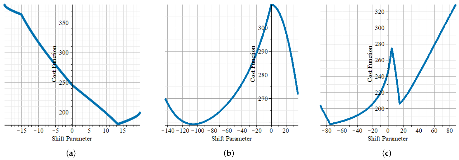
The gimbal lock singularity (6) persists for all values of $\alpha$, but (8) demands $\alpha =0$ or $\alpha =\pi$ so the free parameter is now $\psi \in [-\pi ,\pi ]$ and minimize ${\mathcal{E}}_{\gamma }\left(\psi \right)$ instead. Figure 1a illustrates (32) for a rotation by an angle $\varphi =-{120}^{\circ }$ about the vector $\mathbf{n}\sim {(3,4,5)}^t$. Its minimum ${\mathcal{E}}_{\gamma }\left({\alpha }_0\right)\approx {179.81}^{\circ }$ is reached at ${\alpha }_0\approx {13.49}^{\circ }$, which is about $36.49\%$ more efficient compared to the standard Bryan setting ${\mathcal{E}}_{\gamma }\left(0\right)\approx {245.31}^{\circ }$, and thus the optimal angles are as follows:

$$\phi \approx -{0.16}^{\circ },\vartheta \approx -{75.14}^{\circ },\alpha \approx {13.49}^{\circ },\psi \approx -{91.02}^{\circ }.$$

Next, we consider (17) with ${\mathbf{a}}_1={\mathbf{a}}_3$ oriented along the z-coordinate axis and ${\mathbf{a}}_2$ aligned with $OX$, which yields ${\mathbf{a}}_3^{\prime }=cos\alpha {\widehat{\mathbf{e}}}_z-sin\alpha {\widehat{\mathbf{e}}}_y$ and, hence, for the scalar parameters

$$\begin{array}{c}\hfill {\tau }_1={\displaystyle \frac{r_{31}-r_{21}tan\alpha }{r_{32}-r_{22}tan\alpha \pm \sqrt{{\Delta }^{\prime }}}}=tan{\displaystyle \frac{\phi }{2}},{\tau }_2={\displaystyle \frac{1-r_{33}+r_{23}tan\alpha }{-tan\alpha \pm \sqrt{{\Delta }^{\prime }}}}=tan{\displaystyle \frac{\vartheta +\alpha }{2}}\hfill \\ \hfill {\tau }_3=-{\displaystyle \frac{r_{13}sec\alpha }{r_{23}+r_{33}tan\alpha \mp \sqrt{{\Delta }^{\prime }}}}=tan{\displaystyle \frac{\psi }{2}}\hfill \end{array}$$

(34)

where ${\Delta }^{\prime }={sec}^2\alpha -{(r_{33}-r_{23}tan\alpha )}^2$ and by abuse of notation, we let $r_{ij}$ denote the matrix entries of $\mathcal{R}$ in the standard basis. The shift parameter is now unrestricted $\alpha \in [-\pi ,\pi ]$, since $r_{33}^2+r_{23}^2\le 1$. Consider, for example, a half-turn about ${\displaystyle \mathbf{n}\sim {\left(5,4,3\right)}^t}$ (Figure 1b) with

$${\displaystyle {\mathcal{E}}_{\gamma }\left(\alpha \right)=\left|\alpha \right| + |2arctan{\tau }_1| + |2arctan{\tau }_2-\alpha | + |2arctan{\tau }_3|.}$$

Here $\alpha =0$ is a point of local maximum for ${\mathcal{E}}_{\gamma }\left(\alpha \right)$ and the global minimum at ${\alpha }_0\approx -{105.37}^{\circ }$ produces a total difference of ${\mathcal{E}}_{\gamma }\left(0\right)-{\mathcal{E}}_{\gamma }\left({\alpha }_0\right)\approx {50.65}^{\circ }$, i.e., approximately $16.35\%$ decrease in energy consumption or approximately $19.54\%$ increase in efficiency compared to the standard Euler decomposition. The two points of discontinuity ${\alpha }_1\approx -{143.13}^{\circ }$ and ${\alpha }_2\approx {36.87}^{\circ }$ are related to the condition $r_{32}^{\prime }=g_{32}^{\prime }$ ($\phi =0$). The optimal sequence has the following form:

$$\phi \approx -{52.24}^{\circ },\vartheta \approx -{50.77}^{\circ },\psi \approx -{50.77}^{\circ },\alpha \approx -{105.37}^{\circ }.$$

Finally, for the $XYZX$ decomposition setting in Formula (25) one has

$$\begin{array}{c}\hfill {\tau }_1={\displaystyle \frac{r_{32}-r_{23}{tan}^2\alpha +(r_{33}-r_{22})tan\alpha }{r_{33}+r_{22}{tan}^2\alpha -(r_{32}+r_{23})tan\alpha \pm sec\alpha \sqrt{{\Delta }^{″}}}}=tan{\displaystyle \frac{\phi +\alpha }{2}}\hfill \\ \hfill {\tau }_2={\displaystyle \frac{r_{21}tan\alpha -r_{31}}{sec\alpha \pm \sqrt{{\Delta }^{″}}}}=tan{\displaystyle \frac{\vartheta }{2}},{\tau }_3={\displaystyle \frac{r_{21}+r_{31}tan\alpha }{r_{11}sec\alpha \pm \sqrt{{\Delta }^{″}}}}=tan{\displaystyle \frac{\psi }{2}}\hfill \end{array}$$

(35)

with ${\Delta }^{″}={sec}^2\alpha -{(r_{31}-r_{21}tan\alpha )}^2$. Since the condition $r_{11}=0$ holds, the endpoints of the interval for $\alpha$ correspond to the gimbal lock singularity. Consider again the former rotation discussed above in this section (Figure 1c). The minimum at ${\alpha }_0\approx -{74.97}^{\circ }$ yields an increase in efficiency of about $35.82\%$, and the optimal sequence of rotation angles is as follows:

$$\phi \approx ={2.39}^{\circ },\vartheta \approx -{0.18}^{\circ },\psi \approx -{103.3}^{\circ },\alpha \approx -{74.8}^{\circ }.$$

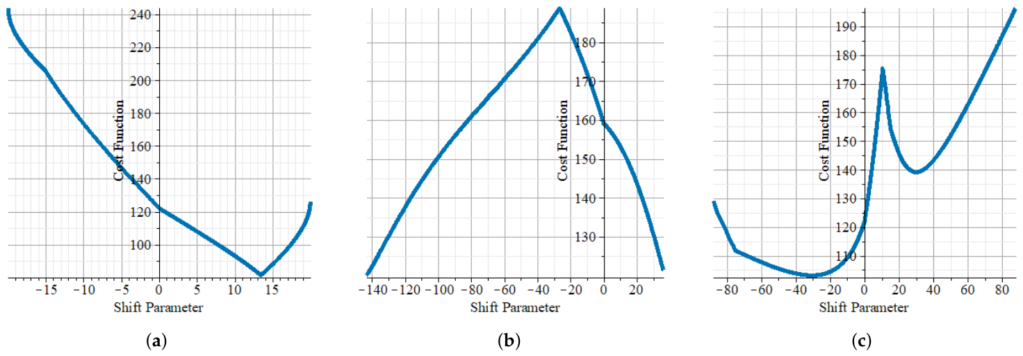
The cost functions (32) in all the examples above imply spherical or cylindrical symmetry, but in the case of significant anisotropy, this is no longer the case due to different moments of inertia or external forces. This can be modeled by introducing different weights:

$${\mathcal{E}}_{\gamma }={\kappa }_1\left(\right|\phi |+\left|\alpha \right|)+{\kappa }_2\left|\vartheta \right|+{\kappa }_3\left|\psi \right|,{\kappa }_i\in [0,1].$$

Figure 2 illustrates this idea. Note that two of the graphs only undergo a slight deformation, while in Figure 2b, we see a phase shift of $\alpha =0$ (from a maximum to an inflection point).

A large part of this section revises an old result by the author, and having the formulas written explicitly here instead of referring to different pages elsewhere should be helpful for a smooth transition to the case of screw motions, considered in the next section. Most of the results follow from the transfer principle, but there are still some subtleties to point out.

4. Dual Quaternions, Screws, and the Transfer Principle

This section is dedicated to implementing the dual extension and applying the transfer principle, which would generalize the above results concerning pure rotations to arbitrary rigid transformations, interpreted as screw motions in view of the famous Mozzi–Chasles theorem. We begin with the construction of dual numbers $\mathbb{R}\left[\epsilon \right]$ as a central extension to $\mathbb{R}$ with a nilpotent element $\epsilon$ (with ${\epsilon }^2=0$) such that for each $\underline{x}=x+y\epsilon \in \mathbb{R}\left[\epsilon \right]$ we refer to $x=Re\left(\underline{x}\right)$ as the real part of $\underline{x}$ and $y=Du\left(\underline{x}\right)$ as its dual part. We may also define the dual conjugate as ${\underline{x}}^{*}=x-y\epsilon$ in analogy with complex numbers, so that $2Re\left(\underline{x}\right)=\underline{x}+{\underline{x}}^{*}$, but retrieving the dual part is less trivial since ${\epsilon }^{-1}$ does not exist. Next, we study the extension to mappings. In particular, for a differentiable function $f\left(x\right)$, we have a finite Taylor series:

$$f(x+y\epsilon )=f\left(x\right)+f^{\prime }\left(x\right)y\epsilon$$

(36)

due to the defining property of $\epsilon$. This yields, for example, the trigonometric identities

$$sin(\phi +\epsilon d)=sin\phi +\epsilon dcos\phi ,cos(\phi +\epsilon d)=cos\phi -\epsilon dsin\phi .$$

(37)

Once we have the construction for real numbers, it is rather straightforward to define $\mathbb{C}\left[\epsilon \right]$, $\mathbb{H}\left[\epsilon \right]$, dual vectors and matrices, etc. In particular, the description of 3D Euclidean motions (rigid displacement) uses unit dual quaternions, which constitute the unit dual 3-sphere:

$${\mathbb{S}}^3\left[\epsilon \right]=\{\underline{\mathcal{Q}}\in \mathbb{H}\left[\epsilon \right],|\underline{\mathcal{Q}}{|}^2={\underline{\mathcal{Q}}}^{†}\underline{\mathcal{Q}}=1\}$$

(38)

and are, in essence, pairs of unit and pure quaternions (see [10] for more details)

$$\underline{\mathcal{Q}}=\left(1+{\displaystyle \frac{\epsilon }{2}}t\right)q,{\left|q\right|}^2=1,t^{†}=-t,{\epsilon }^2=0$$

(39)

where q and t represent rotations and translations, respectively. Consider the dual vector

$$\underline{\mathbf{n}}=\mathbf{n}+\epsilon \mathbf{m}\in {\mathbb{S}}^2\left[\epsilon \right]\iff {\mathbf{n}}^2=1,\mathbf{m}\perp \mathbf{n}$$

(40)

and the dual angle $\underline{\phi }=\phi +\epsilon d$ linked to screw displacement d and moment $\mathbf{m}$ defined as

$$d=\mathbf{t}·\mathbf{n},\mathbf{m}={\displaystyle \frac{1}{2}}\left(cot{\displaystyle \frac{\phi }{2}}-\mathbf{n}\times \right){\mathcal{P}}_{\mathbf{n}}^{\perp }\mathbf{t}$$

(41)

with ${\mathcal{P}}_{\mathbf{n}}^{\perp }$ denoting the orthogonal projector associated with $\mathbf{n}$. Hence, the grade projections

$${\langle \underline{\mathcal{Q}}\rangle }_0=q_0-{\displaystyle \frac{\epsilon }{2}}d=cos{\displaystyle \frac{\underline{\phi }}{2}},{\langle \underline{\mathcal{Q}}\rangle }_2=\mathbf{q}+{\displaystyle \frac{\epsilon }{2}}\left(q_0-\mathbf{q}\times \right)\mathbf{t}=\underline{\mathbf{n}}sin{\displaystyle \frac{\underline{\phi }}{2}}$$

(42)

for which we use the correspondence ${\langle q\rangle }_2\iff \mathbf{q}$, Formula (39), as well as the identities (37). The famous Mozzi–Chasles theorem asserts that each rigid motion can be represented as a screw displacement, i.e., a rotation and translation with a common axis. This so-called ‘screw axis’ is denoted with $\underline{\mathbf{n}}$ above, and the dual quaternion construction provides its Plücker coordinates, while the dual angle $\underline{\phi }$ encodes both the rotational and translational components of this motion. We can derive this information from the dual quaternion and conversely, substitute it in Formula (42), or use some other familiar representation, e.g., $exp\left(\underline{\phi }{\underline{\mathbf{n}}}^{\times }\right)$ for the explicit form of rigid motions. This analogy is guaranteed by the famous Kotelnikov’s principle of transference (or simply ‘transfer principle’), allowing us to extend all known results for classical quaternions to their dual version, as long as the real part is non-vanishing (otherwise one needs to be concerned with zero divisors). Of course, pure translations may also be incorporated, but with a little bit of caution, as we shall see below.

4.1. The Classical Decomposition of Screw Displacements

We begin with generalizing the older result of Euler-type decompositions to the entire Galilean group, using dual quaternions and, more precisely, their projective version. Given three points on the dual sphere ${\underline{\mathbf{a}}}_k\in {\mathbb{S}}^2\left[\epsilon \right]$ interpreted as oriented screw axes, and one in dual projective space $\underline{\mathbf{c}}\in {\mathbb{RP}}^3\left[\epsilon \right]$, we want to find the values of the scalar parameters ${\underline{\tau }}_k\in {\mathbb{RP}}^1\left[\epsilon \right]$ (if they exist), so that the rigid transformation presented by $\underline{\mathbf{c}}$ is factorized as

$$\underline{\mathbf{c}}=\langle {\underline{\mathbf{c}}}_3,{\underline{\mathbf{c}}}_2,{\underline{\mathbf{c}}}_1\rangle ,{\underline{\mathbf{c}}}_k={\underline{\tau }}_k{\underline{\mathbf{a}}}_k$$

(43)

where we use the associativity of the composition law (2), now extended to the non-homogeneous setting via Kotelnikov’s principle of transference. By the same argument, we can also use the Formula (1) to derive the solutions (3). Note that condition (4) remains valid only for the real part of the discriminant $\underline{\Delta }=\Delta +\psi \epsilon$, since from (36), we have

$$\sqrt{\Delta +\psi \epsilon }=\sqrt{\Delta }+{\displaystyle \frac{\psi \epsilon }{2\sqrt{\Delta }}}$$

(44)

where $\psi =Du\left(\underline{\Delta }\right)$ can be easily calculated from the components, that is,

$$\begin{array}{ccc}\hfill {\underline{\mathbf{a}}}_i={\mathbf{a}}_i+\epsilon {\mathbf{b}}_i& \Rightarrow & {\underline{g}}_{ij}={\underline{\mathbf{a}}}_i·{\underline{\mathbf{a}}}_j={\mathbf{a}}_i·{\mathbf{a}}_j+\epsilon ({\mathbf{a}}_i·{\mathbf{b}}_j+{\mathbf{b}}_i·{\mathbf{a}}_j)=g_{ij}+\epsilon h_{ij}\hfill \\ \hfill \underline{\mathcal{R}}=\mathcal{R}+\epsilon \mathcal{S}& \Rightarrow & {\underline{r}}_{ij}={\mathbf{a}}_i·\mathcal{R}{\mathbf{a}}_j+\epsilon \left({\mathbf{a}}_i·\mathcal{R}{\mathbf{b}}_j+{\mathbf{b}}_i·\mathcal{R}{\mathbf{a}}_j+{\mathbf{a}}_i·\mathcal{S}{\mathbf{a}}_j\right)=r_{ij}+\epsilon s_{ij}\hfill \end{array}$$

ultimately leading to

$$\psi =g_{12}{g}_{23}{s}_{31}+(g_{12}{h}_{23}+h_{12}{g}_{23})r_{31}-2(g_{12}{h}_{12}+g_{23}{h}_{23}+r_{31}{s}_{31}).$$

(45)

Similarly, the dual Rodrigues’ vector is given as follows:

$$\underline{\mathbf{c}}=\mathbf{c}+\epsilon \mathbf{d}=tan{\displaystyle \frac{\varphi }{2}}\left(1+{\displaystyle \frac{\epsilon d}{sin\varphi }}\right)\underline{\mathbf{n}},\mathbf{d}={\displaystyle \frac{d\mathbf{n}+sin\varphi \mathbf{m}}{1+cos\varphi }}$$

(46)

which yields ${\underline{\mathbf{c}}}^2={\mathbf{c}}^2(1+2p\epsilon )$, where $p=dcsc\varphi$ denotes the screw pitch, and, respectively

$$\mathcal{S}\left(\underline{\mathbf{c}}\right)=dsin\varphi \left(\mathbf{n}{\mathbf{n}}^t-1\right)+(1-cos\varphi )\left(\mathbf{n}{\mathbf{m}}^t+\mathbf{m}{\mathbf{n}}^t\right)+dcos\varphi {\mathbf{n}}^{\times }+sin\varphi {\mathbf{m}}^{\times }.$$

(47)

Note, however, that the pitch p is ill-defined at both $\varphi =0$ and $\varphi =\pi$, thus it is necessary to clarify the construction for the Rodrigues’ vector itself at these points, unlike in the case of pure rotations, where they represent the trivial element and a half-turn, respectively. At $\varphi =0$ and $d\ne 0$, one has a pure translation, for which the Rodrigues’ vector takes the following form:

$${\underline{\mathbf{c}}}_i={\displaystyle \frac{\epsilon d_i}{2}}{\mathbf{n}}_i\Rightarrow \langle {\underline{\mathbf{c}}}_1,{\underline{\mathbf{c}}}_2\rangle =\langle {\underline{\mathbf{c}}}_2,{\underline{\mathbf{c}}}_1\rangle ={\displaystyle \frac{\epsilon }{2}}\left(d_1{\mathbf{n}}_1+d_2{\mathbf{n}}_2\right)$$

(48)

while in the case of half-turn screws, although (46) is at infinity, (1) is easily expressed as

$$\underline{\mathcal{R}}\left(\underline{\mathbf{c}}\right)=2\underline{\mathbf{n}}{\underline{\mathbf{n}}}^t-\epsilon d{\mathbf{n}}^{\times }-1,\varphi =\pi .$$

(49)

More generally, when extended to the dual setting, the composition law (2) yields

$$\langle {\underline{\mathbf{c}}}_2,{\underline{\mathbf{c}}}_1\rangle =\left(1+\epsilon {\lambda }_{\circ }\right)\langle {\mathbf{c}}_2,{\mathbf{c}}_1\rangle +\epsilon \lambda$$

(50)

with the notation

$${\displaystyle {\lambda }_{\circ }({\underline{\mathbf{c}}}_1,{\underline{\mathbf{c}}}_2)=\frac{{\mathbf{c}}_2·{\mathbf{d}}_1+{\mathbf{d}}_2·{\mathbf{c}}_1}{1-{\mathbf{c}}_2·{\mathbf{c}}_1},\lambda ({\underline{\mathbf{c}}}_1,{\underline{\mathbf{c}}}_2)=\frac{{\mathbf{d}}_2+{\mathbf{d}}_1+{\mathbf{c}}_2\times {\mathbf{d}}_1+{\mathbf{d}}_2\times {\mathbf{c}}_1}{1-{\mathbf{c}}_2·{\mathbf{c}}_1}}$$

and clearly, whenever ${\mathbf{c}}_2·{\mathbf{c}}_1=1$, one ends up with a transformation of the type (49).

If the condition ${\underline{r}}_{21}={\underline{g}}_{21}$ holds, we may use an alternative expression to (5) (see [5]):

$${\underline{\tau }}_1={\displaystyle \frac{{\underline{\mathbf{a}}}_1\times {\underline{\mathbf{a}}}_2·\underline{\mathbf{c}}}{{\underline{g}}_{12}{\underline{\rho }}_1-{\underline{\rho }}_2}},{\underline{\tau }}_2={\displaystyle \frac{{\underline{\mathbf{a}}}_1\times {\underline{\mathbf{a}}}_2·\underline{\mathbf{c}}}{{\underline{g}}_{12}{\underline{\rho }}_2-{\underline{\rho }}_1}}$$

(51)

where ${\underline{\rho }}_i={\underline{\mathbf{a}}}_i·\underline{\mathbf{c}}$, to derive the solution more easily. These are further simplified in the case of orthogonal screw axes ${\underline{g}}_{12}=0$, while $Re({\underline{\rho }}_{1,2})=0$ obviously leads to infinite elements, i.e., transformations of the type (49). Also, in the case ${\omega }_2\ne 0$, one has non-trivial closed rotation sequences (see [4]) which may be extended to closed rigid motion sequences with

$${\underline{\tau }}_1=\underline{\omega }{\underline{\mathsf{\Omega }}}_{23}^{-1},{\underline{\tau }}_2=\underline{\omega }{\underline{\mathsf{\Omega }}}_{31}^{-1},{\underline{\tau }}_3=\underline{\omega }{\underline{\mathsf{\Omega }}}_{12}^{-1}$$

(52)

where ${\underline{\mathsf{\Omega }}}_{ij}$ are the co-factors in the Gram determinant $\underline{\omega }={\underline{\omega }}_2$, e.g., ${\underline{\mathsf{\Omega }}}_{23}={\underline{g}}_{12}{\underline{g}}_{31}-{\underline{g}}_{23}$ etc. This setting may be further generalized by allowing a non-vanishing dual counterpart in the resulting transformation, i.e., factorizing a pure translation into three rigid motions with a non-trivial rotational component. However, neither of these is possible in the degenerate case $\underline{\omega }=0$, although formally we have a solution for ${\underline{\mathbf{a}}}_3=\pm {\underline{\mathbf{a}}}_1$ with ${\underline{\tau }}_3=\mp {\underline{\tau }}_1$ and ${\underline{\tau }}_2=0$.

The gimbal lock singularity also persists in the dual setting, given by the condition

$${\underline{\mathbf{a}}}_3=\pm \underline{\mathcal{R}}{\underline{\mathbf{a}}}_1$$

(53)

in which case the first expression in (51) yields the dual scalar parameter for ${\underline{\varphi }}_1\pm {\underline{\varphi }}_3$, respectively. We now consider a couple of examples before discussing the case of four factors.

Let us begin we a pair of screw axes given by ${\underline{\mathbf{a}}}_1={(0,1,-\epsilon )}^t$${\underline{\mathbf{a}}}_2={(1,0,\epsilon )}^t$, and a screw motion introduced with its dual Rodrigues’ vector representing a rotation (the displacement is zero since $Du\left({\underline{\mathbf{c}}}^2\right)=0$.) by an angle $\varphi ={\displaystyle \frac{\pi }{3}}$ about a screw axis given by its direction vector $Re\left(\underline{\mathbf{c}}\right)$ and moment $Du\left(\underline{\mathbf{c}}\right)$. We calculate the matrix entries and find that the condition ${\underline{r}}_{21}={\underline{g}}_{21}$ is satisfied, so a decomposition into a pair of screw motions exists with scalar parameters ${\tau }_{1,2}=1\pm \epsilon$ easily obtained using Formula (51). Hence, one has $\underline{\mathbf{c}}=\langle {\underline{\mathbf{c}}}_2,{\underline{\mathbf{c}}}_1\rangle$ with ${\underline{\mathbf{c}}}_1={(0,1+\epsilon ,-\epsilon )}^t$ and ${\underline{\mathbf{c}}}_2={(1-\epsilon ,0,\epsilon )}^t$ as can be easily verified by (2), or in matrix terms, using (1) we can write

$$\mathcal{R}\left(\underline{\mathbf{c}}\right)=\left(\begin{array}{ccc}\hfill -2\epsilon & \hfill 0& \hfill 1\\ \hfill 1& \hfill 2\epsilon & \hfill 2\epsilon \\ \hfill -2\epsilon & \hfill 1& \hfill 0\end{array}\right)=\left(\begin{array}{ccc}\hfill 1& \hfill -\epsilon & \hfill \epsilon \\ \hfill \epsilon & \hfill \epsilon & \hfill -1\\ \hfill \epsilon & \hfill 1& \hfill \epsilon \end{array}\right)\left(\begin{array}{ccc}\hfill -\epsilon & \hfill \epsilon & \hfill 1\\ \hfill -\epsilon & \hfill 1& \hfill -\epsilon \\ \hfill -1& \hfill -\epsilon & \hfill -\epsilon \end{array}\right)=\mathcal{R}\left({\underline{\mathbf{c}}}_2\right)\mathcal{R}\left({\underline{\mathbf{c}}}_1\right).$$

Geometrically, ${\underline{\mathbf{c}}}_1$ and ${\underline{\mathbf{c}}}_2$ are interpreted as screw motions with quarter-turn rotational components and displacements $d_{1,2}=\pm 1$, as can be seen from (46). Next, we consider a decomposition into three factors $\mathcal{R}\left(\underline{\mathbf{c}}\right)=\mathcal{R}\left({\underline{\mathbf{c}}}_3\right)\mathcal{R}\left({\underline{\mathbf{c}}}_2\right)\mathcal{R}\left({\underline{\mathbf{c}}}_1\right)$ where ${\underline{\mathbf{a}}}_3={\underline{\mathbf{a}}}_1$ and $\mathcal{R}$ is a rigid transformation of type (49) with a screw line $\underline{\mathbf{n}}={\displaystyle \frac{1}{\sqrt{2}}}{(1+\epsilon ,1-\epsilon ,0)}^t$. Here, the Davenport condition ${\underline{g}}_{12}={\underline{g}}_{13}=0$ is satisfied with $\underline{\Delta }=1$ and since ${\underline{\omega }}_i\equiv 0$ the solutions (3) are symmetric: ${\underline{\tau }}_1^{\pm }={\underline{\tau }}_3^{\pm }=\pm 1$ and ${\tau }_2^{\pm }=\pm (1+2\epsilon )$, which yields the matrix factorization

$$\left(\begin{array}{ccc}\hfill 2\epsilon & \hfill 1& \hfill 0\\ \hfill 1& \hfill -2\epsilon & \hfill 0\\ \hfill 0& \hfill 0& \hfill -1\end{array}\right)=\left(\begin{array}{ccc}\hfill 0& \hfill \epsilon & \hfill 1\\ \hfill -\epsilon & \hfill 1& \hfill -\epsilon \\ \hfill -1& \hfill -\epsilon & \hfill 0\end{array}\right)\left(\begin{array}{ccc}\hfill 1& \hfill -\epsilon & \hfill \epsilon \\ \hfill \epsilon & \hfill -2\epsilon & \hfill -1\\ \hfill \epsilon & \hfill 1& \hfill -2\epsilon \end{array}\right)\left(\begin{array}{ccc}\hfill 0& \hfill \epsilon & \hfill 1\\ \hfill -\epsilon & \hfill 1& \hfill -\epsilon \\ \hfill -1& \hfill -\epsilon & \hfill 0\end{array}\right)$$

along with its transpose (note that the matrix on the left is symmetric since $d=0$). Geometrically, the outer factor represents a quarter-turn about a screw axis given by its Plücker coordinates $Re\left({\underline{\mathbf{a}}}_1\right)$ and $Du\left({\underline{\mathbf{a}}}_1\right)$, while the one in the middle has a non-trivial displacement $d_2^{\pm }=\pm 2$ beside the quarter-turn rotation ${\varphi }_2^{\pm }=\pm {\displaystyle \frac{\pi }{2}}$, and its moment vector is $\mathbf{m}={(0,0,1)}^t$.

The transfer principle certainly allows us to do much more with dual matrices and quaternions. For interesting examples and possible applications, we refer the reader to [8,9,10] and focus on generalizing what we previously called ‘the shift parameter’ construction.

4.2. Optimization of Screw Motions

We begin with the observation that Formula (4), which provides the necessary and sufficient condition for factorization in $\mathrm{SO}\left(3\right)$, remains valid also in the case of generic rigid (screw) motions, since only the real part of the determinant actually remains under the square root, as Formula (44) shows. Hence, all inequalities regarding the relative angles, such as (12) or (28), also apply in this broader setting. It may seem counterintuitive since pure translations cannot always be factorized unless the axes form a system of maximal rank, but that case goes beyond the validity of the transfer principle we rely on here, and yet, it is still possible in some cases, accounting for mutually canceling rotational components in the decomposition. This can be considered as a variation of a closed rotation sequence solution which exists in two cases: non-coplanar axes, where Formula (52) applies, and ${\underline{\mathbf{a}}}_3=\pm {\underline{\mathbf{a}}}_1$ with direct cancellation ${\tau }_3=\mp {\tau }_1$, ${\tau }_2=0$, leaving room for a residual slide, e.g.,

$$\langle {\mathbf{e}}_1+\epsilon {\mathbf{e}}_2,-{\mathbf{e}}_1+\epsilon {\mathbf{e}}_2\rangle =\epsilon \left({\mathbf{e}}_2+{\mathbf{e}}_3\right).$$

Having pointed this out, let us return to the regular case of screw motions with non-vanishing rotational component $\varphi \ne 0$. All equalities derived in the previous section generalize for the corresponding dual entities ${\underline{g}}_{ij}$, ${\underline{r}}_{ij}$, etc., while the inequalities apply for their real counterparts. Consider, for example, the decomposition (33) for a screw motion determined by its dual Rodrigues’ vector $\underline{\mathbf{c}}={(1,1+\epsilon ,1-\epsilon )}^t$, which is obviously a rotation by an angle $\varphi ={\displaystyle \frac{\pi }{3}}$ about a screw axis with Plücker coordinates $Re\left(\underline{\mathbf{c}}\right)$ and $Du\left(\underline{\mathbf{c}}\right)$. Let ${\tau }_i\left(\alpha \right)={\tau }_i^{+}$, so that ${\tau }_1\left(0\right)=1+\epsilon$, ${\tau }_2\left(0\right)={\displaystyle \frac{\epsilon }{2}}$ and ${\tau }_3\left(0\right)=1$, i.e., the decomposition involves a quarter-turn, a translation, and a screw motion with ${\sum }_{i=1}^3\left|{\varphi }_i\right|=\pi$, ${\sum }_{i=1}^3\left|d_i\right|={\displaystyle \frac{3}{2}}$, namely

$$\left(\begin{array}{ccc}\hfill 0& \hfill \epsilon & \hfill 1\\ \hfill 1& \hfill \epsilon & \hfill 0\\ \hfill -\epsilon & \hfill 1& \hfill -\epsilon \end{array}\right)=\left(\begin{array}{ccc}\hfill 0& \hfill -1& \hfill 0\\ \hfill 1& \hfill 0& \hfill 0\\ \hfill 0& \hfill 0& \hfill 1\end{array}\right)\left(\begin{array}{ccc}\hfill 1& \hfill 0& \hfill \epsilon \\ \hfill 0& \hfill 1& \hfill 0\\ \hfill -\epsilon & \hfill 0& \hfill 1\end{array}\right)\left(\begin{array}{ccc}\hfill 1& \hfill 0& \hfill 0\\ \hfill 0& \hfill -\epsilon & \hfill -1\\ \hfill 0& \hfill 1& \hfill -\epsilon \end{array}\right)·$$

It is interesting to observe that in this case ${\tau }_1=1+\epsilon$ does not depend on $\alpha$, while ${\tau }_2={\displaystyle \frac{\epsilon }{2cos\alpha }}$ and ${\tau }_3=1-\epsilon tan\alpha$, so the minimum (with respect to both degrees of freedom) is at $\alpha =0$. Interestingly enough, if we use the basis $\left\{{\underline{\mathbf{a}}}_i\right\}$ from our previous example, there is a stable factorization into a pair of screw motions $\underline{\mathbf{c}}=\langle (\epsilon -1){\underline{\mathbf{a}}}_3,(1+\epsilon ){\underline{\mathbf{a}}}_2\rangle$ that are not affected by $\alpha$.

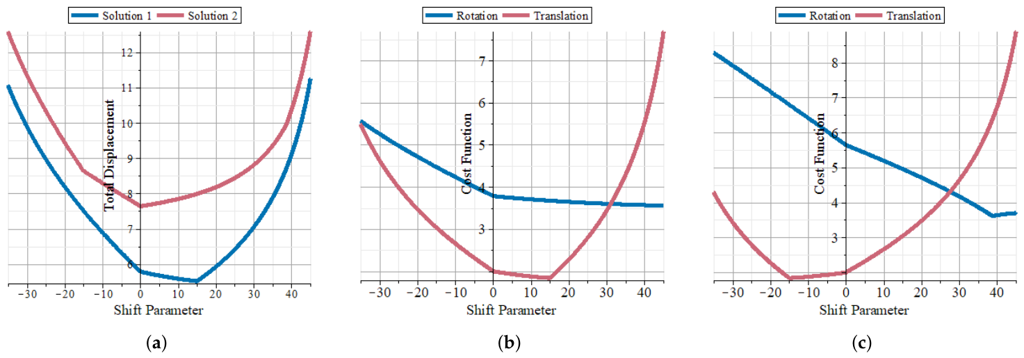
Our next example illustrates how both the total rotation and total displacement in a screw decomposition can be independently affected by the additional parameter $\alpha$, which is kept real (angular) for the sake of representability. For our compound rigid motion, we choose $\underline{\mathbf{c}}={\displaystyle \frac{1}{5}}{(3+4\epsilon ,4-3\epsilon ,\epsilon )}^t$, which is again a quarter-turn about a screw axis with direction vector $Re\left(\underline{\mathbf{c}}\right)$ and moment $Du\left(\underline{\mathbf{c}}\right)$. The decomposition takes place with respect to an orthonormal basis formed by ${\underline{\mathbf{a}}}_1$, ${\underline{\mathbf{a}}}_2$ and ${\underline{\mathbf{a}}}_3={\underline{\mathbf{a}}}_1\times {\underline{\mathbf{a}}}_2$ used in the previous example, so the dual extension of Formula (33) applies here, and it is straightforward to assess the cost functions for the rotation and displacement components in the factorization separately (Figure 3). We should take into account that the minimum with respect to these two counterparts typically does not occur at the same value of $\alpha$, as can be seen in that example, so we have to prioritize according to the actual energy cost associated with these types of motion. This can also be done with the help of statistical weights adjusted to the situation. Another observation worth mentioning is that while the intervals for $\alpha$ are preserved in the dual extensions, the cost function builds up even more rapidly approaching its boundaries compared to the case of pure rotations. Moreover, the solutions may still have discontinuities within these intervals, in analogy with the classical gimbal lock setting, as well as infinite values corresponding to generalized half-turns (49). Note also that with the above example we impose an artificial restriction on $\alpha$ demanding that it is real, which may prevent us from arriving at the optimal solution but is convenient for a nice graphic representation. In our numerical experiments, the overall displacement increases quickly when $\alpha$ is far from zero; however, as in the case of pure rotations, its minimum does not have to be at the origin.

To conclude, let us summarize the whole process in a nutshell. Given a compound rotation $\mathcal{R}$ and a set of invariant axes, one constructs all possible Euler-type decompositions into four factors by permuting the axes and assessing the corresponding condition. For a pair of axes, we only have two such configurations, but for a triplet, we end up with a dozen of them. If all of them satisfy the necessary and sufficient condition, we typically expect a pair of solutions with a free parameter for each configuration, which doubles them to 24, and, finally, assigning the parameter to each of the two repeated axes in the pair (using conjugation wherever necessary) yields the number 48. For each such setting, we have an analytic solution in terms of the ‘shift parameter’ $\alpha$, for which the corresponding cost function can be minimized, and comparing those minima, we pick the best configuration and $\alpha$-value to perform our motion sequence. Needless to say, the cost function itself needs to be determined first: on the one hand, the energy cost of rotation and translation differs, while on the other, so do rotations about different axes in asymmetric rigid bodies. Both of these aspects can be modeled using effective weights, as discussed above. Although this approach may seem confusing, it has some clear advantages, e.g., all solutions are analytic, and optimization may, in principle, be performed symbolically; no iterative procedure is needed—only simple matrix calculations. Moreover, many entries in the parallel solutions, such as $g_{ij}$ and $r_{ij}$, are shared, so there is no need to repeat the same calculations. A block diagram of the proposed method is given for convenience in Figure 4.

Although the idea is quite clear, there are some technicalities to consider in the process. Firstly, for certain values of $\alpha$ within the allowed interval, one may hit a gimbal lock singularity, which is reflected as a discontinuity of the cost function, occurring both in the case of pure rotations and for generic rigid motions. As explained above, this simply transfers freedom from the shift parameter to the one encoded in the gimble lock entanglement (see [5]). Those critical $\alpha$-values may solve our optimization problem in rare cases; more precisely, their left or right limits may provide the global minimum. Secondly, there are an infinite number of points in our description, and that is the price we pay for avoiding redundant parameters. Those infinite points correspond to half-turns or their dual extension (49) and also may appear as optimal solutions, however unlikely. Since we deal with mostly rational expressions, this may be detected by the vanishing denominator, at least in the regular setting (no gimbal lock). L’Hôpital’s rule then provides the correct numerical value. Another way to avoid infinite points is going back to homogeneous (dual quaternion) coordinates or, to be safe, performing a double-valued lift back to the spin cover $\underline{\mathbf{c}}\to {\underline{\zeta }}_{\pm }\in {\mathbb{S}}^3\left[\epsilon \right]$ given in this case as

$$\begin{array}{c}\hfill {\underline{\zeta }}_0^{\pm }=\pm {(1+{\underline{\mathbf{c}}}^2)}^{-{\displaystyle \frac{1}{2}}},{\underline{\zeta }}^{\pm }={\left({\underline{\zeta }}_0^{\mp }\right)}^{-1}{\underline{\mathbf{c}}}^{*}\end{array}$$

(54)

where the Hodge dual is being used to transform the quaternion bi-vector part to a vector and vice versa. The additional component increases the number of computations and makes some expressions less intuitive, but since engineers work extensively with matrices and quaternions rather than Rodrigues’ vectors, it is important to point out this correspondence, too. Moreover, some applications involve directly $\mathrm{SU}\left(2\right)$ factorizations, as discussed below.

5. Discussion

The present study does not consider the general problem of geometric control, but rather, contributes to one very specific aspect of it: namely, optimization of discrete screw motion sequences, generalizing the classic Euler-type rotation sequences in attitude control. Unlike other attempts in this area, it relies on closed-form analytic solutions, so there is no assessment of algorithmic complexity provided in this paper (only simple matrix operations are involved). Its only actual limitation is presented by the interval for the variational parameter $\alpha$, while the presence of gimbal lock singularities or infinite solutions within this interval presents merely a technical issue. Note also that we do not consider other optimization criteria, such as finding the smoothest or fastest trajectory interpolating a rigid motion, for example, although these problems may also be approached using dual quaternions. Instead, we focus only on energy efficiency with just one additional parameter. This approach does not guarantee to provide the global minimum in all possible settings, but it is purely analytic, quite easy to implement, and still rather efficient: our calculations show that it may reduce the cost of a maneuver by 30–40% without the need to invoke complex numerical or machine learning algorithms used in other optimization methods (see [13,21,24]). Moreover, our solutions work with a relaxed version of the classical Davenport factorization condition for orthogonal axes, thus allowing for a wider variety of gimbal settings (such as tetrahedral), which might be useful for engineering applications.

Since our construction naturally extends to the spin covering group $\mathrm{SU}\left(2\right)$, it may be applied to qubits in quantum computing, computer vision, and virtual reality [15,25]. A similar approach can be used for the proper Lorentz group in the plane ${\mathrm{SO}}^{+}(2,1)$ and its spin covering $\mathrm{SL}(2,\mathbb{R})\cong \mathrm{SU}(1,1)$ using the decomposition results obtained in [4]. In that setting, however, one needs to take into account, apart from the gimbal lock, also the isotropic singularity associated with the light cone in ${\mathbb{R}}^{2,1}$, which (unlike the former) is not affected by $\alpha$, being an invariant subspace independent of the ${\tau }_i$’s. The ‘dualization’ procedure works similarly in the hyperbolic setting, extending pseudo-rotations to general Poincaré motions in Minkowski $2+1$ space, but even within the homogeneous component, one has different types of transformations: pure rotations, Lorentz boosts, and isotropic displacements, which makes it harder to construct a meaningful cost function only from first principles, as factorizations in general may involve all three, e.g., the famous Iwasawa decomposition. It is an interesting direction in which this study can be generalized, although the $2+1$ Lorentz group has fewer applications compared to $\mathrm{SO}\left(3\right)$ or ${\mathrm{SO}}^{+}(3,1)$: apart from being used as a toy model for relativity, it plays a role in quantum mechanical scattering, the description of graphenes, and certainly classical hyperbolic geometry. The entire Lorentz group, however, is a bit too wild to tame this way: although the factorizations may be described similarly using complex projective biquaternions, dualization does not have the same meaning; furthermore, the Plücker embedding is not trivial, which means we no longer deal with just plane transformations. However, interpreting the generalized ‘axes’ $\left\{{\mathbf{a}}_k\right\}$ as generators of Abelian subgroups, the factorization problem still makes perfect sense in ${\mathrm{SO}}^{+}(3,1)\cong \mathrm{SO}(3,\mathbb{C})$ as well, and as long as one declares a meaningful cost optimization goal, a similar approach can also be applied to the (homogeneous) relativistic setting—from purely algebraic perspective, it is not so different to the one considered here (see [26,27]). However, all these interesting applications and generalizations, as well as the continuous version of the problem, go beyond the scope of the present study and are left for the future.

6. Conclusions

This paper proposes an exact closed-form solution to the optimization problem of finite rigid motion sequences, which arise in the attitude control of robots, drones, and spacecraft. Spatial rotations and translations are interpreted as screw motions and modeled using projective dual quaternions, also known as dual Rodrigues’ vectors. The goal is to minimize the energy output, measured by the total amount of motion in a sequence of four factors, so we have only one free (dual) parameter. The Euclidean and angular displacements contribute to the cost function with weight coefficients, since the difference in energy output between the two types of motion depends on the specific construction of the mechanism and the environment in which it operates. The same applies to rotations about individual gimbals, which may be associated with different moments of inertia or external sources of asymmetry, leading again to the introduction of weights in the cost function. Our solutions are illustrated with numerical examples, both in the pure rotation and screw motion settings. Specific configurations, such as closed sequences (factorizations of the identity map) or gimbal lock singularities, and the role of infinite points are also discussed.

References

1. Sachkov, Y. Introduction to Geometric Control; Springer Nature: Cham, Switzerland, 2022. [Google Scholar]
2. Piovan, G.; Bullo, F. On Coordinate-Free Rotation Decomposition: Euler Angles about Arbitrary Axes. IEEE Trans. Robot. 2012, 28, 728–733. [Google Scholar]
3. Rezaei, A.; Talaeizadeh, A.; Alasty, A. Comparing the Performance of Quaternion, Rotation Matrix, and Euler Angles Based Attitude PID Controllers for Quadrotors. In Proceedings of the 2024 12th RSI International Conference on Robotics and Mechatronics (ICRoM), Tehran, Iran, 17–19 December 2024; pp. 492–497. [Google Scholar]
4. Brezov, D.; Mladenova, C.; Mladenov, I. A Decoupled Solution to the Generalized Euler Decomposition Problem in R 3 and R 2 , 1 . J. Geom. Symmetry Phys. 2014, 33, 47–78. [Google Scholar]
5. Brezov, D.; Mladenova, C.; Mladenov, I. New Perspective on the Gimbal Lock Problem. AIP Conf. Proc. 2013, 1570, 367–374. [Google Scholar] [CrossRef]
6. Piña, E. Rotations with Rodrigues’ vector. Eur. J. Phys. 2011, 32, 1171–1178. [Google Scholar] [CrossRef]
7. Fathian, K.; Jin, J.; Wee, S.G.; Lee, D.H.; Kim, Y.G.; Gans, N.R. Camera relative pose estimation for visual servoing using quaternions. Robot. Auton. Syst. 2018, 107, 45–62. [Google Scholar] [CrossRef]
8. Wittenburg, J. Kinematics: Theory and Applications; Springer: Berlin/Heidelberg, Germany, 2016. [Google Scholar]
9. Condurache, D.; Cojocari, M.; Ciureanu, I.-A. A Closed Form of Higher-Order Cayley Transforms and Generalized Rodrigues Vectors Parameterization of Rigid Motion. Mathematics 2025, 13, 114. [Google Scholar] [CrossRef]
10. Farias, J.G.; De Pieri, E.; Martins, D. A Review on the Applications of Dual Quaternions. Machines 2024, 12, 402. [Google Scholar] [CrossRef]
11. Valverde, A.; Tsiotras, P. Spacecraft Robot Kinematics Using Dual Quaternions. Robotics 2018, 7, 64. [Google Scholar] [CrossRef]
12. Arrizabalaga, J.; Ryll, M. Pose-Following with Dual Quaternions. In Proceedings of the 2023 62nd IEEE Conference on Decision and Control (CDC), Singapore, 13–15 December 2023; IEEE: Piscataway, NJ, USA, 2023; pp. 5959–5966. [Google Scholar]
13. Condurache, D.; Cojocari, M. The Extended Wahba’s Problem in Dual and Multi-Dual Algebras. In Proceedings of the 2024 10th International Conference on Control, Decision and Information Technologies (CoDIT), Vallette, Malta, 1–4 July 2024; pp. 2108–2113. [Google Scholar]
14. Yang, Y. Spacecraft Modeling, Attitude Determination, and Control: Quaternion-Based Approach, 2nd ed.; CRC Press: Boca Raton, FL, USA, 2025. [Google Scholar]
15. Billig, Y. Time-Optimal Decompositions in SU(2). Quantum Inf. Process. 2013, 12, 955–971. [Google Scholar] [CrossRef]
16. Billig, Y. Optimal Attitude Control with Two Rotation Axes. SIAM J. Control Optim. 2019, 57, 1111–1131. [Google Scholar] [CrossRef]
17. Eslamiat, H.; Wang, N.; Hamrah, R.; Sanyal, A.K. Geometric Integral Attitude Control on SO(3). Electronics 2022, 11, 2821. [Google Scholar] [CrossRef]
18. Zhang, S.; Shi, X.; Chen, X.; He, X. Trajectory Tracking Control Based on Generalized Rodrigues Parameter for Underactuated VTOL UAVs. J. Aerosp. Eng. 2024, 32, 6. [Google Scholar] [CrossRef]
19. Zheng, Z.; Shang, W.; Ai, J.; Zou, Y.; Liu, Z. Integrated Geometric Optimal Control of Spacecraft Attitude and Orbit Based on SE(3). IEEE Access 2023, 11, 27382–27394. [Google Scholar] [CrossRef]
20. Brezov, D. The Order of Finite Generation of SO(3) and Optimization of Rotation Sequences. Rocky Mt. J. Math. 2026, 56, 23–32. [Google Scholar] [CrossRef]
21. Jin, K.; Huang, G.; Lei, R.; Wei, C.; Wang, Y. Multi-constrained predictive optimal control for spacecraft attitude stabilization and tracking with performance guarantees. Aerosp. Sci. Technol. 2024, 155, 109599. [Google Scholar] [CrossRef]
22. Guerrero-Sánchez, M.E.; Abaunza, H.; Castillo, P.; Lozano, R.; García-Beltrán, C.D. Quadrotor Energy-Based Control Laws: A Unit-Quaternion Approach. J. Intell. Robot. Syst. 2017, 88, 347–377. [Google Scholar] [CrossRef]
23. Brezov, D. Optimization and Gimbal Lock Control via Shifted Decomposition of Rotations. J. Appl. Comput. Math. 2018, 7, 410. [Google Scholar]
24. Cai, Y.; Low, K.S.; Wang, Z. Reinforcement Learning-Based Satellite Formation Attitude Control Under Multi-Constraint. Adv. Space Res. 2024, 74, 5819–5836. [Google Scholar] [CrossRef]
25. D’Alessandro, D. Introduction to Quantum Control and Dynamics, 2nd ed.; CRC Press: Boca Raton, FL, USA, 2021. [Google Scholar]
26. Brezov, D. Higher-Dimensional Representations of SL(2, R ) and Its Real Forms via Plücker Embedding. Adv. Appl. Clifford Algebras 2017, 27, 2375–2392. [Google Scholar] [CrossRef]
27. Shariati, A. A Mathematical Approach to Special Relativity; Academic Press: London, UK, 2023. [Google Scholar]
Figure 1. Plot of E γ ( α ) for (a) X Y X Z sequence (7) with ϕ = 120 and n = ( 3 , 4 , 5 ) t , (b) Z X Z X sequence (17) of a half-turn about n = ( 5 , 4 , 3 ) t , and (c) the former rotation in a X Y Z X setting (25).
Appliedmath 06 00080 g001
Figure 2. The examples illustrated in Figure 1 (following the same order) with a modified (weighted) cost function E γ ( α ) . The weight values for the three axes are set to: κ 1 = 1 , κ 2 = 1 / 2 and κ 3 = 1 / 3 .
Appliedmath 06 00080 g002
Figure 3. (a) The weighted cost function for the factorization (7) of c ̲ = 1 5 ( 3 + 4 ε , 4 3 ε , ε ) t in the basis { a ̲ i } , (b,c) depict the rotation and displacement components separately for the two solutions in (33). Angles are measured in radians on the y-axis, and the weights for both types of motion are equal.
Appliedmath 06 00080 g003
Figure 4. A block diagram of the proposed optimization method in five simple steps.
Appliedmath 06 00080 g004
Disclaimer/Publisher’s Note: The statements, opinions and data contained in all publications are solely those of the individual author(s) and contributor(s) and not of MDPI and/or the editor(s). MDPI and/or the editor(s) disclaim responsibility for any injury to people or property resulting from any ideas, methods, instructions or products referred to in the content.