End-to-End Tool Path Generation for Triangular Mesh Surfaces in Five-Axis CNC Machining

Abstract

Triangular mesh surface representation is widely adopted in geometric design and reverse engineering applications. However, in high-precision Computer Numerical Control (CNC) machining, significant limitations persist in automated Computer-Aided Manufacturing (CAM) tool path generation for such representations. Conventional CAM workflows heavily rely on manual engineering interventions, such as creating drive surfaces or tuning extensive parameters—a dependency that becomes particularly acute for generic free-form models. To address this critical challenge, this paper proposes a novel end-to-end single-step end-milling tool path generation methodology for triangular mesh surfaces in high-precision five-axis CNC machining. The framework includes clustering analysis for optimal workpiece orientation, normal vector distribution analysis to identify shallow and steep regions, Graphics Processing Unit (GPU)-accelerated collision detection for feasible tool orientation domains, and iso-planar tool path generation with Traveling Salesman Problem (TSP) optimization for efficient tool lifting and movement. Experimental validation confirms the framework ensures machining quality and algorithmic robustness.

1. Introduction

Subtractive manufacturing for free-form surfaces is a core technology in digital manufacturing and a key bottleneck restricting the development of high-end manufacturing. The numerous mathematical problems involved, such as optimization algorithms, path planning, and geometric modeling, not only have significant theoretical research value but also serve as important technical supports for practical industrial applications. Therefore, theoretical analysis and efficient algorithm design for these mathematical problems hold important academic and practical significance.

The related manufacturing process mainly includes Computer-Aided Design (CAD), Computer-Aided Manufacturing (CAM), post-processing, and triangular meshing-based machining. The machining path in CAM refers to the relative motion trajectory between the workpiece and the machine tool, determining how the tool cuts the blank to form the surface shape specified by the design geometry [1,2]. From the perspective of kinematics, the curvature characteristics of the machining path directly affect the smoothness of the feedrate, while the differential geometric properties of the path envelope surface are strongly coupled with key physical quantities such as instantaneous chip area and cutting force fluctuations. Under the current demand for improving machining accuracy and efficiency, the deep integration of CAD and CAM systems has become an urgent technical requirement in the field of advanced manufacturing. The machining tool path, as a key information carrier linking CAD geometric modeling and CAM process planning, directly affects the precision control and efficiency optimization of the machining process.

With the breakthrough development of 3D scanning and machine vision technologies, reverse engineering and rapid prototyping have become popular technologies in modern intelligent manufacturing systems. This methodology, by constructing high-precision digital twin models of physical entities, significantly shortens the product iteration cycle and reduces trial-and-error costs. The triangular mesh surface, with its simple discrete topological structure and efficient construction characteristics, has evolved into a mature representation for complex geometric modeling in CAD systems.

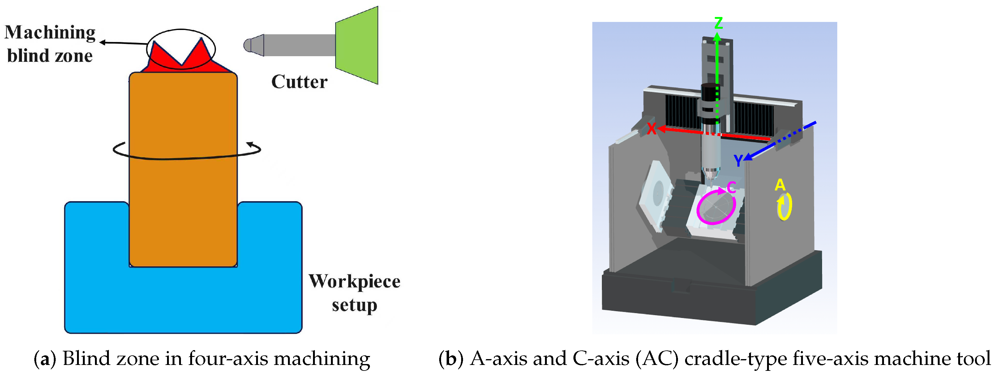
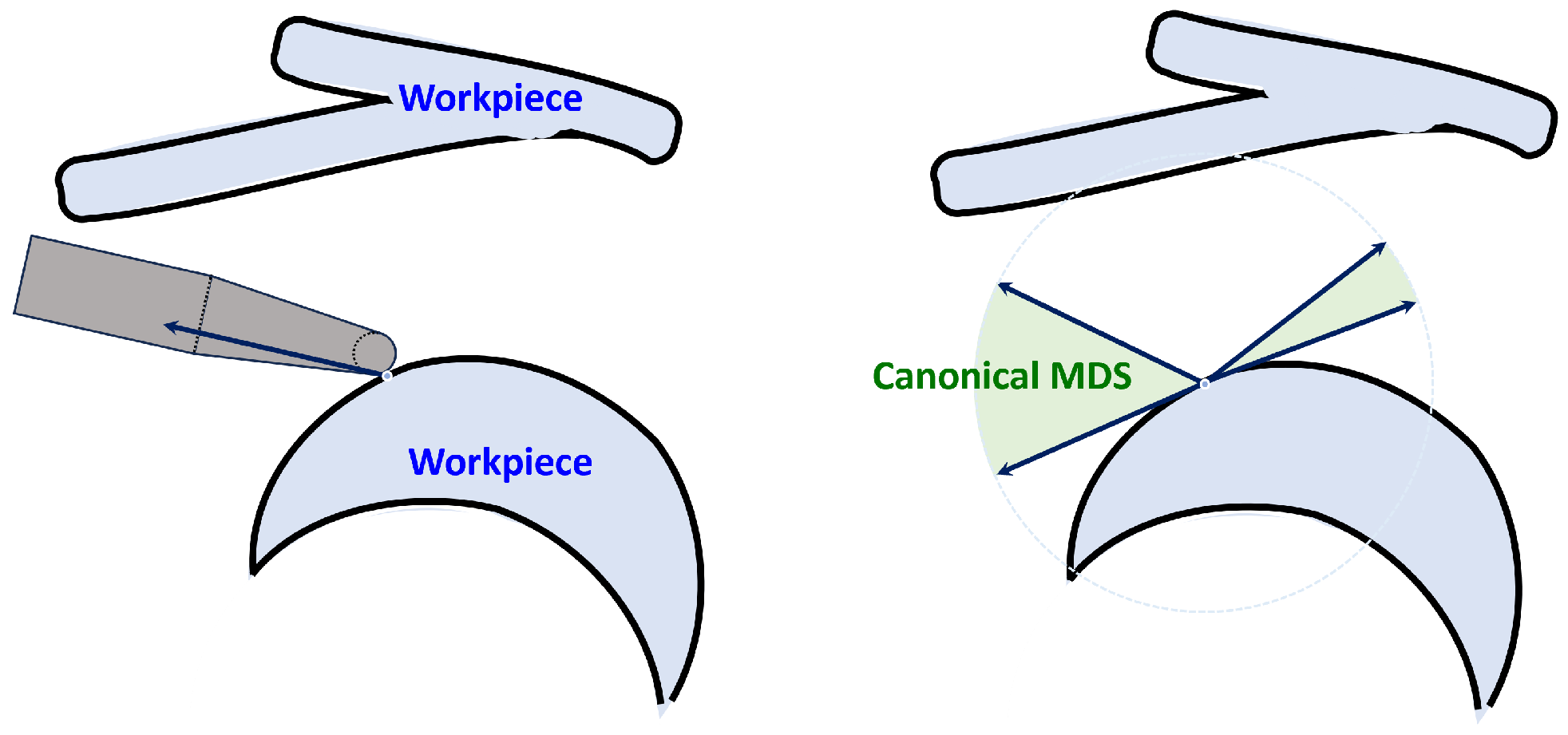
In recent years, tool path planning for CAM machining of triangular mesh surfaces has attracted extensive attention from scholars. For solid models, the traditional machining process includes surface segmentation based on obstacle avoidance and single surface fixed-direction path planning [3,4]. This method effectively decouples the issues of tool axis collision detection and tool path generation, thus ensuring the robustness of the algorithm when handling complex models. However, in this method, due to the use of fixed tool orientations on each surface segment, noticeable scallop material is left at the junctions of surface segments, significantly reducing machining quality [5,6]. To address this issue, four-axis wrapping machining has been proposed in both academia [6] and industry [7], which can effectively improve surface quality. However, these methods, similar to turning machining, create blind spots in shallow areas of the models (where the surface normal is nearly parallel to the main clamping direction), as shown in the Figure 1a. To ensure that the scallop height constraint is met in these areas, such methods often require the accumulation of multiple redundant tool paths, which results in a trade-off between machining efficiency and precision. Furthermore, due to machine tool structural limitations, there are some areas of the model that cannot be machined.

To address this issue, we extend the wrapping machining method to the A-axis and C-axis(AC) cradle-type five-axis machine tool (Figure 1b) and propose an end-to-end integrated end-milling finishing tool path generation method, thereby effectively eliminating machining blind areas. The specific process is as follows: First, we use normal vector clustering analysis to determine the setup direction and divide the machining area into shallow and steep regions based on the distribution characteristics of the sampled point normal vectors; second, we construct an efficient collision detection model based on Graphics Processing Unit (GPU) parallel acceleration, extract the set of feasible machining directions across the surface by discretizing the tool pose space, and obtain the optimal machining direction for the shallow region; finally, we use the iso-plane method to generate tool paths for both shallow and steep regions and construct a tool lifting path generation model with the minimum empty travel time based on the feasible direction domain of the path points, combined with the Traveling Salesman Problem (TSP) global optimization algorithm, under the constraint of the feasible domain of the tool pose, thereby achieving simultaneous optimization of machining efficiency and surface quality. The experimental results verify the effectiveness of this method. In the following paragraphs, Section 2 introduces related work on integrated tool path generation for triangular meshes; Section 3 presents the proposed novel integrated machining path method, which is divided into optimal setup direction, shallow-steep segmentation, tool path generation, and optimal tool lifting/rapid traverse line generation; Section 4 provides the experimental results and comparisons of this method, thereby demonstrating its effectiveness and superiority; Section 5 discusses the superiority of the proposed method and outlines prospective directions for its future improvement.

2. Related Work

Besides the three traditional methods for machining single surface segments (iso-parametric method [8,9], iso-planar method [10,11], iso-scallop height method [12,13,14]), the integrated triangular meshing-based machining can be generally divided into two types: segmentation-based tool path planning and wrapping-based tool path planning. In the former strategy, a key indicator optimizes the number of surface segments to minimize the number of clamping operations. Fanni et al. [15] proposed a surface segmentation method based on polygonal cube mappings (Polycube Mappings) and analyzed the machinability of additive and subtractive manufacturing segmentations, considering both three-axis and four-axis milling. Muntoni et al. [16] redefined the discrete constraint optimization problem of surface segmentation as an unconstrained optimization problem of a continuous function, thereby calculating a set of potentially overlapping height-domain surface segments that jointly cover the model surface. Yang et al. [17] improved machining efficiency by using a more generalized Double Height Field (DHF) slicing method to replace the single-height field segmentation. By minimizing the number of DHF slices and maximizing slice heights, the method can effectively improve machining efficiency.

Moreover, researchers have also considered the selection of machining directions during the surface segmentation process, aiming to minimize the number of surface segments. The problem is transformed into a multi-label graph-cut optimization problem, where an optimal machining direction is assigned to each surface patch based on tool accessibility constraints. This graph-cut based segmentation planning method has proven its effectiveness and robustness in three-axis machining [18], four-axis machining [5], and five-axis machining [3].

For the alternative wrapping machining strategy, related work mainly focuses on four-axis machining and is concentrated in the industrial field (commercial industrial software), with a lack of technical reports due to commercial purposes. Analysis of the results from several commercial software applications shows that Luban [7] handles four-axis machining by utilizing the convex hull of sliced profiles. It generates 360-degree tool paths along the convex hull boundaries for each slice layer and projects them onto the sliced profile. However, experiments show that it can only handle simple geometric models with a single profile per slice and cannot process models with multiple profiles per layer. Autodesk Fusion 360 [19] provides a “rotation” finishing strategy for four-axis machining, allowing users to choose from three types of rotating tool paths: spiral, straight-line, or circular. However, experiments reveal that Fusion 360 cannot generate completely collision-free machining paths, resulting in significant over-cutting and under-cutting. Siemens NX [20] provides a semi-automatic strategy for generating tool paths for CAD models, which requires manual specification of driving geometry or guide curves, and generates tool paths at the feature level. This process involves numerous parameters and requires complex programming. In contrast, in academia, Zhang et al. [6] proposed an end-to-end single-step four-axis tool path generation method, which uniformly slices the model. For each slice, they perform accessibility analysis on each cutting contour within the slice and finally generate the optimal transfer path using a graph-cut or TSP algorithm. However, as mentioned earlier, this method has machining blind spots, and this limitation motivates us to focus on the current research.

3. Methodology

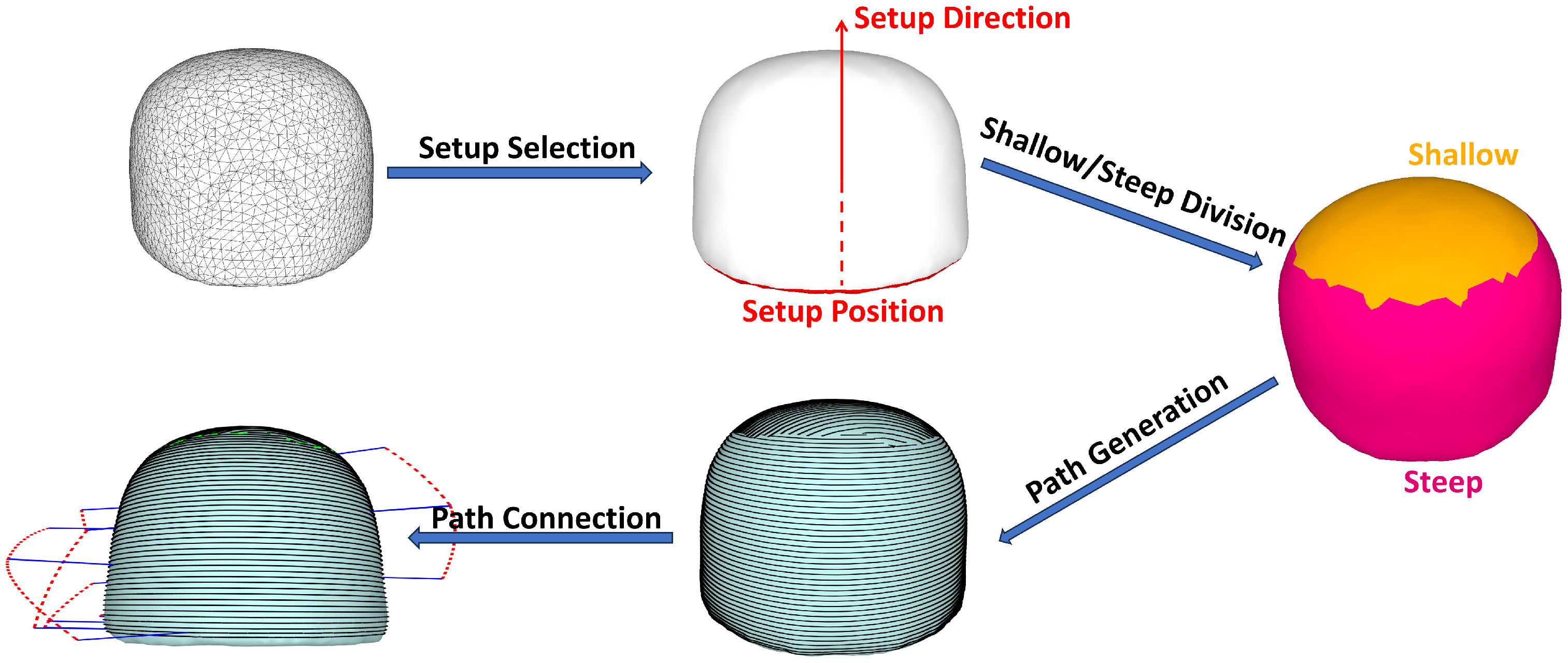
This paper proposes an integrated end-milling tool path generation method for triangular mesh surfaces for a five-axis machine. To clearly illustrate the proposed algorithm, a simple semi-ellipsoid model is introduced as a running example in this section. The complex models like the Bunny (used in previous works) will be reserved for Section 4 to demonstrate the algorithm’s capability on generic free-form surfaces. The method includes four main steps: (1) optimal setup direction selection; (2) shallow and steep boundary division; (3) tool path segment generation; and (4) path segment connection based on TSP. The evolution of the semi-ellipsoid model through these steps is illustrated in Figure 2.

3.1. Optimal Setup Direction Selection

In practical Computer Numerical Control (CNC) machining scenarios, the first step is to select a part of the model as the base for setup, while the remaining part is to be machined. The setup base should be as flat as possible and have a large area. Therefore, we use a two-stage clustering method to determine the optimal setup base and the setup direction perpendicular to it.

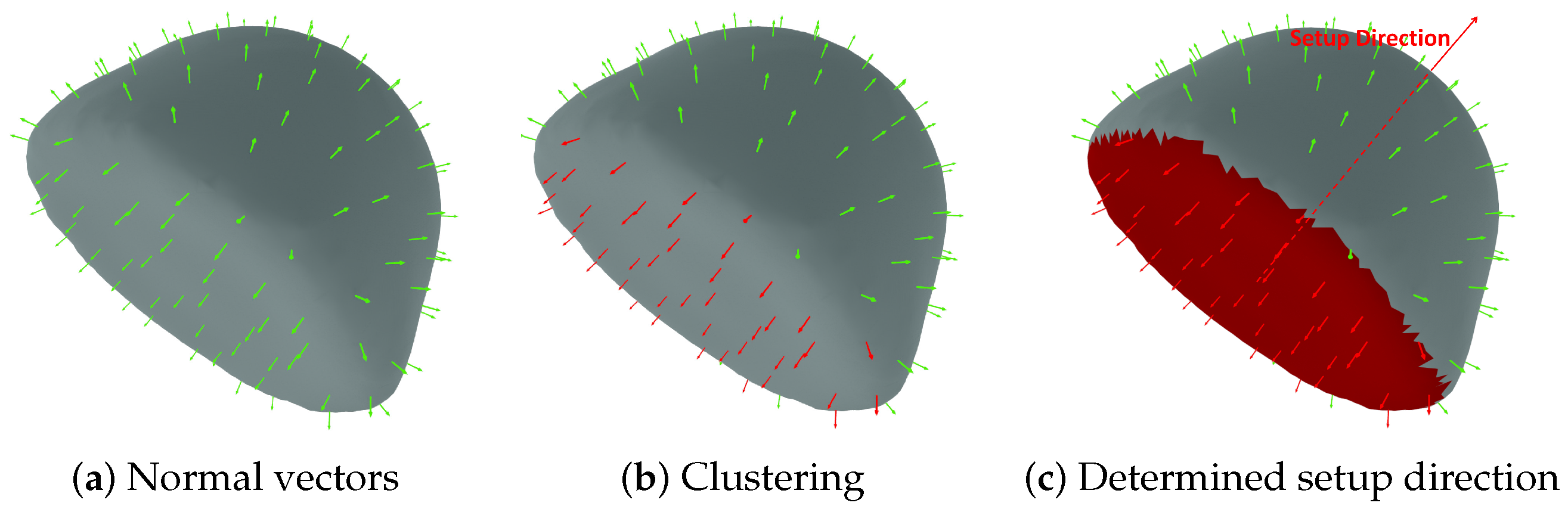
In the first stage, we calculate the normal vectors of each triangular face in the model and treat each normal vector as a data point in three-dimensional Euclidean space. Taking the semi-ellipsoid model as an example, the normal vectors on the flat bottom surface are approximately parallel to the negative Z-axis. We then use the k-means clustering algorithm to classify these data points automatically. Figure 3a visualizes the distribution of these normal vectors on the model, where the clustering algorithm can easily identify the main cluster corresponding to the bottom surfaces.

After clustering, we construct the following feature evaluation function to quantify the clusters:

$$\begin{array}{c}\hfill \epsilon =\mu ·S-\gamma ·\Gamma ,\end{array}$$

(1)

where the term S is average distance from the data points within a cluster to the cluster center, which represents the intra-cluster similarity. $\Gamma$ denotes the number of data points in the cluster. $\mu$ and $\gamma$ are weighting coefficients. The cluster that minimizes the evaluation function is considered the optimal cluster, and the direction of its centroid is used as the setup direction. In the semi-ellipsoid case, the cluster corresponding to the flat bottom surface has a minimal S (high flatness) and a large $\Gamma$ (large area), making it the optimal choice according to the evaluation function. Consequently, the direction perpendicular to this base is selected as the setup direction, as shown in Figure 3c. Following the parameter settings in [21], we set $\mu =0.7$ and $\gamma =0.3$, which have been experimentally verified to effectively balance the trade-off between the consistency of the setup base’s normal vector (representing flatness) and the size of its area.

However, the cluster determined in the first stage may map to multiple disconnected regions on the model surface (such as the top of the semi-ellipsoid model). Therefore, a secondary clustering is performed based on the height of the triangular faces corresponding to the optimal cluster in the setup direction. The cluster with the lowest average height is selected as the final model setup base.

The detailed procedure is outlined in Algorithm 1.

Algorithm 1 Optimal Setup Direction Selection

Require: Mesh Faces F, Weights $\mu ,\gamma$, Cluster Count k

Ensure: Optimal Setup Direction $\mathit{d}$, Setup Base Region $R_{base}$

1: Calculate normal vectors $N=\{{\mathit{n}}_f\mid f\in F\}$ mapped to unit sphere   2: Perform K-Means clustering on N to obtain clusters $\mathcal{C}=\{C_1,\dots ,C_k\}$   3: for each cluster $C_i\in \mathcal{C}$ do   4:       Calculate intra-cluster distance $S_i$ and size ${\Gamma }_i$   5:       Compute score ${\epsilon }_i=\mu ·S_i-\gamma ·{\Gamma }_i$   6: end for   7: Select optimal cluster $C_{opt}=arg{min}_{C_i}{\epsilon }_i$   8: Determine primary direction $\mathit{d}$ as the centroid of $C_{opt}$   9: Identify candidate faces $F_{cand}=\{f\in F\mid {\mathit{n}}_f\in C_{opt}\}$ 10: Cluster connective components of $F_{cand}$ based on height along $\mathit{d}$ into $\{R_1,\dots ,R_m\}$ 11: Select $R_{base}$ as the component with minimum average height 12: return $\mathit{d},R_{base}$

3.2. Shallow–Steep Division

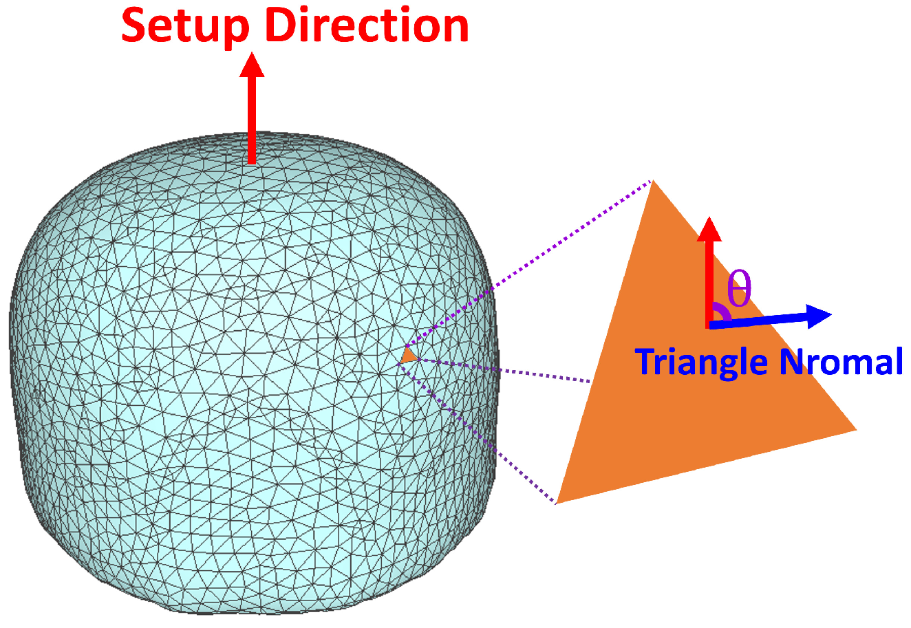
In five-axis CNC machining, to achieve compatibility between tool inclination and the geometric features of the triangular faces, ensuring tool accessibility and scallop height constraints, the original surface needs to be segmented into shallow (regions where the angle between the surface normal and the setup direction is small) and steep regions (regions where the angle is large). Continuing with the semi-ellipsoid model, we calculate the angle $\theta$ between the normal vector $\mathit{n}$ of each triangular face and the previously determined setup direction, as illustrated in Figure 4.

We first classify the triangular faces into steep and shallow categories based on a predefined threshold angle. The selection of this threshold is based on extensive industrial testing and practical experience; for instance, in the “Steep and Shallow Finishing” strategy of the commercial software PowerMill, users commonly adopt ${40}^{\circ }$ as the boundary angle, and this threshold has been verified as effective in actual machining processes. Therefore, we set the threshold to ${40}^{\circ }$. Faces with $\theta <{40}^{\circ }$ are classified as shallow regions (the top cap of the semi-ellipsoid), while those with $\theta \ge {40}^{\circ }$ are classified as steep regions (the side walls), as clearly distinguished by different colors in the “Shallow/Steep Division” step of Figure 2. After the initial classification, connected faces are merged to form continuous regions. However, this process may introduce two types of topological defects: (1) small isolated shallow sub-regions and (2) holes within shallow regions. To eliminate these defects, iterative processing steps are required.

In the iterative processing steps, for the shallow subregions, isolated branches with an area smaller than a set threshold are removed and merged into the steep region. For holes within the shallow region, boundary expansion is performed iteratively to gradually absorb adjacent surface segments. In each iteration, let the candidate triangle be denoted as f, the current shallow branch as R, and let the set of triangle surface segments that share at least one point with f be denoted as $E_f$. An adjacency measure can be established for each candidate surface segment:

$$\begin{array}{c}\hfill {\eta }_f={\displaystyle \frac{|E_f\cap R|}{|E_f|}}.\end{array}$$

(2)

When ${\eta }_f\ge 0.5$, f is merged into the current branch until no further expansion is possible, a complete and continuous segmentation of the machining regions is ultimately formed. It is worth noting that the segmentation algorithm may result in non-smooth region boundaries. However, since the subsequent path generation uses the iso-planar method (not contour offset method), which is not sensitive to boundary quality, this segmentation method is feasible.

3.3. Collision Detection on Triangular Mesh

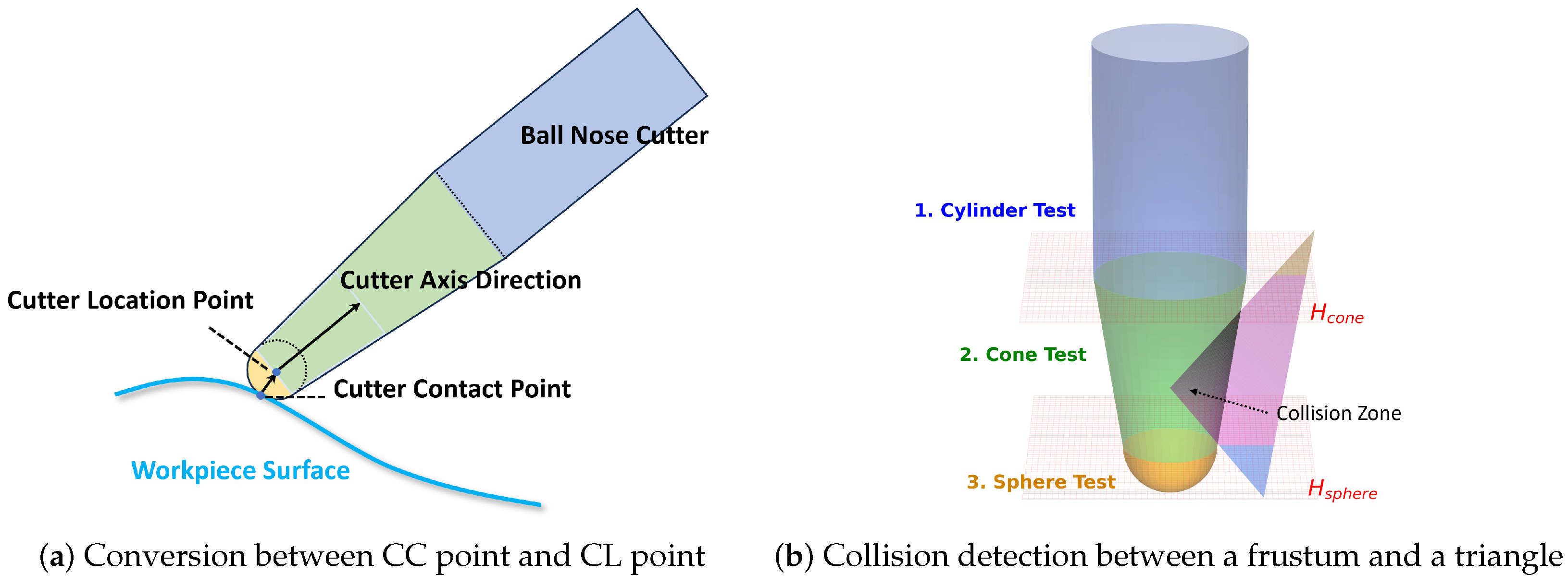
Collision-free machining is a fundamental requirement for CNC tool path planning. A mainstream method for collision detection involves discretizing the workpiece surface into triangular mesh vertices or point clouds [22,23], and determining accessibility by calculating the spatial relationship between sampling points and the tool axis. This method can be accelerated using hierarchical acceleration structures (e.g., octrees, OBB bounding boxes) [24,25], but may suffer from missed detection errors in high-curvature regions due to insufficient sampling density. In contrast, the method proposed in this paper detects collisions by calculating whether the triangular mesh intersects with the tool surface, achieving higher accuracy. The algorithm takes as input the triangular mesh model, cutter contact (CC) point coordinates, model surface normal vector, tool axis orientation, and tool geometric parameters. It automatically calculates the cutter location (CL) point and outputs a Boolean variable indicating the collision result. The CL point is determined by offsetting the CC point along the direction of the model surface normal vector by a distance equal to the tool radius.

Collision-free tool path generation with respect to the workpiece model is the most fundamental requirement in CNC machining. The collision detection algorithm proposed in this paper automatically calculates the tool position and outputs a Boolean variable indicating the collision result by inputting the triangular mesh model, CC point coordinates, model surface normal vectors, tool axis direction, and tool geometry parameters. The determination of the CL point is shown in Figure 5a. By offsetting the tool contact point along the model surface normal direction by the tool radius, the tool position can be obtained. Then, by decomposing the tool geometry, the collision detection problem is transformed into an intersection determination problem between quadratic surfaces and triangles.

The ball-end mill used in this study can be decomposed into a combination of three basic geometric bodies: a cylindrical section, a frustum of a cone, and a hemispherical cutter head. These geometric bodies can be described as the Boolean intersection of quadratic surfaces and half-spaces. The half-space is defined as the set of points in three-dimensional space that satisfy the linear inequality $\mathit{n}\mathit{x}+d\ge 0$ (where $\mathit{n}$ is the normal vector and d is the offset), which geometrically represents the boundary plane dividing the space into two infinite regions. Directly determining whether they collide with a triangle is challenging, but we can simplify the problem by first performing the intersection operation between the triangle and the half-space.

Taking the frustum of a cone as an example, let the region enclosed by the conical surface of the frustum’s side be denoted as $H_1$, the downward half-space cut by the plane of the upper base of the frustum be denoted as $H_2$, and the upward half-space cut by the plane of the lower base of the frustum be denoted as $H_3$. The interior of the frustum can then be expressed as $H_1\cap (H_2\cap H_3)$. Let the geometry of all points inside (including the boundary) of the triangle be denoted as T, and the collision detection can be reduced to determining the emptiness of the set $\Omega =(H_1\cap (H_2\cap H_3))\cap T$. Since the intersection operation satisfies the associative law, we have

$$\begin{array}{c}\hfill \Omega =H_1\cap ((H_2\cap H_3)\cap T).\end{array}$$

(3)

Therefore, we can first use the plane clipping algorithm to convert the triangle into a polygon P and then detect the surface intersection between P and $H_1$, as shown in Figure 5b. Specifically, following the framework in [26], the quadric surface $H_1$ is rigorously defined by the inequality:

$$f\left(\mathit{x}\right)={\mathit{x}}^T\mathbf{Q}\mathit{x}+{\mathbf{V}}^T\mathit{x}+c\le 0.$$

(4)

To ensure the completeness of collision detection, we systematically verify the intersection between the polygon P (lying on plane $\Pi$) and $H_1$ through four topological cases:

1.

Vertex Inclusion Test: If any vertex ${\mathit{v}}_i$ of P satisfies the quadric inequality, a collision is detected:

$$\exists {\mathit{v}}_i\in \mathrm{Vertices}\left(P\right),f\left({\mathit{v}}_i\right)\le 0.$$

(5)

2.

Edge Intersection Test: The intersection between the boundary edges of P and the quadric surface $\partial H_1$ is determined by solving the quadratic equation along each edge segment ${\mathit{e}}_{ij}={\mathit{v}}_i+t({\mathit{v}}_j-{\mathit{v}}_i)$. Real roots within $t\in [0,1]$ indicate a collision.

3.

Axis Intersection Test (for Cylinder/Frustum): The intersection curve $\gamma =\partial H_1\cap \Pi$ may be entirely contained within the interior of P without crossing any edges. For quadrics of revolution, this topological case is detected by checking if the intersection point ${\mathit{p}}_{axis}$ of the tool axis L and plane $\Pi$ lies within P:

$${\mathit{p}}_{axis}=L\cap \Pi ,{\mathit{p}}_{axis}\in P.$$

(6)

Note that for open curves (hyperbolas/parabolas), the Jordan Curve Theorem guarantees that if the interior intersection is non-empty, the curve must cross the polygon boundary (detected by Step 2). Thus, this step is specific to closed curves (ellipses).

4.

Center Projection Test (for Sphere): For a spherical tool component with center $\mathit{c}$ and radius R, the intersection region on $\Pi$ is a disk. A collision occurs if the orthogonal projection ${\mathit{p}}_{proj}$ of $\mathit{c}$ onto $\Pi$ falls within P and the distance condition is met:

$${\mathit{p}}_{proj}\in P\wedge \parallel \mathit{c}-{\mathit{p}}_{proj}\parallel \le R.$$

(7)

This rigorous approach guarantees algorithmic robustness by covering all topological configurations of surface–polygon intersections. The relevant pseudocode is shown in Algorithm 2.

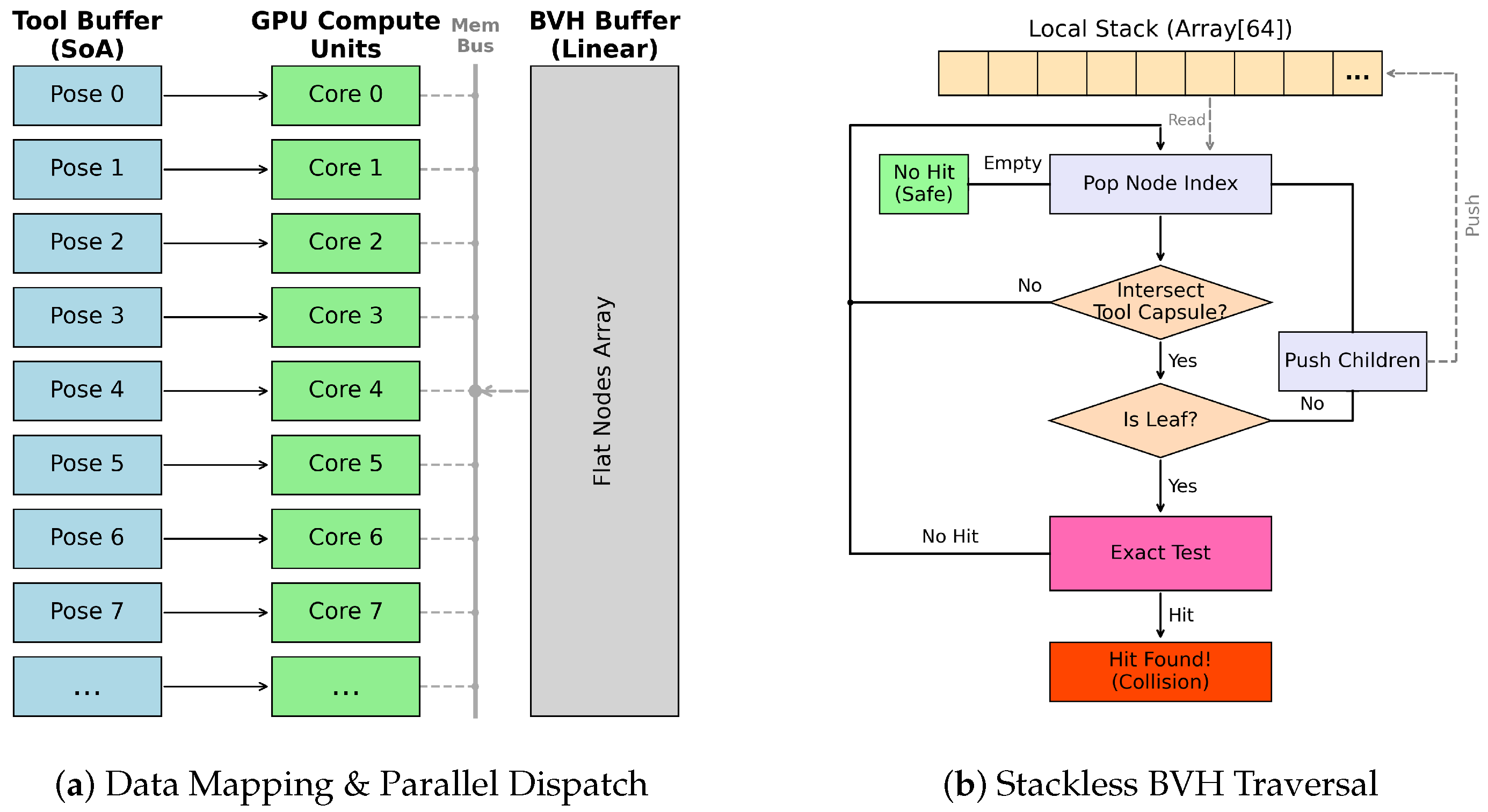
Due to the fact that precise surface representation in triangular mesh requires a large number of triangles, the collision detection method proposed in this paper runs slowly when executed serially on the CPU. However, since the collision detection tasks for different tool poses are independent, this process can be highly parallelized. To optimize spatial queries, the triangular mesh is first preprocessed into a Bounding Volume Hierarchy (BVH) on the host CPU. This structural construction is a one-time initialization task. The resulting tree is subsequently linearized into a contiguous memory block (Linear BVH) and transferred to the GPU. Figure 6a illustrates the memory layout, while Figure 6b depicts the flowchart of the parallel collision detection pipeline. The architecture consists of three stages corresponding to the compute shader logic:

• Data Mapping and Memory Layout: We utilize a Structure of Arrays (SoA) layout for the Tool Buffer and a linearized array for the BVH Buffer. The compute shader dispatch aligns the global invocation ID with the tool buffer index, enabling a one-to-one mapping where each GPU thread processes a unique tool pose independently.
• Stack-based BVH Traversal: To adapt to the GPU’s non-recursive execution model, we implement a stackless traversal algorithm. Each thread maintains a local array (size 64) acting as a software stack. The traversal loop performs broad-phase culling by testing the intersection between the tool’s bounding capsule and the BVH node’s AABB.
• Exact Geometry Test: Upon reaching a leaf node, we perform rigorous narrow-phase detection. As shown in the right panel of Figure 5b, the algorithm employs a “slicing” strategy. The target triangle is clipped by horizontal planes defined by the tool’s geometric junctions (cylinder-cone and cone-sphere interfaces). The resulting polygons are then tested against the corresponding analytic surfaces (cylinder, cone, and sphere) to ensure mathematical exactness.

Algorithm 2 GPU-Based Parallel Exact Collision Detection

Require: Triangle T, Tool Definition (Cylinder, Cone, Ball parameters)

Ensure: Collision Status

1: Transform vertices of T to Tool Coordinate System local frame   2: Initialize Polygon $P_0\leftarrow T$   3: // 1. Machine Shank Safety Check   4: $P_{shank}\leftarrow \mathrm{ClipPolygonUp}(P_0,H_{machine})$   5: if $P_{shank}$ is not empty then return COLLISION   6: end if   7: // 2. Cylinder Body Check   8: $P_{cyl}\leftarrow \mathrm{ClipPolygonUp}(P_0,H_{cone\_top})$   9: if $P_{cyl}$ is not empty then 10:       Project $P_{cyl}$ edges to $XY$ plane 11:       if Distance from origin to edges $<R_{cyl}$ then return COLLISION 12:       end if 13: end if 14: // 3. Cone Segment Check 15: $P_{cone}\leftarrow \mathrm{ClipPolygonDown}(\mathrm{ClipPolygonUp}(P_0,H_{cone\_bottom}),H_{cone\_top})$ 16: if $P_{cone}$ not empty then 17:       if Vertices or Edges violate cone inequality $x^2+y^2<k^2{z}^2$ then return COLLISION 18:       end if 19: end if 20: // 4. Ball Head Check 21: $P_{ball}\leftarrow \mathrm{ClipPolygonDown}(P_0,H_{cone\_bottom})$ 22: if $P_{ball}$ not empty then 23:       if Distance from $P_{ball}$ to ball center $<R_{ball}$ then return COLLISION 24:       end if 25: end if 26: return SAFE

Compared with the method of Bi et al. [27], our approach eliminates the need for rasterization pipelines. Instead, collision detection is processed directly within compute shaders, efficiently utilizing the GPU’s massive parallelism.

3.4. Path Segment Generation Based on Iso-Planar Method

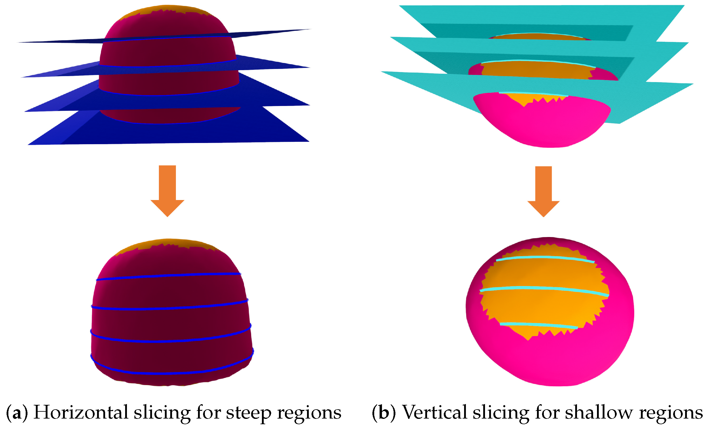
The goal of the algorithm in this section is to generate tool path segments within each region based on the results of shallow and steep boundary division. First, for each region, a set of parallel cross-sectional planes with the same normal vectors is generated (iso-planar method), and the intersection lines between the planes and the region surface are calculated. These intersection lines are referred to as contour lines. For the semi-ellipsoid model, different slicing strategies are applied to different regions. As shown in Figure 7a, the steep side walls are sliced by a set of horizontal planes (parallel to the XY plane), generating elliptical contour lines. Conversely, as shown in Figure 7b, the shallow top cap is sliced by a set of vertical planes (parallel to the YZ plane), generating arc-shaped contour lines. This differentiation ensures that the tool paths conform to the local geometry of the surface.

Then, the contour line is discretized into a set of points based on a pre-set atomic segment length $L_a$, and the points in the set are defined as atomic segments. Afterward, by performing reachability analysis (obstacle collision detection), tool cutter contact points that satisfy the continuous machining conditions within the same contour line are connected to form path segments. The algorithm in this section is similar to the one in [6], with the difference that, in this paper, different normal vectors for the cross-sectional planes are selected for different regions. The selection of the cross-sectional plane normal vectors follows a partitioning strategy: the steep region directly uses the machine clamping direction, while the shallow region is optimized and determined using the method described in Section 3.5.

It is important to note that a single cross-sectional plane does not necessarily result in just one contour line. The connection between atomic segments will be considered separately for unconnected contour lines. Additionally, since the regions after partitioning are no longer closed, the contour lines generated by the cross-sectional planes may not be closed either.

3.4.1. Accessibility Analysis

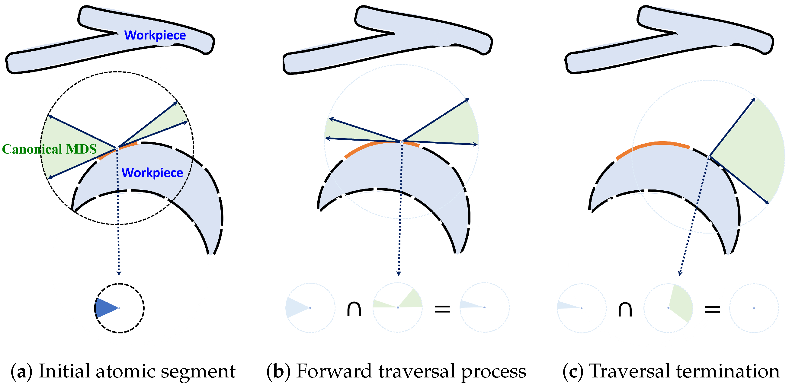
Based on the rational selection of iso-planar normals, this section constrains the tool axis direction within a two-dimensional plane perpendicular to the iso-planar normal. For the discretized atomic segments on the contour line, the Machinable Direction Range (MDR) is defined as the set of all tool directions that satisfy the collision-free condition. Since continuous machinable directions form a sector, the MDR actually consists of several continuous direction intervals, each called a Machinable Direction Sector (MDS), as shown in Figure 8. The largest MDS of an atomic segment is referred to as the canonical MDS of that point.

To efficiently solve the MDR, the algorithm in this section adopts a discretization sampling strategy: collision detection is performed at intervals of $5^{\circ }$ within the constraint direction domain. After marking the reachable directions, the MDS intervals are constructed based on connectivity. Subsequently, we use the forward and backward traversal algorithm from [6] to select directionally compatible MDSs (where the MDS intersection is non-empty) for stitching between adjacent atomic segments on the same contour line.

3.4.2. Forward and Backward Traversal Algorithm

The algorithm in this section aims to concatenate atomic segments on the same contour segment as much as possible while ensuring that the tool can move continuously along the path segment. The algorithm first requires an initial atomic segment to be input and one of its MDSs to be designated as the traversal MDS. Let the initial atomic segment be $A_i$ and record the current atomic segment index as $c\leftarrow i$. During the backward traversal process, let $e\leftarrow c+1$. If there exists an MDS in $A_e$ that overlaps with the traversal MDS of $A_c$ (i.e., their intersection is not empty), then $A_e$ can be merged, and that MDS is designated as the traversal MDS of $A_e$. Subsequently, let $c\leftarrow c+1$ for the next iteration. If no such MDS exists in $A_e$, the backward traversal terminates. At this point, the process restarts from the initial atomic segment and performs a forward traversal, letting $c\leftarrow i$ and $e\leftarrow c-1$, and iteratively merging atomic segments in the same manner, as shown in Figure 9. The set of atomic segments obtained through the forward and backward traversal algorithms is referred to as the tool path segment, with each atomic segment on the path segment having its unique traversal MDS.

Randomly selecting the starting atomic segment and traversing the MDS does not always yield good results. Path segments that can theoretically be merged are easily split by the algorithm. This paper adopts two heuristic strategies to optimize the greedy strategy from [6]: (1) When there are multiple MDSs that can overlap with the current traversed MDS for the next atomic segment, the one with the larger range is selected as the next atomic segment’s traversed MDS. (2) After completing the forward and backward traversal algorithm, the largest atomic segment representing the MDS among the remaining atomic segments is chosen as the starting point, and its canonical MDS is assigned as the starting MDS. In practice, these two strategies are sufficient to ensure the stability of the  Algorithm 3.

Algorithm 3 Heuristic Forward and Backward Traversal

Require: Contour Atomic Segments $\mathcal{A}=\{a_1,\dots ,a_n\}$

Ensure: Connected Path Segments $\mathcal{P}$

1: Initialize visited array $V\leftarrow {\left\{0\right\}}^n$   2: while exists unvisited segment in $\mathcal{A}$ do   3:       Select start segment $a_{start}$ with largest canonical MDS area   4:       $current\leftarrow a_{start}$, $Pat{h}_{curr}\leftarrow \left\{a_{start}\right\}$   5:       Mark $a_{start}$ as visited   6:       // Forward Traversal   7:       while neighbor $next$ of $current$ is unvisited AND feasible do   8:             $MDS\left(next\right)\leftarrow SelectMaxOverlapMDS\left(MDS\right(current),next)$   9:             Append $next$ to $Pat{h}_{curr}$, Mark $next$ visited 10:             $current\leftarrow next$ 11:       end while 12:       // Backward Traversal 13:       $current\leftarrow a_{start}$ 14:       while neighbor $prev$ of $current$ is unvisited AND feasible do 15:              $MDS\left(prev\right)\leftarrow SelectMaxOverlapMDS\left(MDS\right(current),prev)$ 16:              Prepend $prev$ to $Pat{h}_{curr}$, Mark $prev$ visited 17:              $current\leftarrow prev$ 18:       end while 19:       Add $Pat{h}_{curr}$ to $\mathcal{P}$ 20: end while 21: return $\mathcal{P}$

3.5. Optimal Machining Direction Selection for Shallow Regions

The algorithm in this section ensures the machinability of the shallow regions and improves the path continuity by optimizing the cross-sectional plane normal. For five-axis machines, given an atomic segment, the reachable directions at that point ideally form a hemisphere. Considering the collision-free constraint, the reachable direction domain is a subset of this hemisphere. After selecting a cross-sectional plane normal, the reachable direction is constrained to be perpendicular to the cross-sectional plane normal, which reduces the reachable direction domain of the atomic segment to a two-dimensional MDR. At this point, if the size of the canonical MDS of the atomic segment is 0, it indicates that the point on the surface is unmachinable under the constraint of this cross-sectional plane normal; conversely, if the canonical MDS area of the point is larger, it means the point has better reachability, which is favorable for generating path segments with better continuity.

Since the normal vectors of the surface segments in the shallow region are relatively consistent, we can restrict the candidate cross-sectional plane normals to planes orthogonal to the region’s average normal vector and evaluate each candidate normal through discretized sampling. Taking into account the balance between computational complexity and path accuracy, we generate a set of candidate directions at intervals of $5^{\circ }$ within the constraint plane and discretely sample atomic segments in the shallow region to compute their canonical MDS. Since machinability is a hard constraint, we first eliminate candidate directions where the canonical MDS of the atomic segment is 0, avoiding unmachinable cases. For the remaining directions, we calculate the average size of the canonical MDS of the discretely sampled atomic segments, and finally select the direction that maximizes this average value as the optimal cross-sectional plane normal for the shallow region. This strategy quantifies the impact of different directions on path continuity, enabling the optimal selection of machining directions. The subsequent tool path generation is then treated the same as in the steep regions.

3.6. Path Segment Connection Based on TSP

3.6.1. Path Segment Endpoint Distance Calculation

Before connecting different path segments, it is necessary to calculate the transfer path length required to connect the endpoints of different path segments and treat it as the distance between the path segment endpoints. In this paper, three types of relationships between path segment endpoints are defined: (1) same path; (2) straight-line transfer; and (3) tool-lift transfer.

For endpoints on the same path, the transfer path length is set to 0. For endpoints on different paths, feasibility of transfer is first evaluated by performing discrete collision detection along the line connecting the two endpoints, with the tool radius as the step size. Since determining the tool orientation at these discrete points requires the tool axis direction and model surface normal, and we desire smooth transfer of the tool orientation along the straight line, we need to interpolate the results to determine the tool orientation, even though there is no true model surface normal along the line. Spherical Linear Interpolation (Slerp) is a geometric method that provides a constant-speed shortest path along the great circle of a unit sphere, ensuring smooth rotational transitions. The corresponding directions at the endpoints are interpolated using Slerp to generate the required directions. This method ensures smooth transition by performing quaternion interpolation on the direction vectors at the endpoints. At the endpoints, the tool axis direction is selected as the geometric median direction representing the MDS, and the model surface normal is taken as the actual normal. If the collision detection is passed, the distance between the two endpoints is set to the straight-line distance.

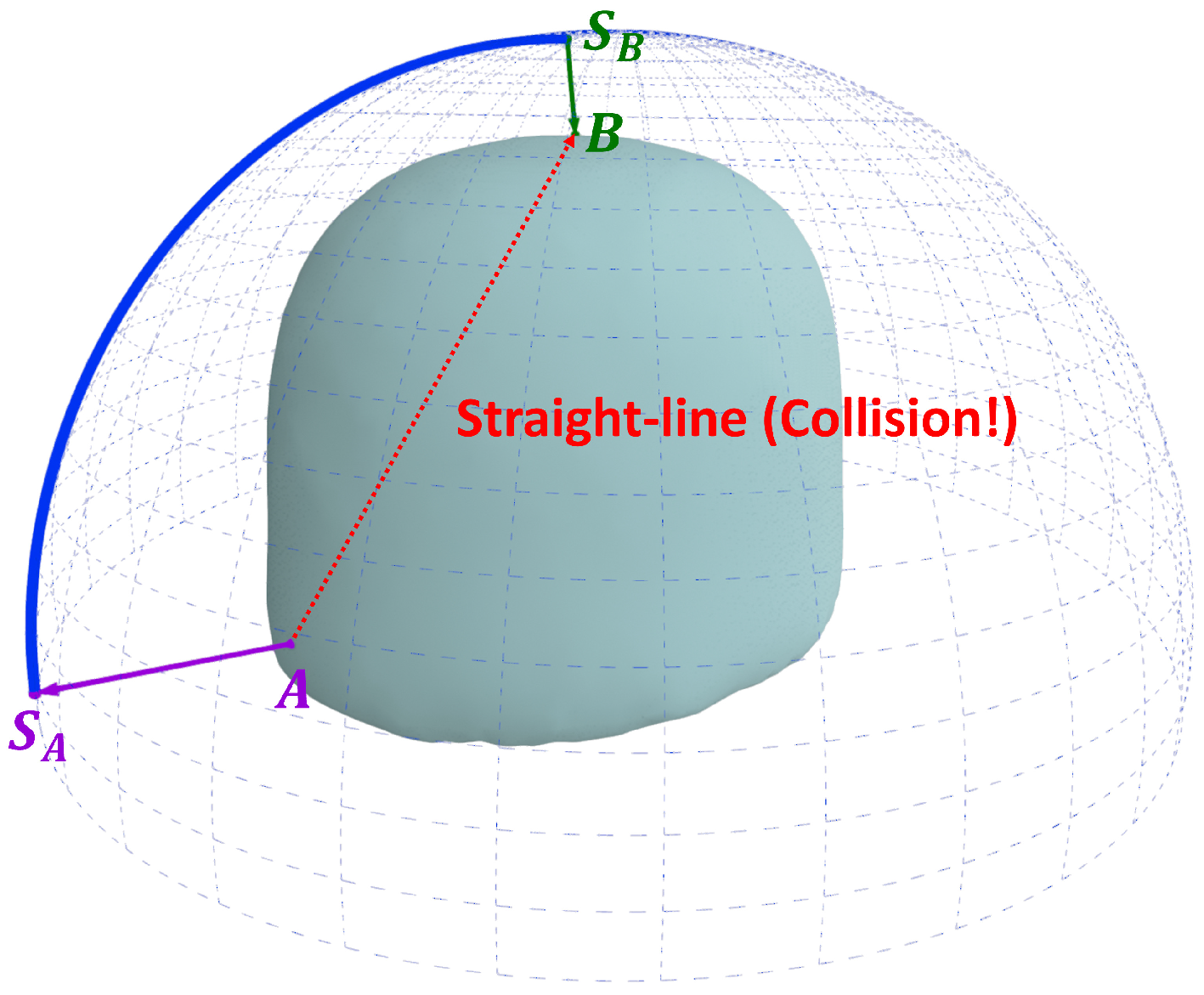
When the straight-line collision detection fails, the tool-lift transfer path length must be calculated. The construction of the tool-lift path is clearly illustrated in Figure 10. In this paper, a safety sphere with a radius slightly larger than the maximum bounding sphere of the model is constructed, centered at the fixture base center of the workpiece, ensuring that no collisions occur outside the sphere. Given two path segment endpoints A and B, they are projected along their respective tool axis directions to the safety sphere, resulting in projection points $S_a$ and $S_b$. The total transfer path length consists of three parts:

• The straight-line distance from the starting point A to its projection $S_a$ along the tool axis.
• The shortest distance along the geodesic (great circle arc) of the sphere from $S_a$ to $S_b$.
• The straight-line distance from $S_b$ to the endpoint B along the tool axis.

This logic guarantees a collision-free retract-transfer-plunge motion sequence.

3.6.2. Minimizing Transfer Path Length

This problem is essentially finding a path that traverses all segments with minimum transition cost. This optimization challenge is formally known as the Traveling Salesman Problem (TSP), an NP-hard problem in combinatorial optimization that seeks the shortest possible route visiting each node exactly once and returning to the origin. We construct a graph $G=(V,E)$ where V is the set of processable path segment endpoints. Two types of edges exist in E: fixed edges representing the path segments themselves (weight 0), and edges representing possible transfer moves between endpoints (weight calculated as in Section 3.1).

Existing research has applied TSP to tool path planning. For instance, Zhang et al. [6] modeled the path connection as a weighted complete graph and utilized a hybrid DFS/greedy solver to determine the traversal sequence. In contrast, our proposed approach explicitly establishes transformation rules for the open-path connection problem and employs the Christofides algorithm to guarantee a bounded approximation solution.

Acknowledging that the TSP is an NP-hard problem, we adopt a hybrid strategy based on the problem scale to balance solution quality and computational efficiency.

When the number of path segments is small ($n<50$), we employ an Integer Linear Programming (ILP) model to obtain the exact global optimal solution directly on the graph G. Let the binary variable $x_{ij}$ equal 1 if the edge $(i,j)$ is selected and 0 otherwise. The ILP model is formulated as follows:

$$\begin{array}{cc}\hfill min& \sum _{(i,j)\in E}{w}_{ij}{x}_{ij}\hfill \end{array}$$

(8)

$$\begin{array}{cc}\hfill \mathrm{s}.\mathrm{t}.& \sum _{j\in V,j\ne i}{x}_{ij}\le 2,\forall i\in V\hfill \end{array}$$

(9)

$$\begin{array}{cc}\hfill & \sum _{(i,j)\in E}{x}_{ij}=\left|V\right|-1\hfill \end{array}$$

(10)

$$\begin{array}{cc}\hfill & \sum _{i,j\in S,i<j}{x}_{ij}\le \left|S\right|-1,\forall S\subset V,S\ne \varnothing \hfill \end{array}$$

(11)

$$\begin{array}{cc}\hfill & x_{uv}=1,\forall (u,v)\in \mathrm{fixed}\mathrm{segments}\hfill \end{array}$$

(12)

The objective function (8) aims to minimize the total length of transfer moves. Constraint (9) restricts the degree of each node to at most 2, ensuring the solution is a path structure rather than a branching tree. Constraint (10) ensures that exactly $\left|V\right|-1$ edges are selected, which is the characteristic edge count of a spanning path. Constraint (11) is the Subtour Elimination Constraint (SEC) to prevent cycles. Constraint (12) enforces that all actual machining path segments must be included in the solution.

For larger scales ($n\ge 50$), we switch to the Christofides heuristic algorithm to avoid the exponential time complexity of ILP. However, since standard TSP solvers target Hamiltonian cycles without mandatory edge constraints, we apply a specific transformation to adapt our problem:

• Topology Transformation: To map the open-path problem to a closed-loop model, we introduce a dummy node O to construct an extended graph $G_1$ by connecting O to all original nodes with zero-weight edges. The optimal open path in G is thereby equivalent to the optimal Hamiltonian cycle in $G_1$.
• Weight Adjustment: To ensure the traversal of fixed machining segments (required edges), we employ a penalty-based weight adjustment. Let M be the maximum edge weight. By assigning a weight $N=-(m-n)M$ (where m is the node count and n is the required edge count) to all required edges, we mathematically guarantee that any optimal cycle must include all required edges [6]. A positive offset is subsequently added to ensure non-negative weights for the solver.

Upon this transformed model, the Christofides algorithm provides a 1.5 approximation with a polynomial time complexity of $O\left(n^3\right)$. This effectively meets the engineering needs of this paper.

3.7. Adaptive Path Refinement

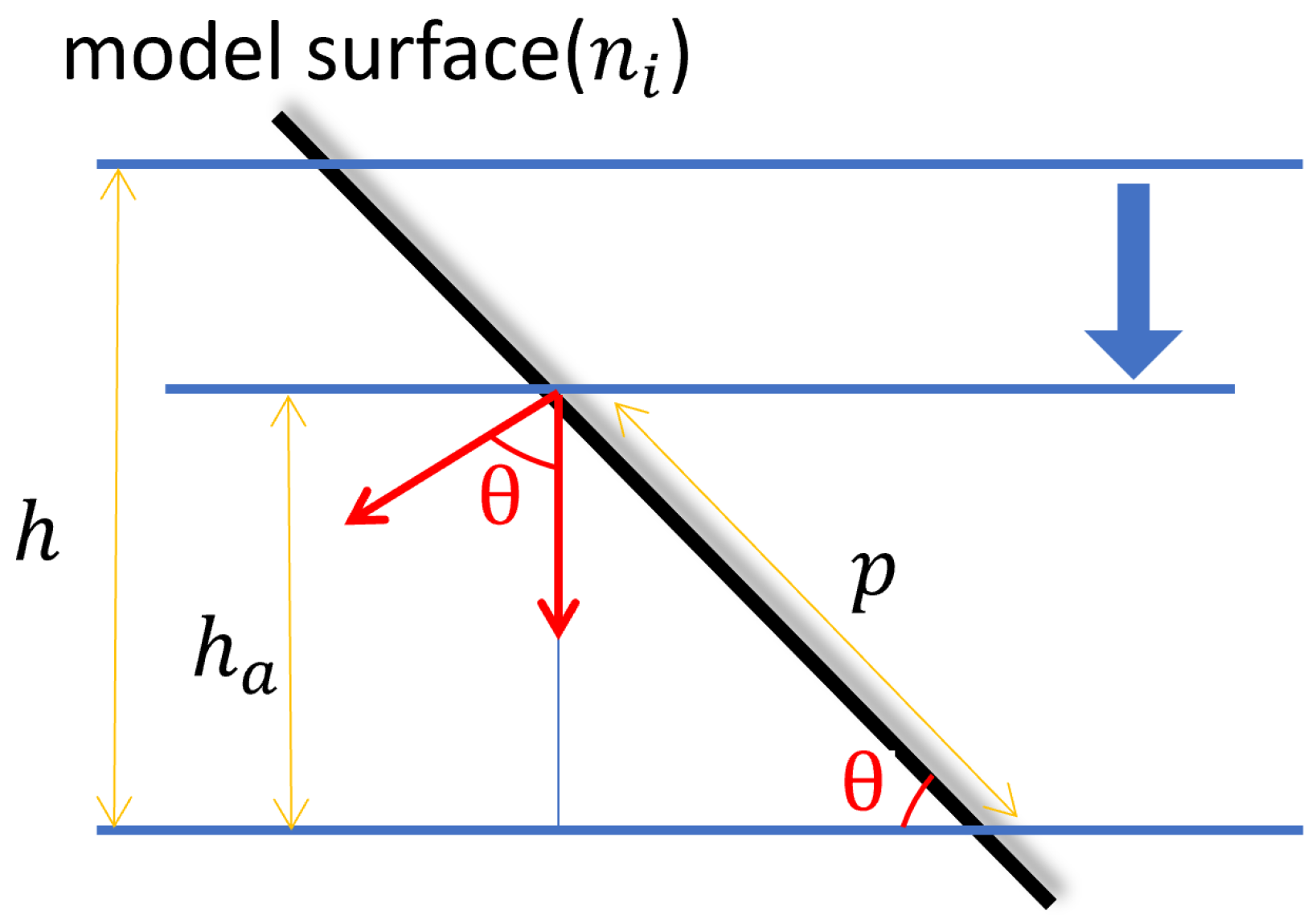
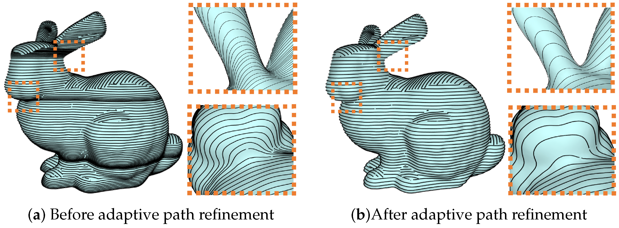
In CNC tool path planning, the actual path interval constraint is essentially the geodesic distance between adjacent tool paths on the model surface, which is approximated by the spatial distance between iso-planes in existing methods. For regions where the angle between the surface normal and the setup direction is significantly large (e.g., steep side walls of the semi-ellipsoid), this approximation fails. Figure 11 demonstrates this geometric relationship. With a constant iso-plane interval h, the actual geodesic interval on the surface becomes approximately $h/sin{\theta }_i$, where ${\theta }_i$ is the angle between the iso-plane normal $\mathit{m}$ and the surface normal ${\mathit{n}}_i$.

Therefore, this paper proposes a dynamic interval adjustment method based on geometric projection: Let the preset desired interval be h, the current iso-plane normal be $\mathit{m}$, the set of indices of the triangular faces intersected by the iso-plane be T, and the normals of the faces be ${\mathit{n}}_i,i\in T$. The adjusted interval for the next iso-plane $h_a$ should be

$$\begin{array}{c}\hfill h_a=h·\underset{i\in T}{min}\{sin{\theta }_i\},{\theta }_i=arccos(\mathit{m}·{\mathit{n}}_i).\end{array}$$

(13)

By reducing the plane interval $h_a$ by the factor $sin{\theta }_i$, we effectively compensate for the projection distortion, ensuring that the actual path interval p on the model surface remains close to the desired value h.

In this way, when the angle between the iso-plane normal (the opposite direction of the setup direction) and the face normal is close to perpendicular, the sine value is close to one, and the interval is close to the preset h, whereas when the angle is small, the sine value decreases, thereby reducing the interval to ensure that the path interval projection on the model surface remains reasonable. An example is shown in Figure 12.

4. Experimental Results and Analysis

4.1. Parameter Settings

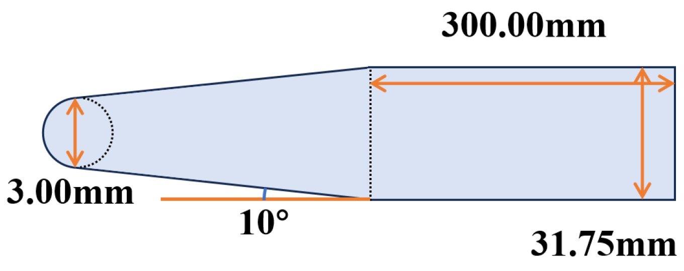
We select six models for testing. The experiments first normalize the models to a unified size: keeping the original model’s bounding box length–width–height ratio unchanged, the maximum edge length is normalized to 30cm to unify the model scale. The specific dimensions and number of triangular faces of the test models are detailed in

Table 1. Basic Information of Test Models.

Model Name	Size (cm)	Number of Faces
Bunny	$23.15\times 30.00\times 29.59$	59,694
Beetle	$12.16\times 30.00\times 10.33$	7558
Kitten	$19.53\times 17.78\times 30.00$	6356
Bone	$11.87\times 10.06\times 30.00$	9328
Twirl	$25.91\times 22.18\times 30.00$	10,398
Hand	$22.45\times 10.45\times 30.00$	7406

. The tool used is a ball-end mill with the cross-section shown in Figure 13, and its geometric parameters are set as follows: tool head diameter of 3.0 mm, conical section angle $\alpha$, cylindrical section diameter of 3.175 cm, length of 30 cm; atomic segment length $L=1$ mm, discretization angle fixed at $\theta =5^{\circ }$, and safety sphere radius set to 35 cm.

The experiment is implemented in C++17, compiled with Microsoft Visual Studio 2022 (MSVC 19.42) compilation environment, and the collision detection module utilizes Vulkan 1.0 API [28] for GPU acceleration. All tests are run on the same experimental platform, with the operating system being Windows 11 and hardware configuration as follows: Intel Core i9-13900KF processor, NVIDIA GeForce RTX 4090 graphics card.

4.2. GPU Acceleration Performance Analysis

To quantitatively evaluate the GPU acceleration effect, this experiment randomly samples 10,000 points on the model surface as tool contact points and generates random tool poses for each contact point, randomly determining the tool axis direction and recording the corresponding surface normal vectors. This method constructs 10,000 sets of test data to ensure a robust performance metric. The tests are run on the same hardware platform. For the CPU baseline, we implement a multi-threaded version using the C++ standard threading library, spawning threads equal to the number of logical processors (32 threads) to fully utilize the available computational resources of the Intel i9 processor. This is compared against the GPU-accelerated version implemented in Vulkan. The computation time and acceleration ratios are shown in

Table 2. Performance comparison between CPU (Multi-threaded) and GPU (Vulkan) for 10,000 collision checks.

Model	CPU Time (ms)	GPU Time (ms)	×Speedup
Bunny	12,802.70	130.47	98.13
Beetle	2539.74	18.06	140.63
Kitten	4136.00	19.76	209.31
Bone	5309.78	43.45	122.20
Twirl	8239.82	38.16	215.93
Hand	3311.19	30.45	108.74

.

It can be seen that, even compared to the multi-threaded CPU implementation, the GPU parallel algorithm computational efficiency has improved by a factor of 98. This significant speedup is attributed to the massive parallelism of the GPU and the efficient stack-based BVH traversal which minimizes memory latency. For the Bunny model, the GPU completes the collision detection for all 10,000 poses in 131 ms, whereas the CPU multi-threaded implementation requires 12 s. The results demonstrate that the proposed method meets the real-time requirements for complex path planning tasks.

To further assess the scalability of the proposed method for industrial-scale applications, we conducted a stress test on a high-resolution mesh exceeding 900k faces. By applying midpoint subdivision—a geometric algorithm that recursively divides each triangle into four smaller ones by connecting the edge midpoints—twice to the Bunny model, we generated a dense mesh containing 955,104 triangular faces, representing a 16-fold increase in geometric complexity. For this large-scale dataset, the BVH construction on the host CPU was completed in 550 ms. In terms of memory efficiency, the total GPU memory consumption (including Vertex Buffer, Index Buffer, and Linear BVH nodes) was recorded at approximately 58.3 MB. The parallel collision detection for 100,000 random queries was executed in 574 ms. These results demonstrate that the algorithm maintains high throughput and reasonable resource usage even when processing geometrically complex models.

4.3. Tool Path Result Analysis

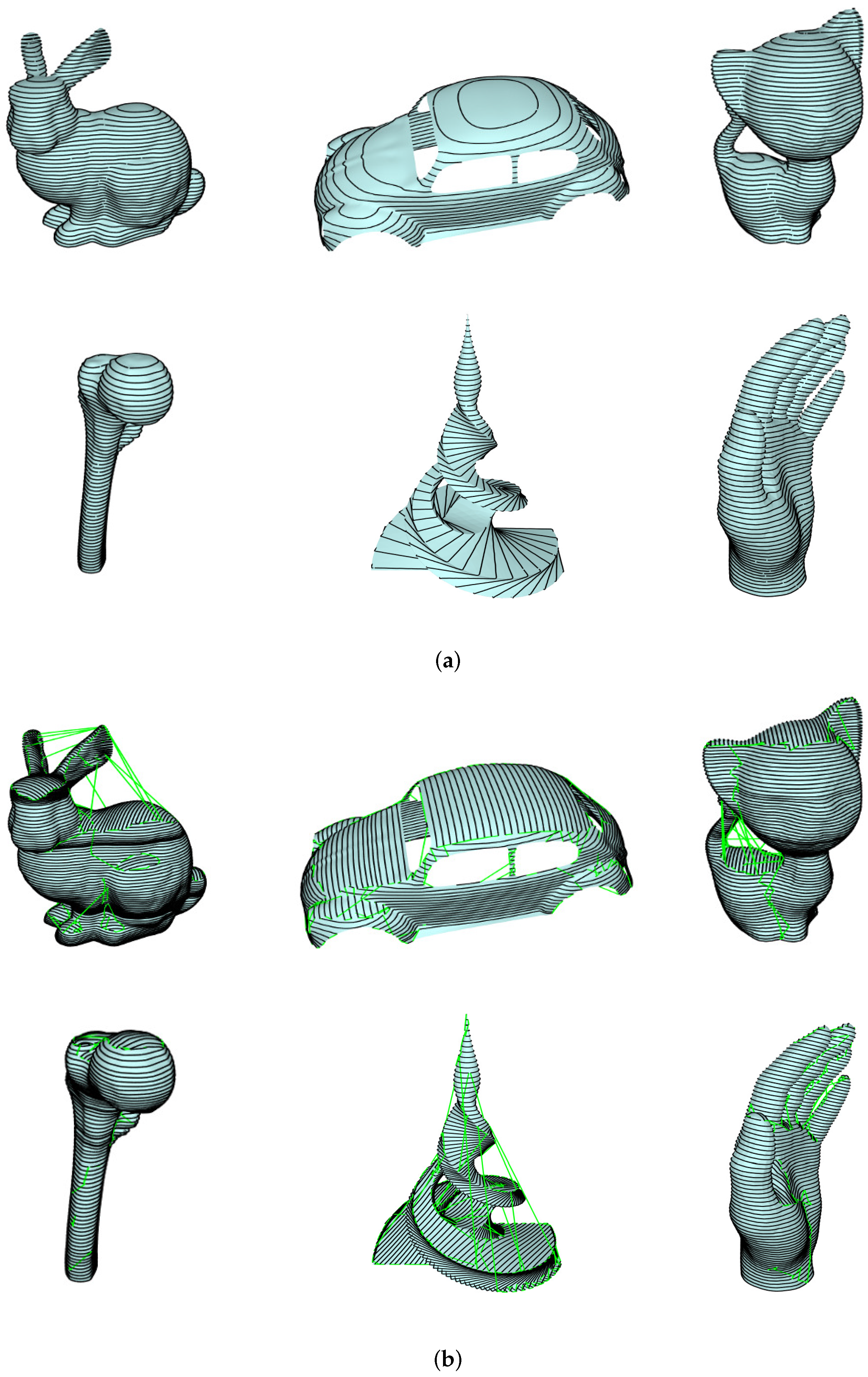
To visually demonstrate the algorithm’s effectiveness, the initial toolpath interval is fixed at 5mm, and the simulated path results are shown in Figure 14 (the black line represents the cutting path, and the green line represents the straight-line transfer path). To better display the cutting tool path, the tool lifting/landing lines and fast-moving lines are not shown. Since a five-axis machine can also complete tool paths originally planned for a four-axis machine, this paper also replicates the four-axis wrapping machining method from reference [6] as a comparison. The experimental results show that the tool path generated by the proposed algorithm can uniformly cover flat regions, effectively ensuring the surface quality of the machining.

It is noteworthy that the collision detection method in reference [6] has limitations: it only detects collisions within the same cross-sectional plane and therefore may lead to overcutting issues in practical machining. Specifically, when the angle between the tool contact normal vector and the assembly direction is less than ${10}^{\circ }$ (depending on the angle of the generatrix of the frustum), this issue becomes particularly significant due to the tool’s geometric parameters. The collision detection method used in this paper can more accurately identify potential collisions in the entire space, which causes some paths in the four-axis method to be automatically eliminated due to collision risks. This results in the formation of blind areas on the machining surface.

For the machining areas on the model surface with the normal direction pointing downward, the adaptive tool path refinement of this algorithm is highly effective. As shown in Figure 15, compared with the fixed-interval tool path planning, the tool path density in the downward areas is significantly increased after adopting the adaptive refinement strategy, while the path intervals remain uniformly stable.

4.4. Scallop Height Analysis

In CNC machining, the scallop height requirement directly determines the final quality of the machined surface. Therefore, this section first needs to determine the optimal initial path interval based on the given scallop height constraint. The theoretical basis for this calculation relies on the Scallop Metric proposed by Zou [29]. The scallop height calculation is based on a 2D cross-sectional approximation. Assuming a cutter contact point $p_1$, a plane is created perpendicular to the feed direction. On this plane, the tool projection forms a circular arc with radius r, and the local workpiece surface is approximated by its osculating circle with radius R. The scallop height $h_s$ can be expressed by the second-order approximation equation:

$$h_s={\displaystyle \frac{R+r}{8Rr}}\parallel p_2-p_1{\parallel }^2+O(\parallel p_2-p_1{\parallel }^3)$$

(14)

where $\parallel p_2-p_1\parallel$ represents the side step (path interval). The normal curvature ${\kappa }_t$, which is the reciprocal of the radius R, is introduced, i.e., ${\kappa }_t=1/R$. The normal curvature can be calculated via the curvature tensor ${\mathbf{T}}_c$ as

$${\kappa }_t={\mathbf{u}}_t^T{\mathbf{T}}_c{\mathbf{u}}_t,{\mathbf{T}}_c={\kappa }_1{\mathbf{u}}_1{\mathbf{u}}_1^T+{\kappa }_2{\mathbf{u}}_2{\mathbf{u}}_2^T$$

(15)

where ${\mathbf{u}}_t$ is the tangent direction orthogonal to the feed direction, ${\kappa }_1,{\kappa }_2$ are principal curvatures, and ${\mathbf{u}}_1,{\mathbf{u}}_2$ are principal directions. Substituting ${\kappa }_t$ into the scallop height formula and defining a tool tensor ${\mathbf{T}}_r$ as a diagonal matrix with elements $1/r$, the formula can be reformulated as

$$h_s\approx {\displaystyle \frac{1}{8}}({\mathbf{u}}_t^T{\mathbf{T}}_c{\mathbf{u}}_t+{\displaystyle \frac{1}{r}}){\parallel p_2-p_1\parallel }^2={(p_2-p_1)}^T{\displaystyle \frac{{\mathbf{T}}_c+{\mathbf{T}}_r}{8}}(p_2-p_1)$$

(16)

Zou [29] proposed the Scallop Metric ${\mathbf{T}}_s$ to simplify this expression:

$${\mathbf{T}}_s={\displaystyle \frac{{\mathbf{T}}_c+{\mathbf{T}}_r}{8}}$$

(17)

Under this metric, the scallop height is simplified to a quadratic form:

$$h_s\approx {(p_2-p_1)}^T{\mathbf{T}}_s(p_2-p_1)$$

(18)

Consequently, generating iso-scallop paths is equivalent to planning paths with constant geodesic distance under the metric ${\mathbf{T}}_s$.

Based on this theory, we can derive the formula to calculate the interval h (corresponding to $\parallel p_2-p_1\parallel$) under a given scallop height requirement s (corresponding to $h_s$) [8]:

$$\begin{array}{c}\hfill h=\alpha \sqrt{{\displaystyle \frac{8Rrs}{R+r}}}.\end{array}$$

(19)

Here, h is the obtained initial path interval, R is the minimum curvature radius of the model surface, r is the tool radius, s is the given scallop height, and $\alpha$ is a correction factor. The reason for introducing the correction factor $\alpha$ is that in the transition junction between shallow and steep regions, the actual path interval may locally increase, leading to scallop heights exceeding the design requirements. By introducing the correction factor, it can be ensured that the scallop height constraint is met under the most unfavorable conditions. In the experiments of this paper, $\alpha$ is taken as 0.9. Additionally, the tool path in the shallow region can be slightly extended to further eliminate path interval anomalies at the junction.

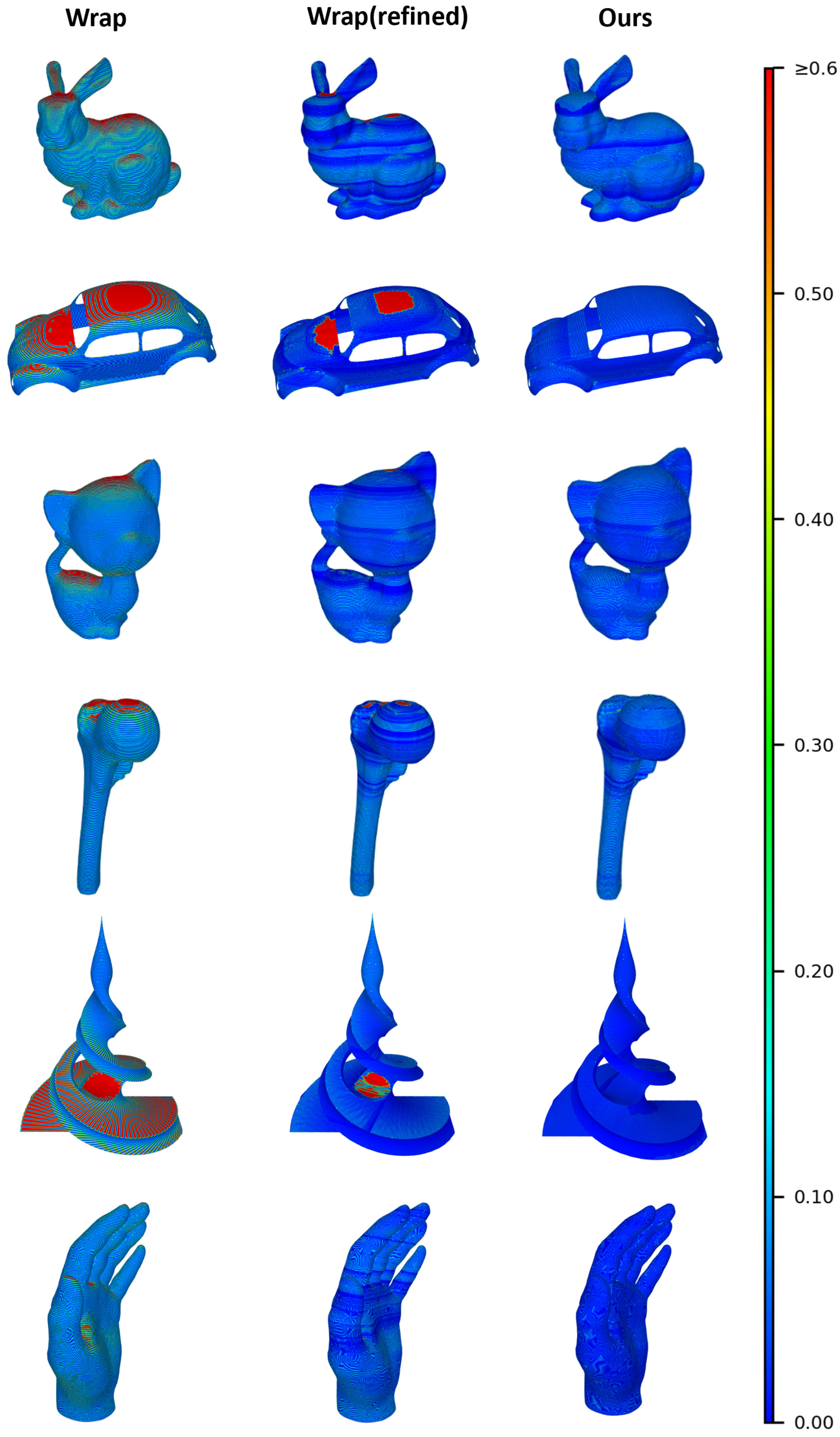
Under the conditions of a preset scallop height of 0.6mm and a scallop allowance of 2 mm before machining, the simulated scallop height results are shown in Figure 15. Among them, the maximum scallop heights for the Bunny, Beetle, Kitten, Twirl and Hand models are 0.58 mm, 0.53 mm, 0.48 mm, 0.53 mm and 0.58 mm, respectively, which meet the preset scallop height constraints. As shown in

Table 3. Comparison of Machining Quality Evaluation Indicators (S.-H. refers to scallop-height, bold fonts mean best values of the column).

Method	Model	Maximum	Average	RMS	Unprocessed	Path
	Name	S.-H. (mm)	S.-H. (mm)	S.-H. (mm)	Ratio (%)	Length ($\times {\mathbf{10}}^{\mathbf{4}}$mm)
Proposed Method	Bunny	0.58	0.05	0.07	0.00%	16.55
	Beetle	0.53	0.03	0.05	0.00%	5.59
	Kitten	0.48	0.04	0.06	0.00%	11.92
	Bone	2.00	0.05	0.05	0.06%	4.60
	Twirl	0.53	0.02	0.03	0.00%	12.06
	Hand	0.58	0.03	0.04	0.00%	8.27
Four-axis Method [5]	Bunny	2.00	0.25	0.51	5.53%	8.06
	Beetle	2.00	0.34	0.72	12.16%	2.87
	Kitten	2.00	0.18	0.41	3.49%	7.09
	Bone	2.00	0.18	0.40	3.43%	2.65
	Twirl	2.00	0.44	0.80	14.75%	2.42
	Hand	2.00	0.13	0.27	1.24%	4.27
Refinement of Method [5]	Bunny	2.00	0.06	0.20	0.88%	19.78
	Beetle	2.00	0.12	0.44	4.72%	7.30
	Kitten	2.00	0.05	0.11	0.17%	13.81
	Bone	2.00	0.07	0.17	0.53%	5.03
	Twirl	2.00	0.05	0.21	1.03%	8.08
	Hand	2.00	0.05	0.09	0.06%	6.28

, this paper’s method can cover the entire model’s machining, while the four-axis wrapping machining method [6] has significant unmachined areas and does not meet the high-precision machining requirements. If the four-axis wrapping machining method is further refined to make its average error close to that of this paper’s method, the generated path length is significantly longer than that of this paper’s method, and there are still unmachined areas. This indicates that the four-axis wrapping machining method has inherent defects for some models, further demonstrating the effectiveness of the method presented in this paper.

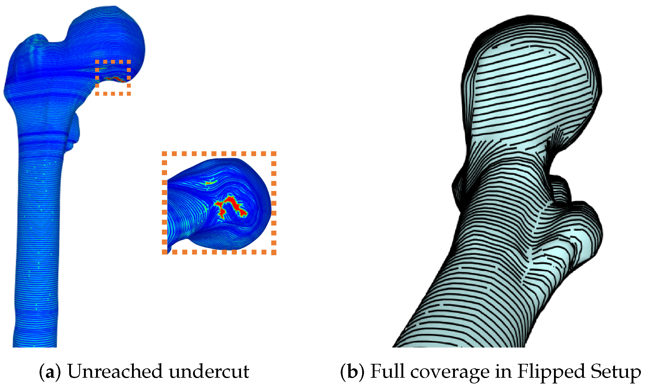
However, the reachability of single-setup machining is physically constrained by the setup direction. Specifically, any surface region where the angle between the surface normal and the setup direction (Z-axis) exceeds ${90}^{\circ }$ forms an undercut that is accessible only through re-fixturing. Although utilizing kinematic chains with higher degrees of freedom (e.g., 6-axis serial robots) could effectively bypass this limitation, such systems typically suffer from low structural stiffness, making them unsuitable for high-precision machining tasks. Consequently, standard 5-axis CNC machines—preferred for their rigidity—must rely on multi-setup strategies to address these geometric constraints. For example, the Bone model has an inward concave area with downward-facing normals (undercuts), which cannot be machined by five-axis machining under the current setup direction, resulting in the unmachined area shown in Figure 16a, with an area ratio of about 0.06%. The proposed method will significantly reduce these machining blind spots through adaptive refinement. For the extremely small unmachined areas, a multi-setup strategy is proposed. As illustrated in Figure 16b, by performing a flip-fixturing operation (re-orienting the workpiece by ${180}^{\circ }$), the previously occluded regions become up-facing and can be fully machined.

4.5. Comparison with Commercial Software UG

Since the method in [6] has been proven to be superior to Autodesk Fusion 360, we did not conduct further comparison with this commercial software.

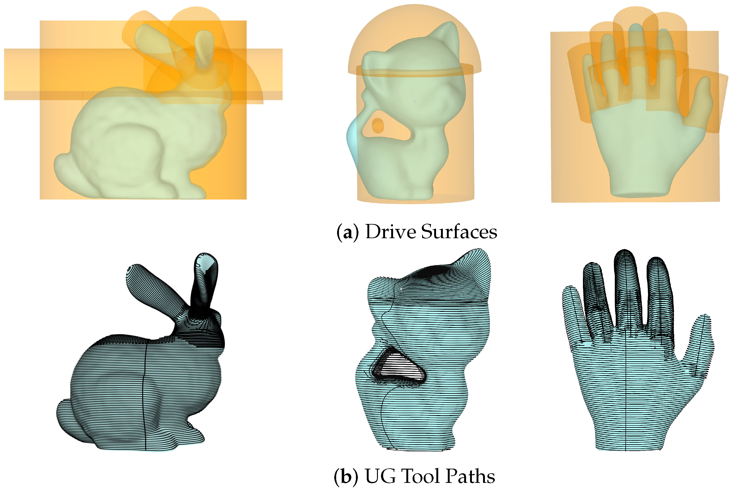
For UG, the commonly used variable axis contour milling strategy is adopted, and its workflow is as follows: (1) construct a reasonable drive surface; (2) generate a continuous tool path on the drive surface; and (3) project the generated tool path along the normal vector of the drive surface onto the target model to obtain the final machining tool path. From the above description, it can be concluded that the appropriate configuration of the drive surface is critical to the machining. From the perspective of Computer-Aided Manufacturing (CAM), this paper does not involve the fine design of the drive surface (see Figure 17a), but only uses the commonly used cylindrical or spherical surface for tool path generation.

Experimental results show that when using standard primitive drive surfaces (e.g., cylinder or sphere), there are still machining blind spots (see Figure 17b). It is important to acknowledge that experienced users can certainly generate valid, high-quality tool paths in Siemens NX by meticulously designing complex auxiliary drive surfaces and utilizing advanced axis control strategies. However, this process heavily relies on the user’s expertise and involves labor-intensive manual interactions within the CAD module. In contrast, the primary advantage of our proposed method lies in its high degree of automation. It eliminates the need for complex manual drive surface construction and achieves one-step generation of collision-free machining tool paths, making it accessible even for users without extensive CAM expertise. Quantitative comparisons are listed in

Table 4. Comparison between UG and Proposed Method on Different Models.

Model	UG			Proposed Method
	Retraction	Path Length ( $\times {\mathbf{10}}^{\mathbf{4}}$ )	Time	Retraction	Path Length ( $\times {\mathbf{10}}^{\mathbf{4}}$ )	Time
Bunny	127	20.35	≈1.3 h	42	16.55	21.43 min
Kitten	56	7.20	≈0.5 h	2	11.92	1.68 min
Hand	263	14.74	≈1.8 h	0	8.27	5.63 min

. The results indicate that our method significantly outperforms the simple manual UG workflow in terms of planning time and the number of retractions, validating its efficiency and robustness.

4.6. Comparison with Iso-Scallop Method

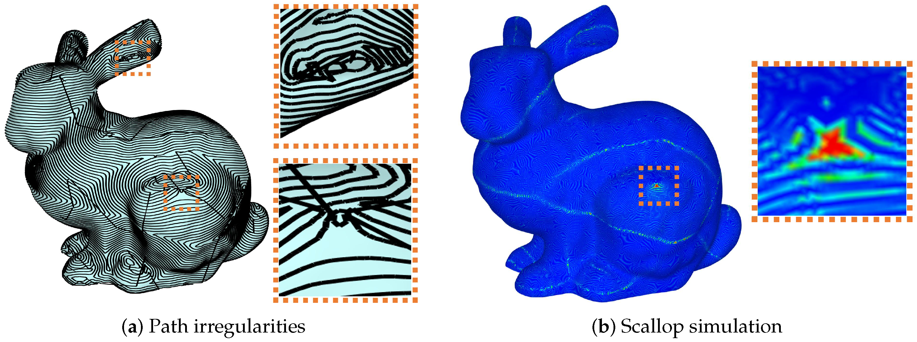
To evaluate the proposed method, we compared it with iso-scallop height methods for triangular meshes [3,30], which typically employ the heat method. The statistical results of the iso-scallop machining simulation are: Average S-H 0.03 mm, RMS S-H 0.04 mm, and Path length 20.71 $\times {10}^4$ mm. The generated tool path is shown in Figure 18a. The data indicate that although the iso-scallop method results in slightly longer tool paths than the proposed method, it achieves lower average and RMS scallop heights.

However, the iso-scallop method suffers from significant robustness issues. A key limitation is the sensitivity to mesh quality. Engineering models often contain ill-shaped triangles, characterized by extremely small areas or large aspect ratios. These irregular elements severely affect the accuracy of discrete curvature calculations. Since iso-scallop methods rely on these curvature values, calculation errors lead to inaccuracies in path generation. As a result, the tool paths may exhibit severe kinks and deviations, as shown in Figure 18a. Moreover, the simulation in Figure 18b indicates that these path deviations can result in scallop heights that exceed the specified constraints.

In contrast, the iso-planar method used in this study relies on cross-sectional slicing. This approach depends on geometric intersection rather than local differential properties, making it less sensitive to mesh topology. Consequently, it can generate smooth and collision-free paths even for meshes with lower quality. Therefore, for the automated machining of general triangular meshes, the iso-planar method demonstrates significantly higher robustness and practicality compared to current iso-scallop approaches. This is also one of the primary reasons why recent state-of-the-art research on triangular meshes [6] continues to employ the iso-planar method.

4.7. Physical Machining Verification

To further validate the detailed surface quality and the feasibility of the generated tool paths, we conducted physical cutting experiments on a compact five-axis machining center.

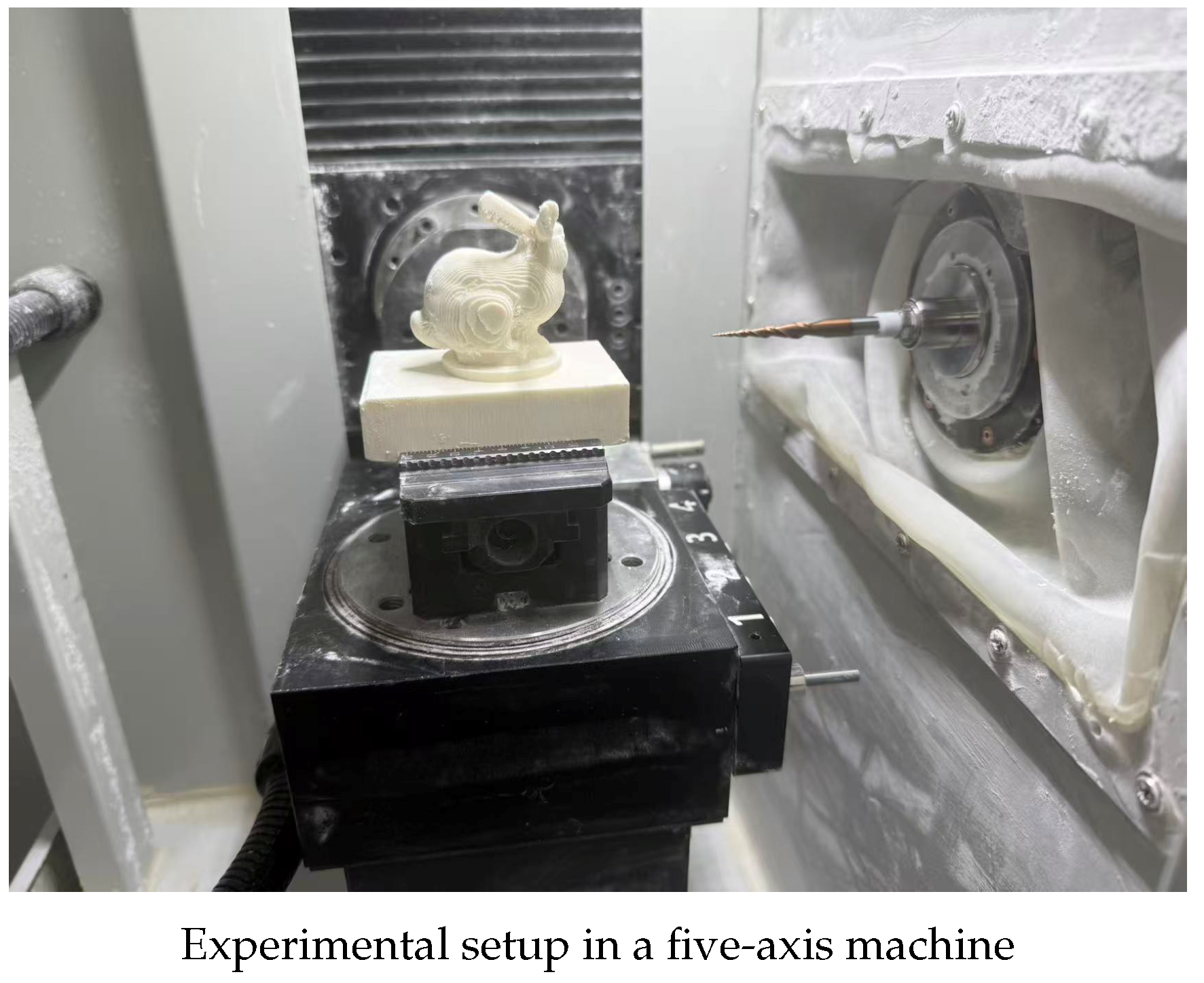
First, regarding the machining environment configuration: As shown in Figure 19, the equipment used in the experiment is a self-developed 5-axis desktop CNC machining center (dimensions: 800 mm in length, 530 mm in width, and 790 mm in height). The CNC system employed is independently developed by our team based on the open-source LinuxCNC system. Figure 19 illustrates the workpiece fixed on the machine table after rough machining, ready for the finishing process. It is important to note that, to adapt to the limitations of the experimental environment, both the model and the generated tool paths were scaled down to 1/10 of their original size for the physical machining trials. The cutting tool used was a tungsten steel tapered ball-end cutter (total length: 75 mm, tip diameter: 0.3 mm, half cone angle: ${10}^{\circ }$). The spindle speed was set to 16,000 r/min. Given that nylon is softer compared to metals, cutting fluid was not employed—instead, an air-blow cooling method was implemented to maintain process stability. The feedrate limit was set to 3000 mm/min, and the acceleration limit for each axis was set to 800 mm/s². Notably, the tool paths generated by UG are unmachinable, and thus, we only performed machining using the tool paths derived from our method and those from the state-of-the-art academic approach [6].

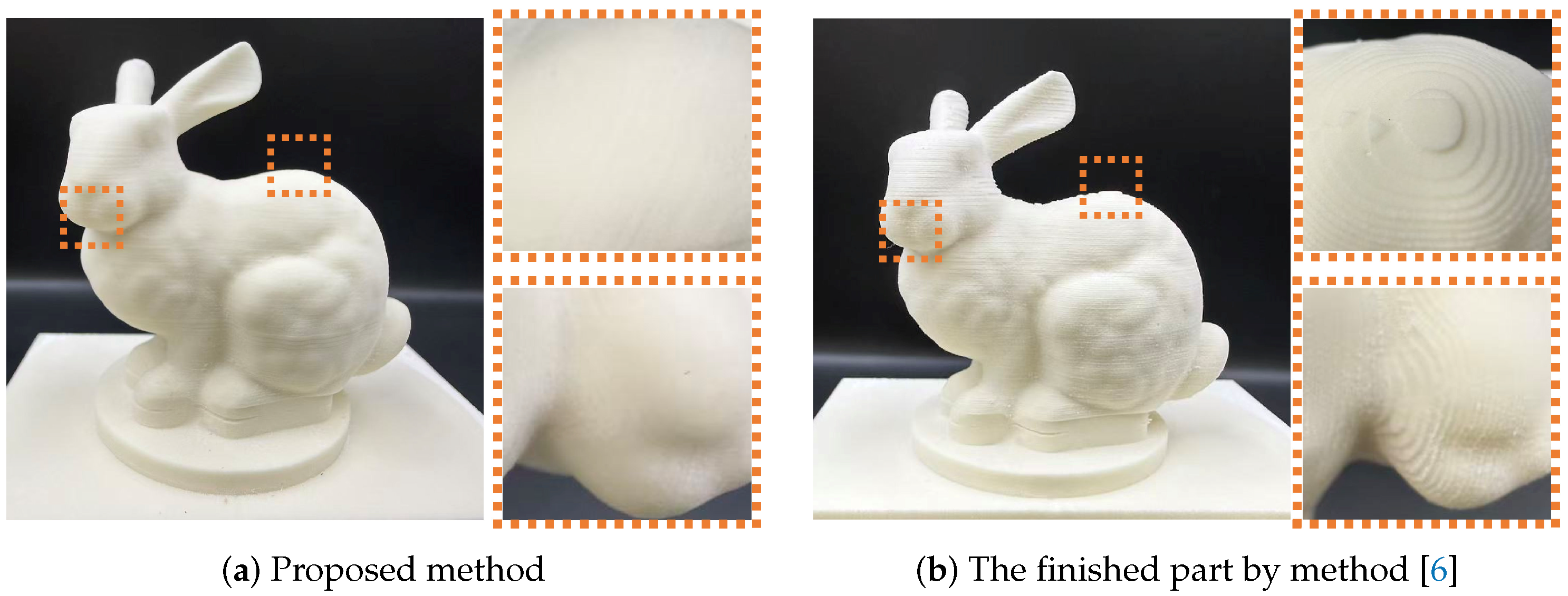
For the verification object, we selected the Bunny model, which contains both steep curvature changes and flat regions. We specifically compared the physical machining results of our proposed method against the wrapping method from Reference [6]. As clearly observed in Figure 20b, the method from [6] produces excessive scallop heights in the flat regions (the distinct step-like marks on the back of the bunny), which fails to meet the surface quality requirements. This confirms our theoretical analysis that fixed-direction wrapping paths degenerate in shallow areas. In contrast, the part machined using our method (Figure 20a) exhibits a uniform surface finish across both steep and shallow regions, effectively validating the advantage of our automated segmentation and adaptive path refinement.

5. Conclusions

This paper presents an integrated machining method for complete models, whose primary contribution lies in its ability to fully leverage the capabilities of 5-axis machine tools compared to conventional wrapping-based machining approaches. By generating tool paths within shallow regions, the proposed method effectively avoids excessively long paths and redundant machining.

The proposed method offers distinct advantages over existing strategies. Compared to 3+2-axis machining based on surface segmentation, our wrapping-based approach avoids the residual material defects at patch junctions, thereby ensuring superior surface continuity. Furthermore, unlike current state-of-the-art wrapping methods—both in academia (e.g., [6]) and commercial software (e.g., Siemens NX [20])—which often fail to process complex geometries without leaving blind zones, our method achieves full automation in eliminating these unmachined areas. This characteristic makes it particularly suitable for the high-efficiency, high-precision engraving of complex artistic models. However, the proposed method is subject to a limitation: it is applicable to models where the angle between the surface normal and the Setup direction does not exceed ${90}^{\circ }$.

Several aspects of the method require further enhancement: at the boundary between shallow and steep regions, the lack of boundary smoothing may lead to discontinuous or irregular tool paths; the current reliance on the iso-planar method for path generation results in locally excessive path density, compromising machining quality.

In future work, we will focus on four aspects: method refinement, method optimization, method extension, and process parameter optimization. To address the aforementioned limitations, we will adopt boundary smoothing and the adaptive iso-scallop method to improve path quality. For method optimization, the current iso-planar method for generating tool path segments significantly increases path length, which is not conducive to efficient machining. In future improvements, we will specify the optimal path offset direction, combine it with the iso-level method [30], and construct an iso-scallop height path generation strategy to effectively shorten path length and achieve high-precision, high-speed machining. For method extension, since triangular meshes are a versatile CAD representation, we can effectively build bridges for conversion between this representation and other common data representations, such as Boundary Representation (B-rep) models (continuous surfaces converted into parameterized meshes) and point cloud models (3D reconstruction), thereby significantly enhancing the algorithm’s application value.

Finally, regarding process parameter optimization, we must acknowledge that this manuscript primarily focuses on geometric analysis. In reality, the actual surface quality depends not only on the planned geometry but also on dynamic factors such as feedrate variation, tool deflection, and chip thickness. Addressing these requires bridging the gap between CAM planning and CNC execution. In future work, we intend to adopt a time-spline fitting strategy [31] to integrate tool path geometry and feedrate scheduling into a single mathematical representation. By constructing a smooth, time-parameterized B-spline directly in the Machine Coordinate System, we can simultaneously optimize geometric accuracy and kinematic performance (velocity, acceleration, and jerk), thereby achieving a seamless integration of CAM and CNC for comprehensive system optimization.

References

1. Ma, H.Y.; Shen, L.Y.; Jiang, X.; Zou, Q.; Yuan, C.M. A survey of path planning and feedrate interpolation in computer numerical control. J. Graph. 2022, 43, 967–986. [Google Scholar]
2. Liang, F.; Kang, C.; Fang, F. A review on tool orientation planning in multi-axis machining. Int. J. Prod. Res. 2021, 59, 5690–5720. [Google Scholar] [CrossRef] [Scilit]
3. Zhao, H.; Zhang, H.; Xin, S.; Deng, Y.; Tu, C.; Wang, W.; Cohen-Or, D.; Chen, B. Dscarver: Decompose and spiral carve for subtractive manufacturing. ACM Trans. Graph. 2018, 37, 137. [Google Scholar] [CrossRef] [Scilit]
4. Ma, H.Y.; Shen, L.Y.; Yuan, C.M.; Feng, Y. A theoretically complete surface segmentation method for CNC subtractive fabrication. CSIAM Trans. Appl. Math. 2023, 4, 325–344. [Google Scholar] [CrossRef] [Scilit]
5. Nuvoli, S.; Tola, A.; Muntoni, A.; Pietroni, N.; Gobbetti, E.; Scateni, R. Automatic surface segmentation for seamless fabrication using 4-axis milling machines. Comput. Graph. Forum 2021, 40, 191–203. [Google Scholar] [CrossRef] [Scilit]
6. Zhang, Z.; Shi, Z.; Zhong, F.; Zhang, K.; Zhang, W.; Guo, J.; Tu, C.; Zhao, H. Continuous Toolpath Optimization for Simultaneous Four-Axis Subtractive Manufacturing. Comput. Graph. Forum 2025, 44, e15204. [Google Scholar] [CrossRef] [Scilit]
7. Snapmaker. Luban v4.9.1. Available online: https://snapmaker.cn/snapmaker-luban (accessed on 13 April 2025).
8. Gan, W.F.; Fu, J.Z.; Shen, H.Y.; Chen, Z.Y.; Lin, Z.W. Five-axis tool path generation in CNC machining of T-spline surfaces. Comput.-Aided Des. 2014, 52, 51–63. [Google Scholar] [CrossRef] [Scilit]
9. Elber, G.; Cohen, E. Tool path generation for freeform surface models. In Proceedings of the Second ACM Symposium on Solid Modeling and Applications, Montreal, QC, Canada, 19–21 May 1993; pp. 419–428. [Google Scholar]
10. Hu, P.; Chen, L.; Tang, K. Efficiency-optimal iso-planar tool path generation for five-axis finishing machining of free-form surfaces. Comput.-Aided Des. 2017, 83, 33–50. [Google Scholar] [CrossRef] [Scilit]
11. Au, C. A path interval generation algorithm in sculptured object machining. Int. J. Adv. Manuf. Technol. 2001, 17, 558–561. [Google Scholar] [CrossRef] [Scilit]
12. Ma, H.Y.; Yuan, C.M.; Shen, L.Y. Tool path planning with confined scallop height error using optimal Connected Fermat Spirals. Commun. Math. Stat. 2022, 12, 55–78. [Google Scholar] [CrossRef] [Scilit]
13. Cheng, M. A new iso-scallop height tool path planning method in three-dimensional space. CADDM 2012, 22, 35–42. [Google Scholar]
14. Giri, V.; Bezbaruah, D.; Bubna, P.; Choudhury, A.R. Selection of master cutter paths in sculptured surface machining by employing curvature principle. Int. J. Mach. Tools Manuf. 2005, 45, 1202–1209. [Google Scholar] [CrossRef] [Scilit]
15. Fanni, F.A.; Cherchi, G.; Muntoni, A.; Tola, A.; Scateni, R. Fabrication oriented shape decomposition using polycube mapping. Comput. Graph. 2018, 77, 183–193. [Google Scholar] [CrossRef] [Scilit]
16. Muntoni, A.; Livesu, M.; Scateni, R.; Panozzo, D.; Sheffer, A. Axis-Aligned height-field block decomposition of 3D shapes. ACM Trans. Graph. 2018, 37, 169. [Google Scholar] [CrossRef] [Scilit]
17. Yang, J.; Araújo, C.; Vining, N.; Ferguson, Z.; Alla, S. DHFSlicer: Double height-field slicing for milling fixed-height materials. ACM Trans. Graph. 2015, 39, 205. [Google Scholar] [CrossRef] [Scilit]
18. Herholz, P.; Matusik, W.; Alexa, M. Approximating free-form geometry with height fields for manufacturing. Comput. Graph. Forum 2015, 23, 239–251. [Google Scholar] [CrossRef] [Scilit]
19. Autodesk. Fusion 360. Available online: https://www.autodesk.com.cn/products/fusion-360/overview (accessed on 18 April 2025).
20. SIEMENS. NX Software. Available online: https://plm.sw.siemens.com/en-US/nx/ (accessed on 18 April 2025).
21. Shen, L.Y.; Wang, M.X.; Ma, H.Y.; Feng, Y.F.; Yuan, C.M. A framework from point clouds to workpieces. Vis. Comput. Ind. Biomed. Art 2022, 5, 21. [Google Scholar] [CrossRef] [Scilit]
22. Takeuchi, Y.; Watanabe, T. Generation of 5-axis control collision-free tool path and postprocessing for NC data. CIRP Ann. 1992, 41, 539–542. [Google Scholar] [CrossRef] [Scilit]
23. Du, J.; Yan, X.G.; Tian, X.T. The avoidance of cutter gouging in five-axis machining with a fillet-end milling cutter. Int. J. Adv. Manuf. Technol. 2012, 62, 89–97. [Google Scholar] [CrossRef] [Scilit]
24. Ding, S.; Mannan, M.; Poo, A. Oriented bounding box and octree based global interference detection in 5-axis machining of free-form surfaces. Comput.-Aided Des. 2004, 36, 1281–1294. [Google Scholar] [CrossRef] [Scilit]
25. Tang, T.; Bohez, E.L.; Koomsap, P. The sweep plane algorithm for global collision detection with workpiece geometry update for five-axis NC machining. Comput.-Aided Des. 2007, 39, 1012–1024. [Google Scholar] [CrossRef] [Scilit]
26. Schneider, P.J.; Eberly, D. Geometric Tools for Computer Graphics; Elsevier Science Inc.: Amsterdam, The Netherlands, 2002. [Google Scholar]
27. Bi, Q.Z.; Wang, Y.H.; Ding, H. A GPU-based algorithm for generating collision-free and orientation-smooth five-axis finishing tool paths of a ball-end cutter. Int. J. Prod. Res. 2010, 48, 1105–1124. [Google Scholar] [CrossRef] [Scilit]
28. Khronos Group. Home|Vulkan|Cross 3D Graphics Platform. Available online: https://www.vulkan.org (accessed on 18 April 2025).
29. Zou, Q. Robust and efficient tool path generation for machining low-quality triangular mesh surfaces. Int. J. Prod. Res. 2021, 59, 7457–7467. [Google Scholar] [CrossRef] [Scilit]
30. Zou, Q. Length-optimal tool path planning for freeform surfaces with preferred feed directions based on Poisson formulation. Comput.-Aided Des. 2021, 139, 103072. [Google Scholar] [CrossRef] [Scilit]
31. Wu, Q.; Yuan, C.; Shen, L.; He, S.; Gao, X. Cubic time-spline fitting and interpolation for five-axis CNC machining. J. Comput. Des. Eng. 2023, 10, 2345–2360. [Google Scholar] [CrossRef] [Scilit]
Figure 1. Limitations of four-axis machining and the model of five-axis machining.
Appliedmath 06 00035 g001
Figure 2. Main steps.
Appliedmath 06 00035 g002
Figure 3. Setup direction selection process for the semi-ellipsoid model.
Appliedmath 06 00035 g003
Figure 4. Angle θ definition.
Appliedmath 06 00035 g004
Figure 5. Schematic diagram for collision detection.
Appliedmath 06 00035 g005
Figure 6. Schematic of GPU-accelerated parallel collision detection processing.
Appliedmath 06 00035 g006
Figure 7. Iso-planar slicing strategy applied to the semi-ellipsoid model.
Appliedmath 06 00035 g007
Figure 8. The contour and MDR produced by the iso-planar method.
Appliedmath 06 00035 g008
Figure 9. Schematic diagram of the traversal algorithm (illustrated with forward traversal).
Appliedmath 06 00035 g009
Figure 10. Tool-lift transfer path construction using a safety sphere.
Appliedmath 06 00035 g010
Figure 11. Adaptive path interval.
Appliedmath 06 00035 g011
Figure 12. Path refinement comparison.
Appliedmath 06 00035 g012
Figure 13. The ball-end mill.
Appliedmath 06 00035 g013
Figure 14. Tool path strategy comparison. (a) four-axis wrapping method tool path [6]. (b) Proposed optimized tool path.
Appliedmath 06 00035 g014
Figure 15. Scallop height comparison.
Appliedmath 06 00035 g015
Figure 16. The unprocessed area of the Bone model and the systematic multi-setup solution.
Appliedmath 06 00035 g016
Figure 17. Comparison of Drive Surfaces and UG Tool Paths.
Appliedmath 06 00035 g017
Figure 18. Comparison with Iso-Scallop method.
Appliedmath 06 00035 g018
Figure 19. Physical environment.
Appliedmath 06 00035 g019
Figure 20. Physical verification.
Appliedmath 06 00035 g020