Dispersive Quiescent Optical Solitons with DWDM Topology

Abstract

The paper retrieves quiescent dispersive solitons in dispersion-flattened optical fibers having nonlinear chromatic dispersion and the Kerr law of self-phase modulation. The platform model is the Schrödinger–Hirota equation. The enhanced direct algebraic method has made this retrieval possible. The intermediary functions are Jacobi’s elliptic function and Weierstrass’ elliptic function. The final results appear with parameter constraints for the existence of such solitons.

1. Introduction

While the nonlinear Schrödinger equation is the standard model for addressing the propagation of solitons through optical fibers across transcontinental and transoceanic distances, it is often replaced by the Schrödinger–Hirota equation (SHE) whenever the chromatic dispersion (CD) of the NLSE is of lower order [1,2,3,4,5,6,7,8,9,10,11,12,13,14,15,16,17,18,19,20,21,22,23,24,25,26,27,28,29,30] SHE is technically derived from the governing framework of the NLSE with the application of Lie symmetry [2]. The current paper addresses the model having nonlinear CD and Kerr-type self-phase modulation (SPM) along with generalized temporal evolution. The form of waveguide that will be taken into consideration is that of dispersion-flattened fibers. While the model and its variants have been previously studied in optical fibers as well as fibers with differential group delay, it is now necessary to extend the analysis to dispersion-flattened fibers. Thus, the SHE with dense wavelength-division multiplexing (DWDM) topology is the main focus of the paper to retrieve dispersive quiescent optical solitons.

The integration methodology that is implemented in the paper for the quiescent solitons’ retrieval is the enhanced direct algebraic method. This would lead to a wide range of dispersive quiescent optical solitons. The intermediary functions that would come into the picture are Jacobi’s elliptic functions and Weierstrass’ elliptic functions. These would lead to their special cases as bright, dark and singular quiescent optical solitons when the modulus of ellipticity of the Jacobi’s elliptic functions approaches a specific constant. Such solitons appear with parameter constraints that are imperative for their existence. The detrimental effects of such quiescent solitons have been reported in the past [29]. The extensive results that are yielded from the model are exhibited in the rest of the paper.

In fiber-optic transmission, inadequate chromatic-dispersion control causes temporal pulse broadening, which can lead to inter-symbol interference (ISI). A commonly used indicator of this effect is the dispersion-induced broadening; when second-order group-velocity dispersion dominates, one may write $\Delta T\left(L\right)\approx T_0\sqrt{1+{\left({\beta }_{2}L/T_0^2\right)}^2}$, where $T_0$ is the input pulse width, ${\beta }_2$ is the second-order dispersion coefficient, and L is the fiber propagation length. Over long-haul links, sufficiently large residual dispersion can make $\Delta T$ a non-negligible fraction of the symbol period, thereby degrading receiver decision statistics. This degradation typically manifests as a reduced quality factor Q and an increased bit-error rate (BER), often approximated by $\mathrm{BER}\approx \frac{1}{2}\mathrm{erfc}\left(Q/\sqrt{2}\right)$. In DWDM systems, dispersion and nonlinear effects are also coupled; if not properly managed, nonlinear wave-mixing processes and cross-phase modulation (XPM) can further enhance inter-channel interference and impair system performance. Here L denotes the fiber propagation length used only for physical motivation; in the mathematical model studied below we adopt the convention that x is the spatial coordinate and t is time, and these variables should not be conflated with the fiber transmission coordinates.

Governing Model

The dimensionless form SHE in DWDM system having generalized temporal evolution and nonlinear CD is written as

$$\begin{array}{c}i{\left[{\left(q^{\left(l\right)}\right)}^k\right]}_t+i{a}_l{\left[{\left(q^{\left(l\right)}\right)}^k\right]}_x+b_l{\left[{\left|q^{\left(l\right)}\right|}^R{\left(q^{\left(l\right)}\right)}^k\right]}_{xx}+i{\gamma }_l{\left[{\left(q^{\left(l\right)}\right)}^k\right]}_{xxx}\hfill \\ +\left\{c_l{\left|q^{\left(l\right)}\right|}^2+\sum _{n\ne l}^N{d}_{ln}{\left|q^{\left(n\right)}\right|}^2\right\}{\left(q^{\left(l\right)}\right)}^k+i\left\{{\xi }_l{\left|q^{\left(l\right)}\right|}^2+\sum _{n\ne l}^N{\eta }_{ln}{\left|q^{\left(n\right)}\right|}^2\right\}{\left[{\left(q^{\left(l\right)}\right)}^k\right]}_x=0\hfill \end{array}$$

(1)

Here x is the spatial coordinate and t is time. The complex envelopes $q^{\left(l\right)}(x, t),$$l=1,\dots ,N$, describe the evolution in time of spatially distributed wave fields. Hence, localization in x means spatial confinement of the solution profile.

By quiescent we mean a time-harmonic (or stationary) localized state whose spatial profile remains fixed in x and whose time dependence enters only through a phase factor (or a prescribed temporal modulation), i.e., the solution does not translate in space. where $1\le l\le N.$ The first term is the generalized linear temporal evolution with parameter $k\ge 1.$ The constants $a_l$ are the coefficients of intermodal dispersion (IMD). The constants $b_l$ are the coefficients of generalized nonlinear chromatic dispersion (CD) with parameter $R\ge 0$. The constants ${\gamma }_l$ are the coefficients of third-order dispersion (3OD). The constants $c_l$ are the coefficients of self-phase modulation (SPM), while $d_{ln}$ represent XPM. Finally, ${\xi }_l,{\eta }_{ln}$ are from nonlinear dispersions. In order to determine bright soliton solutions, dark soliton solutions, singular soliton solutions, Jacobi elliptic doubly periodic type solutions, Weierstrass elliptic doubly periodic type solutions, and straddled soliton solutions, this paper aims to solve Equation (1) using an enhanced direct algebraic method.

Throughout the manuscript, we consistently relate our analytical developments to previously established results on higher-order nonlinear Schrödinger and Schrödinger–Hirota models in nonlinear fiber optics, so that each step in the derivation of quiescent solitons is supported by and compared with the existing literature (see, e.g., Refs. [16,17,18,20,22]).

The organization of this article is as follows. Section 1 provides the introduction and recalls the governing model. In Section 2, the mathematical analysis of the governing equation is carried out. Section 3 is devoted to the enhanced direct algebraic method. In Section 4, additional results are reported. Section 5 presents the results and discussion. Finally, Section 6 contains the conclusion.

2. Mathematical Analysis

The starting point of our analysis is the Schrödinger–Hirota model for dispersion-flattened DWDM fibers, whose structure and range of validity have been discussed in several earlier works on higher-order effects and nonlinear chromatic dispersion in optical fibers (see, e.g., Refs. [16,17,18] and references therein). In this section we recall the governing equation together with the physical meaning of the corresponding coefficients, and we perform a reduction to stationary, spatially localized profiles that will be used in the subsequent analytical construction of quiescent solitons.

To construct quiescent dispersive optical solitons for the dispersion-flattened DWDM system, we first reduce the underlying coupled Schrödinger–Hirota equation to a stationary ordinary differential equation (ODE) for the spatial wave profiles. Starting from the dimensionless governing model with generalized temporal evolution, nonlinear chromatic dispersion, self- and cross-phase modulation, and higher-order dispersive effects, we assume a separated form for the field in each channel, where the temporal dependence enters only through a phase factor while the amplitude depends solely on the spatial variable. Substituting this ansatz into the governing equation and separating the real and imaginary parts yield coupled nonlinear relations for the stationary profile. Consecutive integrations and appropriate parameter reductions then lead to a single nonlinear ODE with an effective quartic nonlinearity, which will serve as the basis for the subsequent analytical construction of soliton and periodic solutions.

We assume the following forms for the wave profiles in order to solve Equation (1):

$$q^{\left(l\right)}\left(x,t\right)={\varphi }_l\left(x\right)e^{i\lambda lt},1\le l\le N,$$

(2)

$$q^{\left(n\right)}\left(x,t\right)=A_n{e}^{i\lambda nt},n\ne l.$$

(3)

where ${\varphi }_l\left(x\right)$ is a real function, $\lambda$ is a constant that stands for the wave number, and $A_n$ is the amplitude of the solitons along the components. For $n\ne l$, we approximate neighboring DWDM channels by quasi-continuous (slowly varying) backgrounds of constant amplitude $A_n$. This is a standard reduction when one is interested in the quiescent soliton supported by a selected channel while the adjacent channels act as loading/interfering carriers whose primary effect is XPM. Over the time/space scale of the stationary state sought here, the detailed modulation of adjacent data channels is averaged out and contributes mainly through the mean intensities $|A_n{|}^2$. With $q^{\left(n\right)}$ independent of x, all x-derivative terms associated with neighboring channels vanish. Consequently, the inter-channel coupling reduces to intensity-induced contributions (XPM-type terms) that renormalize coefficients in the effective equation for the main channel. This setting does not model energy transfer or soliton–soliton collisions across channels; it models the impact of neighbor-channel loading as an effective phase/nonlinearity shift on the probe-channel quiescent soliton.

Inserting Equations (2) and (3) into Equation (1), we get the real and imaginary parts as follows:

$$\begin{array}{c}-\lambda lk{\varphi }_l^k\left(x\right)+b_l(R+k)(R+k-1){\varphi }_l^{R+k-2}\left(x\right){\left({\varphi }_l^{\prime }\left(x\right)\right)}^2+b_l(R+k){\varphi }_l^{R+k-1}\left(x\right){\varphi }_l^{\prime \prime }\left(x\right)\hfill \\ +{\displaystyle \sum _{n\ne l}^N}{d}_{ln}{A}_n^2{\varphi }_l^k\left(x\right)+c_l{\varphi }_l^{k+2}\left(x\right)=0\hfill \end{array}$$

(4)

and

$$\begin{array}{c}{a}_{l}k{\varphi }_l^{k-1}\left(x\right){\varphi }_l^{\prime }\left(x\right)+{\gamma }_{l}k(k-1)(k-2){\varphi }_l^{k-3}\left(x\right){\left({\varphi }_l^{\prime }\left(x\right)\right)}^3+2{\gamma }_{l}k(k-1){\varphi }_l^{k-2}\left(x\right){\varphi }_l^{\prime }\left(x\right){\varphi }_l^{\prime \prime }\left(x\right)\hfill \\ +{\gamma }_{l}k{\varphi }_l^{k-1}\left(x\right){\varphi }_l^{\prime \prime \prime }\left(x\right)+\left[{\xi }_l{\varphi }_l^2\left(x\right)+\sum _{n\ne l}^N{\eta }_{ln}{A}_n^2\right]k{\varphi }_l^{k-1}\left(x\right){\varphi }_l^{\prime }\left(x\right)=0\hfill \end{array}$$

(5)

To obtain explicit closed-form quiescent solutions via the enhanced direct algebraic method, we specialize, for the remainder of this work, to the physically relevant baseline case $k=1$. This choice corresponds to the standard first-order Schrödinger–Hirota dynamics used in dispersion-flattened DWDM fiber models and is widely adopted in optical soliton modeling. For general $k>1$, the stationary reduction yields non-polynomial power-law terms in ${\varphi }_l$ and its derivatives and introduces additional nonlinear derivative contributions in the imaginary part of the governing equation. As a consequence, the associated profile equation can no longer be reduced to the quartic oscillator form in Equation (11), and the enhanced direct algebraic method employed here does not apply in a straightforward way. A detailed analysis of the generalized case $k>1$ would require a different reduction strategy and is therefore left for future work.

If we put $k=1$ in Equations (4) and (5), we get

$$\left[-\lambda l+\sum _{n\ne l}^N{d}_{ln}{A}_n^2\right]{\varphi }_l\left(x\right)+b_{l}R(R+1){\varphi }_l^{R-1}\left(x\right){\left({\varphi }_l^{\prime }\left(x\right)\right)}^2+b_l(R+1){\varphi }_l^R\left(x\right){\varphi }_l^{\prime \prime }\left(x\right)+c_l{\varphi }_l^3\left(x\right)=0$$

(6)

and

$$\left[a_l+\sum _{n\ne l}^N{\eta }_{ln}{A}_n^2\right]{\varphi }_l^{\prime }\left(x\right)+{\gamma }_l{\varphi }_l^{\prime \prime \prime }\left(x\right)+{\xi }_l{\varphi }_l^2\left(x\right){\varphi }_l^{\prime }\left(x\right)=0.$$

(7)

In what follows we seek localized quiescent profiles satisfying ${\varphi }_l\left(x\right),{\varphi }_l^{\prime }\left(x\right)\to 0$ as $\left|x\right|\to \infty$. These decay conditions fix the integration constants arising from the first integrals.

Integrating Equation (7) with respect to x yields

$$\left[a_l+\sum _{n\ne l}{\eta }_{ln}{A}_n^2\right]{\varphi }_l\left(x\right)+{\gamma }_l{\varphi }_l^{\prime \prime }\left(x\right)+{\displaystyle \frac{{\xi }_l}{3}}{\varphi }_l^3\left(x\right)=C_{1l}.$$

Using ${\varphi }_l\left(x\right)\to 0$ and ${\varphi }_l^{\prime \prime }\left(x\right)\to 0$ as $\left|x\right|\to \infty$ gives $C_{1l}=0$, and thus Equation (8) follows:

$$\left[a_l+\sum _{n\ne l}^N{\eta }_{ln}{A}_n^2\right]{\varphi }_l\left(x\right)+{\gamma }_l{\varphi }_l^{\prime \prime }\left(x\right)+{\displaystyle \frac{{\xi }_l}{3}}{\varphi }_l^3\left(x\right)=0$$

(8)

Multiplying Equation (8) by ${\varphi }_l^{\prime }\left(x\right)$ and integrating with respect to $\left(x\right)$, introducing a constant $C_{2l}$ and then setting $C_{2l}=0$ using ${\varphi }_l,{\varphi }_l^{\prime }\to 0$ as $\left|x\right|\to \infty$, we get

$${\left({\varphi }_l^{\prime }\left(x\right)\right)}^2=-{\displaystyle \frac{1}{{\gamma }_l}}\left[a_l+\sum _{n\ne l}^N{\eta }_{ln}{A}_n^2\right]{\varphi }_l^2\left(x\right)-{\displaystyle \frac{{\xi }_l}{6{\gamma }_l}}{\varphi }_l^4\left(x\right)$$

(9)

If the integration constants are nonzero, then the resulting first integrals correspond to solutions on a non-vanishing background (or to profiles that do not decay to zero at infinity). Physically, this is associated with continuous-wave backgrounds and may support dark/gray or periodic waveforms rather than bright localized pulses. Such cases lead to modified stationary equations and are beyond the scope of the present paper, which focuses on zero-background localized quiescent solitons.

Putting $R=1$ in Equation (6),

$${\left({\varphi }_l^{\prime }\left(x\right)\right)}^2=-{\displaystyle \frac{1}{2b_l}}\left[-\lambda l+\sum _{n\ne l}^N{d}_{ln}{A}_n^2\right]{\varphi }_l\left(x\right)-{\varphi }_l\left(x\right){\varphi }_l^{\prime \prime }\left(x\right)-{\displaystyle \frac{c_l}{2b_l}}{\varphi }_l^3\left(x\right)$$

(10)

From Equations (9) and (10), we get

$${\varphi }_l^{″}\left(x\right)+{△}_{1l}{\varphi }_l^3\left(x\right)+{△}_{2l}{\varphi }_l^2\left(x\right)+{△}_{3l}{\varphi }_l\left(x\right)+{△}_{4l}=0,$$

(11)

where

$$\begin{array}{c}{\displaystyle {△}_{1l}=-\frac{{\xi }_l}{6{\gamma }_l},}\hfill \\ {\displaystyle {△}_{2l}=\frac{c_l}{2b_l},}\hfill \\ {\displaystyle {△}_{3l}=-\frac{1}{{\gamma }_l}\left[a_l+\sum _{n\ne l}^N{\eta }_{ln}{A}_n^2\right],}\hfill \\ {\displaystyle {△}_{4l}=\frac{1}{2b_l}\left[-\lambda l+\sum _{n\ne l}^N{d}_{ln}{A}_n^2\right],}\hfill \end{array}$$

(12)

provided $b_l\ne 0,{\gamma }_l\ne 0.$ Next, we will construct the solitons of Equation (1) using the following integration method:

A more complete DWDM description in which each channel carries its own localized waveform requires allowing $q^{\left(n\right)}(x,t)$ to have nontrivial x-dependence for all n, leading to genuinely dynamical multi-soliton coupling. Such a treatment yields a substantially larger coupled stationary system and is beyond the scope of the present work, whose focus is an explicit catalog of quiescent solutions in a probe channel under background loading.

3. The Enhanced Direct Algebraic Method

Building on the reduced profile equation obtained in Section 2, we now construct explicit quiescent soliton solutions by means of an enhanced direct algebraic method. Related algebraic techniques have been successfully applied to higher-order nonlinear Schrödinger-type equations in fiber optics (see, for instance, Refs. [19,23,24]); here we adapt and extend these ideas to the present Schrödinger–Hirota framework, with particular emphasis on stationary, background-supported structures compatible with the DWDM setting described above.

Once the stationary ODE for the quiescent profile is obtained, an explicit construction of its exact solutions is carried out via the enhanced direct algebraic method. This technique postulates a finite-series representation of the amplitude in terms of an auxiliary function that satisfies a polynomial differential constraint. By balancing the highest-order derivative and nonlinear terms in the ODE, the appropriate truncation order is determined, after which the proposed series is inserted into the governing equation. Collecting like powers of the auxiliary function and its derivative yields an overdetermined algebraic system for the unknown coefficients and auxiliary parameters. Solving this system provides closed-form formulas for a wide family of solutions, including bright, dark, kink-type, singular, straddled, and elliptic quiescent optical solitons, all expressed in terms of Jacobi and Weierstrass elliptic functions together with their hyperbolic limits.

Applying the technique described in [20,21,22], one may deduce the existence of a formal solution to Equation (11):

$${\varphi }_l\left(x\right)={\alpha }_{0l}+\sum _{j_l=1}^{N_l}\left\{{\alpha }_{j_l}{F}_l^{j_l}\left(x\right)+{\beta }_{j_l}{F}_l^{-j_l}\left(x\right)\right\},$$

(13)

where ${\alpha }_{0l},{\alpha }_{jl},{\beta }_{jl}$$(j_l=1,\dots ,N_l)$ are arbitrary constants, provided ${\alpha }_{N_l}^2+{\beta }_{N_l}^2\ne 0$, while $F_l\left(x\right)$ is the solution of the following equation:

$${\left(F_l^{\prime }\left(x\right)\right)}^2=\sum _{j=0}^4{L}_j{H}_l^j\left(x\right),$$

(14)

Here $L_j$$(j=0,\dots ,4)$ represent constant parameters, where $L_4\ne 0$. When the second derivative $F_l^{″}\left(x\right)$ and the nonlinear term $F_l^3\left(x\right)$ in Equation (11) are matched, one obtains the balancing index $N=1$. Consequently, Equation (14) can be formally solved as follows:

$${\varphi }_l\left(x\right)={\alpha }_{0l}+{\alpha }_{1l}{F}_l\left(x\right)+{\displaystyle \frac{{\beta }_{1l}}{F_l\left(x\right)}},$$

(15)

where ${\alpha }_{0l},{\alpha }_{1l}$ and ${\beta }_{1l}$ that need to be found, given that ${\alpha }_{1l}^2+{\beta }_{1l}^2\ne 0$. Equations (14) and (15) are substituted into Equation (11) to create a system of algebraic equations, by putting all the coefficients of $F_l^{j_1}\left(x\right){\left(F_l^{\prime }\left(x\right)\right)}^{j_2}$, $\left(j_1=-3,\dots ,-1, 0, 1, 2, \dots ,3, j_2=0, 1\right)$ to zero.

$$\left.\begin{array}{c}\begin{array}{c}{F}_l^3\left(x\right):{△}_{3l}{\alpha }_{1l}^3+2{\alpha }_{1l}{L}_4=0,\hfill \\ \\ F_l^2\left(x\right):{△}_{2l}{\alpha }_{1l}^2+{\displaystyle \frac{3}{2}}{\alpha }_{1l}{L}_3+3{△}_{3l}{\alpha }_{0l}{\alpha }_{1l}^2=0,\hfill \\ \\ F_l\left(x\right):3{△}_{3l}{\alpha }_0^2{\alpha }_1+3{△}_{3l}{\alpha }_1^2{\beta }_{1l}+2{△}_{2l}{\alpha }_{0l}{\alpha }_{1l}+{△}_{1l}{\alpha }_{1l}+{\alpha }_{1l}{L}_2=0,\hfill \\ \\ F_l^0\left(x\right):6{△}_{3l}{\alpha }_{0l}{\alpha }_{1l}{\beta }_1+{△}_{1l}{\alpha }_{0l}+{△}_{2l}{\alpha }_{0l}^2+{△}_{3l}{\alpha }_{0l}^3+2{△}_{2l}{\alpha }_{1l}{\beta }_1\hfill \\ +{\displaystyle \frac{1}{2}}{\alpha }_{1l}{L}_1+{\displaystyle \frac{1}{2}}{\beta }_{1l}{L}_3+{△}_{4l}=0,\hfill \\ \\ F_l^{-1}\left(x\right):3{△}_{3l}{\alpha }_{0l}^2{\beta }_{1l}+3{△}_{3l}{\alpha }_{1l}{\beta }_{1l}^2+{\beta }_{1l}{L}_2+{△}_{1l}{\beta }_{1l}+{\displaystyle \frac{1}{2}}{L}_3{\beta }_{1l}=0,\hfill \\ \\ F_l^{-2}\left(x\right):{\displaystyle \frac{3}{2}}{\beta }_{1l}{L}_1+{△}_{2l}{\beta }_{1l}^2+3{△}_{3l}{\alpha }_{0l}{\beta }_{1l}^2=0,\hfill \\ \\ F_l^{-3}\left(x\right):{△}_{3l}{\beta }_{1l}^3+{\beta }_{1l}{L}_0=0.\hfill \end{array}\end{array}\right\}$$

(16)

The subsequent cases incorporate the algebraic system given in Equation (16), which can be handled symbolically—for example, by employing Maple—in order to determine the unknown parameters appearing in Equation (15).

Case 1: If the conditions $L_0=L_1=L_3=0$ are imposed, then by utilizing Maple in conjunction with the algebraic system presented in Equation (16), one can derive the following set of results:

$${\alpha }_{0l}=\sqrt{{\displaystyle \frac{{△}_{1l}+L_2}{3{△}_{3l}}}},{\beta }_{1l}=0,{\alpha }_{1l}=\sqrt{-{\displaystyle \frac{2L_4}{{△}_{3l}}}},$$

(17)

provided ${△}_{3l}\left({△}_{1l}+L_2\right)$$>0,{△}_{3l}{L}_4<0,$ with constraint conditions

$$\left\{\begin{array}{c}{△}_{2l}=-3{△}_{3l}\sqrt{{\displaystyle \frac{{△}_{1l}+L_2}{3{△}_{3l}}}},\hfill \\ {△}_{4l}=-{\displaystyle \frac{1}{3}}\left({△}_{1l}-2L_2\right)\sqrt{{\displaystyle \frac{{△}_{1l}+L_2}{3{△}_{3l}}}}.\hfill \end{array}\right.$$

(18)

From a physical standpoint, the above constraint expresses the balance between the effective chromatic dispersion and the Kerr nonlinearity that is required for the existence of a stationary quiescent soliton. In terms of system design, this means that, for fixed fiber and material parameters, the input peak power and operating wavelength must be selected such that the net dispersion and the nonlinear phase shift satisfy this relation; otherwise, the pulse will either broaden or undergo waveform distortion instead of forming a stable quiescent structure.

(I) When $L_2>0$, $L_4<0, {△}_{3l}>0$, Equation (1) has a bell-shaped soliton solution:

$$q^{\left(l\right)}(x,t)=\left[\sqrt{{\displaystyle \frac{{△}_{1l}+L_2}{3{△}_{3l}}}}+\sqrt{{\displaystyle \frac{2L_2}{{△}_{3l}}}}\mathrm{sech}\sqrt{L_2}x\right]e^{i\lambda lt},$$

(19)

(II) When $L_2>0$, $L_4>0$, ${△}_{3l} < 0$, Equation (1) has a singular soliton solution:

$$q^{\left(l\right)}(x,t)=\left[\sqrt{{\displaystyle \frac{{△}_{1l}+L_2}{3{△}_{3l}}}}+\sqrt{-{\displaystyle \frac{2L_2}{{△}_{3l}}}}\mathrm{csch}\sqrt{L_2}x\right]e^{i\lambda lt},$$

(20)

Under the constraint relations specified in Equation (18), the solutions given in Equations (19) and (20) are admitted.

Case 2: When the choices $L_0={\displaystyle \frac{L_2^2}{4L_4}}$ and $L_1=L_3=0$ are applied, the use of Maple together with the algebraic system in Equation (16) enables us to extract the following results:

$${\alpha }_{0l}={\alpha }_{0l},{\alpha }_{1l}={\alpha }_{1l},{\beta }_{1l}=0,L_4=-{\displaystyle \frac{1}{2}}{△}_{3l}{\alpha }_{1l}^2$$

(21)

with constraint condition:

$$\left\{\begin{array}{c}{△}_{1l}=3{△}_{3l}{\alpha }_{0l}^2-L_2,\hfill \\ {△}_{2l}=-3{△}_{3l}{\alpha }_{0l},\hfill \\ {△}_{4l}=-{△}_{3l}{\alpha }_{0l}^3-{\alpha }_{0l}{L}_2.\hfill \end{array}\right.$$

(22)

The constraint accompanying Equation (22) can be interpreted as a design rule linking the higher-order dispersion and nonlinear chromatic dispersion to the soliton amplitude and width. Practically, it indicates that the dispersion-flattened profile and the strength of the nonlinear response cannot be chosen independently if a given class of quiescent solitons is to be supported: the dispersion map, channel spacing in DWDM, and launch power must be co-designed so that this condition is fulfilled along the propagation distance.

(I) When $L_4>0,L_2<0,{△}_{3l}<0$, Equation (1) has a kink-shaped soliton solution:

$$q^{\left(l\right)}(x,t)=\left[{\alpha }_{0l}+\sqrt{{\displaystyle \frac{L_2}{{△}_{3l}}}}\tanh \sqrt{-{\displaystyle \frac{L_2}{2}}}x\right]e^{i\lambda lt},$$

(23)

Also, Equation (1) has a singular soliton solution:

$$q^{\left(l\right)}(x,t)=\left[{\alpha }_{0l}+\sqrt{{\displaystyle \frac{L_2}{{△}_{3l}}}}\coth \sqrt{-{\displaystyle \frac{L_2}{2}}}x\right]e^{i\lambda lt},$$

(24)

Equations (23) and (24) exist under the constraint conditions In Equation (22).

Case 3: If we set $L_1=$$L_3=0,$ using the Maple and algebraic system Equation (16), we obtain the following results:

(I) When $L_0={\displaystyle \frac{m_1^2(1-m_1^2)L_2}{(2m_1^2-1)L_4}}$,$0<m_1<1,$ we get

$${\alpha }_{0l}={\alpha }_{0l},{\alpha }_{1l}=0,{\beta }_{1l}={\beta }_{1l},L_4={\displaystyle \frac{2m_1^2(m_1^2-1)L_2^2}{{\beta }_{1l}^2{△}_{3l}{(2m_1^2-1)}^2}},$$

(25)

with constraint conditions

$$\left\{\begin{array}{c}{△}_{1l}=3{△}_{3l}{\alpha }_{0l}^2-L_2,\hfill \\ {△}_{2l}=-3{△}_{3l}{\alpha }_{0l},\hfill \\ {△}_{4l}=-{△}_{3l}{\alpha }_{0l}^3+{\alpha }_{0l}{L}_2.\hfill \end{array}\right.$$

(26)

In the context of Equation (26), the constraint identifies the parameter regime in which third-order dispersion and the combined SPM/XPM effects exactly compensate the residual chromatic dispersion. For system designers, this implies that fiber parameters and operating conditions must be tuned so that higher-order dispersive contributions do not dominate the nonlinear phase modulation; otherwise, the quiescent soliton will lose its static character and the signal quality in dispersion-flattened DWDM links may be severely degraded.

The Jacobi elliptic functions yield a family of doubly periodic soliton-type solutions that can now be derived for Equation (1) as follows:

$$q^{\left(l\right)}(x,t)=\left[{\alpha }_{0l}+{\displaystyle \frac{1}{\sqrt{-\frac{{△}_{3l}(2m_1^2-1)}{2(m_1^2-1)L_2}}\mathrm{cn}\left(\sqrt{\frac{L_2}{2m_1^2-1}}x,m_1\right)}}\right]e^{i\lambda lt},$$

(27)

provided $(2m_1^2-1)L_2>0$, ${△}_{3l}<0.$ Constraint Equation (26) exists for the solution of Equation (27).

(II) When $L_0={\displaystyle \frac{(1-m_1^2)L_2^2}{{(2-m_1^2)}^2{L}_4}}$,$0<m_1<1,$ we get

$${\alpha }_{0l}={\alpha }_{0l},{\alpha }_{1l}=0,{\beta }_{1l}={\beta }_{1l},L_4={\displaystyle \frac{2(m_1^2-1)L_2^2}{{\beta }_{1l}^2{△}_{3l}{(m_1^2-2)}^2}},$$

(28)

with constraint conditions

$$\left\{\begin{array}{c}{△}_{1l}=3{△}_{3l}{\alpha }_{0l}^2-L_2,\hfill \\ {△}_{2l}=-3{△}_{3l}{\alpha }_{0l},\hfill \\ {△}_{4l}=-{△}_{3l}{\alpha }_{0l}^3+{\alpha }_{0l}{L}_2.\hfill \end{array}\right.$$

(29)

Now, Equation (1) has the Jacobi elliptic doubly periodic type soliton solution,

$$q^{\left(l\right)}(x,t)=\left[{\alpha }_{0l}+{\displaystyle \frac{1}{\sqrt{-\frac{m_1^2{△}_{3l}{(m_1^2-2)}^2}{2(2-m_1^2)(m_1^2-1)L_2}}\mathrm{dn}\left(\sqrt{\frac{L_2}{2-m_1^2}}x,m_1\right)}}\right]e^{i\lambda lt},$$

(30)

provided $(2-m_1^2)L_2>0$, $L_4<0,{△}_{3l}<0$. Equation (30) exists under the constraint conditions in Equation (29).

(III) When $L_0={\displaystyle \frac{m_1^2{L}_2^2}{{(m_1^2+1)}^2{L}_4}}$, $0<m_1<1,$ we get

$${\alpha }_{0l}={\alpha }_{0l},{\alpha }_{1l}={\alpha }_{1l},{\beta }_{1l}={\beta }_{1l},L_2=-{\displaystyle \frac{{\beta }_{1l}(m_1^2+1)L_4}{m_1{\alpha }_{1l}}},$$

(31)

with constraint conditions

$$\left\{\begin{array}{c}{△}_{1l}=-{\displaystyle \frac{L_4\left(m_1^2{\alpha }_{1l}{\beta }_{1l}+6m_1{\alpha }_{0l}^2-6m_1{\alpha }_{1l}{\beta }_{1l}+{\alpha }_{1l}{\beta }_{1l}\right)}{m_1{\alpha }_{1l}^2}},\hfill \\ {△}_{2l}={\displaystyle \frac{6L_4{\alpha }_{0l}}{{\alpha }_{1l}^2}},\hfill \\ {△}_{3l}=-{\displaystyle \frac{2L_4}{{\alpha }_{1l}^2}},\hfill \\ {△}_{4l}={\displaystyle \frac{L_4{\alpha }_{0l}\left(m_1^2{\alpha }_{1l}{\beta }_{1l}+2m_1{\alpha }_{0l}^2-6m_1{\alpha }_{1l}{\beta }_{1l}+{\alpha }_{1l}{\beta }_{1l}\right)}{m_1{\alpha }_{1l}^2}}.\hfill \end{array}\right.$$

(32)

The class of Jacobi elliptic, doubly periodic soliton-type solutions has now been derived for Equation (1), and can be expressed as follows:

$$q^{\left(l\right)}(x,t)=\left[{\alpha }_{0l}+{\alpha }_{1l}\sqrt{-\frac{m_1^2{L}_2}{(1+m_1^2)L_4}}\mathrm{sn}\left(\sqrt{-\frac{L_2}{1+m_1^2}}x,m_1\right)+{\displaystyle \frac{{\beta }_1}{\sqrt{-\frac{m_1^2{L}_2}{(1+m_1^2)L_4}}\mathrm{sn}\left(\sqrt{-\frac{L_2}{1+m_1^2}}x,m_1\right)}}\right]e^{i\lambda lt},$$

(33)

provided $L_2<0$, $L_4$$>0.$ In particular, when $m_1\to 1$ in Equation (30), we have the comp–dark–singular soliton solutions:

$$q^{\left(l\right)}(x,t)=\left[{\alpha }_{0l}+{\alpha }_{1l}\sqrt{-\frac{L_2}{2L_4}}\tanh \left(\sqrt{-\frac{L_2}{2}}x\right)+{\beta }_1\sqrt{-\frac{L_2}{2L_4}}\coth \left(\sqrt{-\frac{L_2}{2}}x\right)\right]e^{i\lambda lt},$$

(34)

Equations (33) and (34) exist under the constraint conditions in Equation (32).

Case 4: If we set $L_1=$$L_3=0,$ using the Maple and algebraic system Equation (16), we obtain the following results:

$${\alpha }_{0l}={\alpha }_{0l},{\beta }_{1l}={\beta }_{1l},{\alpha }_{1l}=0,L_0=-{\displaystyle \frac{{△}_{3l}{\beta }_{1l}^2}{2}}$$

(35)

with constraint conditions:

$$\left\{\begin{array}{c}{△}_{1l}=3{△}_{3l}{\alpha }_{0l}^2-L_2,\hfill \\ {△}_{2l}=-3{△}_{3l}{\alpha }_{0l},\hfill \\ {△}_{4l}=-{△}_{3l}{\alpha }_{0l}^3+{\alpha }_{0l}{L}_2.\hfill \end{array}\right.$$

(36)

The following expressions represent the Weierstrass elliptic, doubly periodic forms of the solutions associated with Equation (1):

$$q^{\left(l\right)}(x,t)=\left[{\alpha }_{0l}+{\displaystyle \frac{{\beta }_{1l}}{3}}\sqrt{L_4}\left(\frac{6\wp \left[\left(x\right),g_2,g_3\right]+L_2}{{\wp }^{\prime }\left[\left(x\right),g_2,g_3\right]}\right)\right]e^{i\lambda lt},$$

(37)

where $L_4>0.$ Also, Equation (1) has

$$q^{\left(l\right)}(x,t)=\left[{\alpha }_{0l}+{\displaystyle \frac{4}{3\sqrt{-{△}_{3l}}}}\left(\frac{{\wp }^{\prime }\left[\left(x\right),g_2,g_3\right]}{6\wp \left[\left(x\right),g_2,g_3\right]+L_2}\right)\right]e^{i\lambda lt},$$

(38)

where $L_0>0$, ${△}_{3l}<0.$ The invariants $g_2,g_3$ of the Weierstrass elliptic function (Equations (37) and (38)) are given by

$$g_2=\frac{L_2^2+12L_0{L}_4}{12},g_3=\frac{L_2}{216}\left(36L_0{L}_4-L_2^2\right).$$

(39)

Equations (37) and (38) exist under the constraint conditions in Equation (36).

Case 5: When the conditions $L_0=L_1=0$ are imposed, the use of Maple together with the algebraic system described in Equation (16) allows us to derive the following results:

$${\alpha }_{0l}={\displaystyle \frac{1}{3}}\sqrt{{\displaystyle \frac{3{△}_{1l}+L_2}{{△}_{3l}}}},{\beta }_{1l}=0,{\alpha }_{1l}=\sqrt{-{\displaystyle \frac{2L_4}{{△}_{3l}}}},$$

(40)

provided ${△}_{3l}\left(3{△}_{1l}+L_2\right)$$>0,{△}_{3l}{L}_4<0,$ with constraint conditions

$$\left\{\begin{array}{c}{△}_{2l}=-{△}_{3l}\sqrt{{\displaystyle \frac{3{△}_{1l}+3L_2}{{△}_{3l}}}},\hfill \\ {△}_{4l}=-{\displaystyle \frac{1}{9}}\left({△}_{1l}-2L_2\right)\sqrt{{\displaystyle \frac{3{△}_{1l}+3L_2}{{△}_{3l}}}}.\hfill \end{array}\right.$$

(41)

At this stage, the corresponding straddled soliton solutions for Equation (1) can be established. These solutions arise under the requirements $L_2>0$, $L_4>0$, and ${\Delta }_{3l}<0$, and take the form

$$q^{\left(l\right)}(x,t)=\epsilon \left[{\displaystyle \frac{1}{3}}\sqrt{{\displaystyle \frac{3{△}_{1l}+L_2}{{△}_{3l}}}}-\sqrt{{\displaystyle \frac{L_2^2}{2{△}_{3l}}}}{\displaystyle \frac{{sech}^2\left(\frac{\sqrt{L_2}}{2}x\right)}{tanh\left(\frac{\sqrt{L_2}}{2}x\right)}}\right]e^{i\lambda lt}$$

(42)

also,

$$q^{\left(l\right)}(x,t)=\epsilon \left[{\displaystyle \frac{1}{3}}\sqrt{{\displaystyle \frac{3{△}_{1l}+L_2}{{△}_{3l}}}}+\sqrt{{\displaystyle \frac{L_2^2}{2{△}_{3l}}}}{\displaystyle \frac{{csch}^2\left(\frac{\sqrt{-{\Omega }_1}}{2}x\right)}{coth\left(\frac{\sqrt{-{\Omega }_1}}{2}x\right)}}\right]e^{i\lambda lt}$$

(43)

Equations (42) and (43) exist under the constraint conditions in Equation (41).

In the straddled case, the hyperbolic combinations in Equation (42) generate profiles with a central depletion flanked by two enhanced side lobes on a finite background. In other words, the localized structure simultaneously “straddles” the background level from above and below: the field amplitude crosses the continuous-wave level at two distinct spatial positions, so that a locally strong redistribution of energy is compatible with a comparatively small net power defect. From a physical viewpoint, such straddled quiescent solitons correspond to pinned interference patterns produced by the competition between self- and cross-phase modulation, nonlinear chromatic dispersion, and higher-order dispersive effects. They can be interpreted as stationary “push–pull” defects that trap radiation in the vicinity of the main channel while creating both enhancing and depleting lobes, and are therefore natural candidates for modeling bound states of localized modes or localized perturbations induced by neighboring DWDM channels.

From a physical point of view, the quiescent solitons obtained here should be understood as stationary, spatially localized deformations of a continuous-wave (CW) background, with vanishing group velocity in the comoving frame and zero net power flux across the structure. In contrast to conventional traveling bright or dark pulses, a quiescent soliton represents a self-consistent, pinned redistribution of optical power: energy is locally transferred between the central core of the structure and its oscillatory tails, while the total channel power remains effectively conserved. In DWDM fiber systems governed by higher-order Schrödinger–Hirota dynamics, such quiescent states model robust, localized defects or embedded modes locked to the CW carrier in a given channel, and thus provide a natural description of stationary inter-channel perturbations, trapping of radiation, and persistent shaping of the optical spectrum in dispersion-flattened regimes.

4. Additional Results

Beyond the primary classes of solutions obtained directly from the enhanced algebraic construction, further structure emerges when the elliptic-function solutions are re-expressed and analyzed in alternative forms. In this section, we exploit classical identities connecting the Weierstrass and Jacobi elliptic functions to rewrite the Weierstrass-type profiles in terms of cn, sn, dn and related functions. This reformulation reveals additional families of spatially periodic, cnoidal-type quiescent waves and clarifies how they degenerate into isolated solitons in the limiting case of unit elliptic modulus. In particular, we identify combo bright–dark configurations and other composite profiles that arise as hyperbolic limits of the elliptic solutions, thereby enriching the catalog of quiescent structures supported by the DWDM Schrödinger–Hirota model with nonlinear chromatic dispersion.

It is well known [23,24] that, we can write the Weierstrass elliptic function $\wp \left(x;g_2,g_3\right)$ as follows:

$$\left.\begin{array}{c}\wp \left(x;g_{2l},g_{3l}\right)=l_2-(l_2-l_3){\mathrm{cn}}^2\left(\sqrt{l_1-l_3}x;m\right),\\ \\ \wp \left(x;g_{2l},g_{3l}\right)=l_3+(l_1-l_3){\mathrm{ns}}^2\left(\sqrt{l_1-l_3}x;m\right).\end{array}\right\}$$

(44)

In terms of the Jacobian elliptic functions, $m=\sqrt{\frac{l_2-l_3}{l_1-l_3}}$ is the modulus of the Jacobian elliptic function and $l_j(j=1,2,3)$ and $l_1\ge l_2$$\ge l_3$ are the three roots of the cubic equation $4y^3-g_{2}y-g_3=0$.

Substituting Equation (44) into Equation (37), we have the Jacobi elliptic solutions

$$q^{\left(l\right)}(x,t)=\left[{\alpha }_{0l}+{\displaystyle \frac{{\beta }_{1l}}{3}}\sqrt{L_4}\left(\frac{6\left[l_2-(l_2-l_3){\mathrm{cn}}^2\left(\sqrt{l_1-l_3}x;m\right)\right]+L_2}{3\sqrt{l_1-l_3}(l_2-l_3)\mathrm{cn}\left(\sqrt{l_1-l_3}x;m\right)\mathrm{sn}\left(\sqrt{l_1-l_3}x;m\right)\mathrm{dn}\left(\sqrt{l_1-l_3}x;m\right)}\right)\right]e^{i\lambda lt},$$

(45)

Also,

$$q^{\left(l\right)}(x,t)=\left[{\alpha }_{0l}+{\displaystyle \frac{{\beta }_{1l}}{3}}\sqrt{L_4}\left(-\frac{6\left[l_3+(l_1-l_3){\mathrm{ns}}^2\left(\sqrt{l_1-l_3}x;m\right)\right]+L_2}{3\sqrt{l_1-l_3}(l_1-l_3)\mathrm{cn}\left(\sqrt{l_1-l_3}x;m\right)\mathrm{dn}\left(\sqrt{l_1-l_3}x;m\right){\mathrm{ns}}^3\left(\sqrt{l_1-l_3}x;m\right)}\right)\right]e^{i\lambda lt},$$

(46)

Particularly, if $m\to 1$, then $l_1\to l_2$, and we get $\mathrm{cn}(x,1)\to \mathrm{sech}\left(x\right)$ and $\mathrm{ns}(x,1)\to coth\left(x\right)$. Now, we get the bright–dark soliton solution combo

$$q^{\left(l\right)}(x,t)=\left[{\alpha }_{0l}+{\displaystyle \frac{{\beta }_{1l}}{3}}\sqrt{L_4}\left(\frac{6\left[l_2-(l_2-l_3){\mathrm{sech}}^2\left(\sqrt{l_2-l_3}x\right)\right]+L_2}{3\sqrt{l_2-l_3}(l_2-l_3){\mathrm{sech}}^2\left(\sqrt{l_2-l_3}x\right)\tanh \left(\sqrt{l_2-l_3}x\right)}\right)\right]e^{i\lambda lt},$$

(47)

Also,

$$q^{\left(l\right)}(x,t)=\left[{\alpha }_{0l}+{\displaystyle \frac{{\beta }_{1l}}{3}}\sqrt{L_4}\left(-\frac{6\left[l_3+(l_2-l_3){\coth }^2\left(\sqrt{l_2-l_3}x\right)\right]+L_2}{3\sqrt{l_2-l_3}(l_2-l_3){\mathrm{sech}}^2\left(\sqrt{l_2-l_3}x\right){\coth }^3\left(\sqrt{l_2-l_3}x\right)}\right)\right]e^{i\lambda lt},$$

(48)

Substituting Equation (44) into Equation (38), we get the Jacobi elliptic solutions

$$q^{\left(l\right)}(x,t)=\left[{\alpha }_{0l}+{\displaystyle \frac{4}{3\sqrt{-{△}_{3l}}}}\left(\frac{3\sqrt{l_1-l_3}(l_2-l_3)\mathrm{cn}\left(\sqrt{l_1-l_3}x;m\right)\mathrm{sn}\left(\sqrt{l_1-l_3}x;m\right)\mathrm{dn}\left(\sqrt{l_1-l_3}x;m\right)}{6\left[l_2-(l_2-l_3){\mathrm{cn}}^2\left(\sqrt{l_1-l_3}x;m\right)\right]+L_2}\right)\right]e^{i\lambda lt},$$

(49)

Also,

$$q^{\left(l\right)}(x,t)=\left[{\alpha }_{0l}+{\displaystyle \frac{4}{3\sqrt{-{△}_{3l}}}}\left(\frac{3\sqrt{l_1-l_3}(l_1-l_3)\mathrm{cn}\left(\sqrt{l_1-l_3}x;m\right)\mathrm{dn}\left(\sqrt{l_1-l_3}x;m\right){\mathrm{ns}}^3\left(\sqrt{l_1-l_3}x;m\right)}{6\left[l_3+(l_1-l_3){\mathrm{ns}}^2\left(\sqrt{l_1-l_3}x;m\right)\right]+L_2}\right)\right]e^{i\lambda lt},$$

(50)

Particularly, if $m\to 1$, then $l_1\to l_2$, and we have $\mathrm{cn}(x,1)\to \mathrm{sech}\left(x\right)$ and $\mathrm{ns}(x,1)\to coth\left(x\right)$. Now, we get the bright-dark soliton solution combo

$$q^{\left(l\right)}(x,t)=\left[{\alpha }_{0l}+{\displaystyle \frac{4}{3\sqrt{-{△}_{3l}}}}\left(\frac{3\sqrt{l_2-l_3}(l_2-l_3){\mathrm{sech}}^2\left(\sqrt{l_2-l_3}x\right)\tanh \left(\sqrt{l_2-l_3}x\right)}{6\left[l_2-(l_2-l_3){\mathrm{sech}}^2\left(\sqrt{l_2-l_3}x\right)\right]+L_2}\right)\right]e^{i\lambda lt},$$

(51)

Also,

$$q^{\left(l\right)}(x,t)=\left[{\alpha }_{0l}+{\displaystyle \frac{4}{3\sqrt{-{△}_{3l}}}}\left(\frac{3\sqrt{l_2-l_3}(l_2-l_3){\mathrm{sech}}^2\left(\sqrt{l_2-l_3}x\right){\coth }^3\left(\sqrt{l_2-l_3}x\right)}{6\left[l_3+(l_2-l_3){\coth }^2\left(\sqrt{l_2-l_3}x\right)\right]+L_2}\right)\right]e^{i\lambda lt},$$

(52)

By adopting diverse parameter combinations for p and N, one can also obtain the various soliton solutions of Equation (11).

From the viewpoint of the existing literature on higher-order nonlinear Schrödinger and Schrödinger–Hirota models, see for example Refs. [1,3,16,17,18,20,21,22,23,24,29], the families of quiescent and embedded solitons that have been reported so far typically correspond either to single-component settings, to models with linear chromatic dispersion, or to traveling (non-quiescent) waves on a vanishing background. By contrast, the elliptic and hyperbolic solutions obtained in Equations (37)–(52) describe genuinely quiescent, DWDM-coupled structures in the presence of nonlinear chromatic dispersion. In particular, the explicit construction of straddled and combo bright–dark quiescent profiles as limits of the Weierstrass and Jacobi elliptic solutions appears, to the best of our knowledge, to be new for Schrödinger–Hirota systems with DWDM topology. This substantially enriches the catalog of stationary localized states that can be supported in dispersion-flattened fibers, beyond the classes that have been previously identified for related models.

5. Results and Discussion

In this section we analyze in detail the families of dispersive quiescent optical solitons obtained for the DWDM Schrödinger–Hirota model with nonlinear chromatic dispersion and Kerr-law self-phase modulation. Throughout, we emphasize that the solutions are genuinely quiescent: the field in each channel l is of the form of Equation (2), so that the spatial profile ${\varphi }_l\left(x\right)$ is independent of t and there is no traveling-wave coordinate $(x-vt)$ involved. The solitons are therefore stationary localized structures in the stationary space/no drifting center in x, in contrast to mobile solitons whose centers drift in time.

Starting from the governing coupled SHE system, the reduction to the stationary ODE (Equation (11)) shows that the quiescent profiles ${\varphi }_l\left(x\right)$ are governed by a nonlinear oscillator with an effective quartic potential, where the parameters ${\Delta }_{jl}$ collect the effects of generalized temporal evolution, nonlinear chromatic dispersion, self- and cross-phase modulation, and nonlinear dispersive terms (Equation (12)).

Hence the very existence of quiescent solitons imposes nontrivial algebraic relations among the parameters of the DWDM system: the IMD coefficients $a_l$, nonlinear dispersion coefficients ${\xi }_l$ and ${\eta }_{ln}$, self-phase and cross-phase modulation parameters $c_l$ and $d_{ln}$, and the nonlinear CD and third-order dispersion coefficients $b_l$ and ${\gamma }_l$. These relations, appearing as the constraint conditions in each case (cf. Equations (18), (22), (26), (29), (32), (36) and (41)), define narrow regions in parameter space where dispersion and nonlinearity exactly balance and quiescent solitons can form.

To further contextualize the static quiescent soliton solutions obtained in this work, it is instructive to relate them to recent comprehensive classifications of soliton structures for generalized nonlinear Schrödinger equations [31,32]. In these studies, a wide variety of bright, dark, and other nonlinear localized waveforms are constructed and analyzed within different dispersion-management regimes, thereby providing a broader comparative framework for interpreting the quiescent soliton families derived here for the dispersion-flattened DWDM Schrödinger–Hirota model. This connection emphasizes that the delicate balance between dispersion and nonlinearity responsible for the formation of quiescent optical solitons is a robust feature shared by a broad class of nonlinear Schrödinger-type systems. In addition, recent advances on fractional and neutrosophic formulations of nonlinear evolution problems and related numerical schemes [33,34,35,36,37] provide complementary analytical and computational frameworks that could be adapted to assess the robustness and generality of the quiescent soliton families reported here.

Having derived explicit families of quiescent soliton solutions in Section 3, we now turn to their physical characterization in the context of dispersion-flattened DWDM fibers. In particular, we interpret the obtained bright, dark, and straddled quiescent profiles as stationary, spatially localized deformations of a continuous-wave background, and we relate their qualitative features to known classes of embedded and quiescent solitons in higher-order fiber models (see Refs. [16,17,18,25]). This provides a direct bridge between the analytical formulas and their experimental or numerical relevance.

5.1. Bell-Shaped Quiescent Solitons

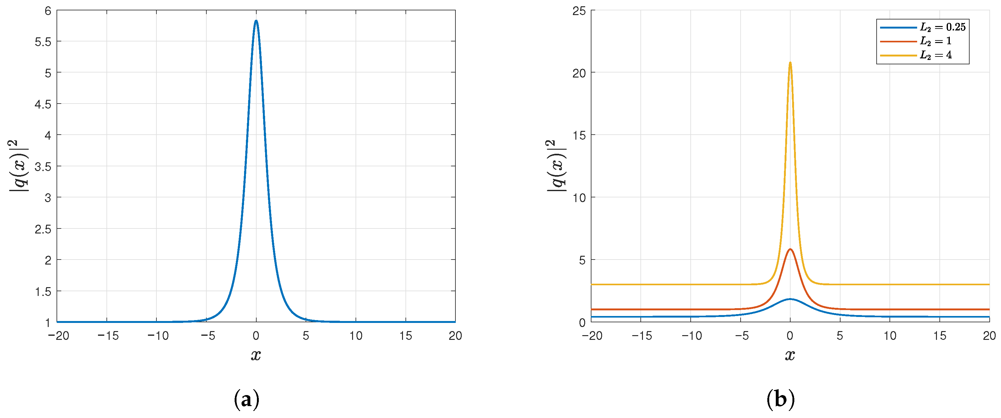
Case 1 of the enhanced direct algebraic method yields the bell-shaped (bright) quiescent soliton solution (19), for $L_2>0$, $L_4<0$ and ${\Delta }_{3l}>0$ under the algebraic constraints (Equation (18)). This family represents a localized intensity enhancement on top of a non-zero pedestal. The intensity profile $|q^{\left(l\right)}{(x,t)|}^2$ exhibits a single dominant peak with exponentially decaying tails, as illustrated in Figure 1a of the original manuscript, confirming its quiescent, non-propagating character.

The parameter $L_2$ plays a dual role: it controls both the peak amplitude and the spatial localization of the soliton. As $L_2$ increases, the peak intensity grows while the soliton width shrinks, leading to a more tightly localized structure, as shown in Figure 1b. Physically, this corresponds to tuning the balance between nonlinear CD and Kerr nonlinearity: higher effective $L_2$ represents stronger net focusing, which compresses the pulse spatially but increases the peak power. In the DWDM context, such bell-shaped quiescent solitons describe stationary energy concentrations in a given channel that can potentially seed instabilities or induce cross-talk via XPM, even though their centers do not drift.

5.2. Kink-Shaped and Singular Quiescent Solitons

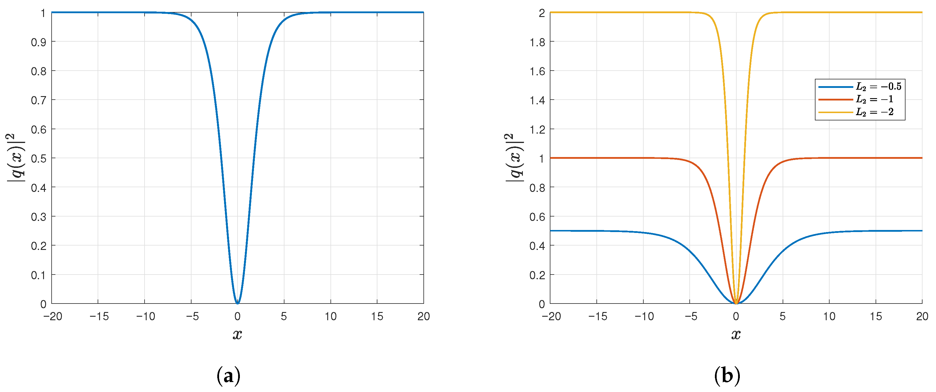
In Case 2, the enhanced direct algebraic method produces kink-shaped quiescent solitons of the form (23) again under suitable sign conditions on $L_2$, $L_4$ and ${\Delta }_{3l}$ and the constraints (22). The corresponding intensity profile $|q^{\left(l\right)}{(x,t)|}^2$ is a smooth transition between two distinct plateau levels, cf. Figure 2a. The solution is strictly quiescent: the kink location is fixed, and the transition is purely spatial.

The parameter $L_2$ modulates the slope of the transition and the separation between the plateau levels, as evident in Figure 2b. Larger $|L_2|$ yields sharper transitions and more pronounced contrast between the asymptotic states. Such kink-shaped quiescent solitons may be interpreted as domain walls between two stationary continuous-wave (FW) backgrounds in the same channel. In a DWDM system, they can act as stationary phase or amplitude fronts, potentially influencing neighboring channels through XPM without any longitudinal motion.

The same case also supports singular kink-like quiescent solutions with coth profiles. These correspond to unbounded intensities at a finite spatial point and thus represent limiting configurations that signal the onset of wave breaking or other catastrophic phenomena when the balance conditions are violated.

5.3. Straddled Quiescent Solitons

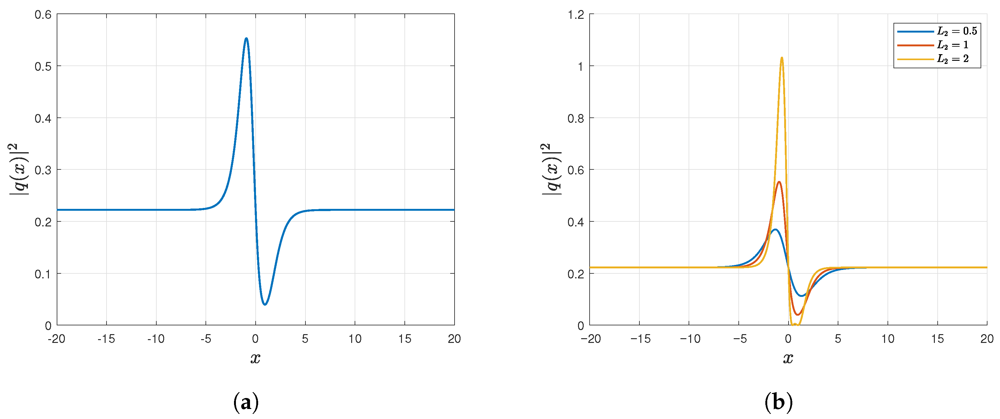
Case 5 leads to the straddled quiescent soliton solutions, characterized by more intricate hyperbolic combinations such as Equation (42) for $L_2>0$, $L_4>0$, ${\Delta }_{3l}<0$ and under the constraints of Equation (41). The intensity profiles in Figure 3a demonstrate a characteristic peak-dip structure: the soliton “straddles” the background, producing a localized region where the intensity first overshoots and then undershoots the asymptotic level (or vice versa).

Variations im $L_2$ significantly reshape the asymmetry between the peak and dip as well as their separation, as displayed in Figure 3b. From a physical point of view, these straddled quiescent solitons describe stationary localized defects with both enhancing and depleting lobes, making them particularly relevant in modeling trapped radiation or bound states of multiple localized modes within a single DWDM channel.

It is instructive to place these results in the context of earlier work. Previous analyses of the Schrödinger–Hirota equation and related higher-order NLSE models have mostly concentrated on traveling bright or dark solitons in single-channel fibers with linear chromatic dispersion, or on embedded/quiescent structures without DWDM coupling or nonlinear CD; see, for instance, Refs. [1,2,16,17,18,20,21,22,23,24]. In those settings only a limited set of localized profiles (typically pure bright, dark, or kink-type pulses) was obtained, and the parameter constraints were expressed in terms of a reduced subset of physical coefficients. The present study goes beyond these contributions by providing a systematic classification of stationary quiescent solitons for a DWDM Schrödinger–Hirota model with nonlinear CD, Kerr self–phase modulation, cross–phase modulation, and third–order dispersion. In particular, we obtain in closed form not only bell-shaped, dark, singular, and kink-shaped quiescent solitons, but also straddled and composite bright–dark configurations, together with their elliptic progenitors, all accompanied by explicit algebraic constraints that link the existence of each family to the underlying IMD, CD, SPM, XPM, and nonlinear dispersion coefficients. As far as we are aware, such a detailed parameter space description and taxonomy of quiescent dispersive solitons has not been reported before for DWDM systems with nonlinear chromatic dispersion.

These comparisons show that the present solutions do not merely replicate known solitary waves in a different notation, but instead reveal qualitatively new stationary patterns and parameter regimes that are directly relevant for the design and safe operation of dispersion-flattened DWDM fiber links.

5.4. Periodic Quiescent Solitons: Jacobi and Weierstrass Elliptic Families

Beyond isolated localized structures, the method also uncovers families of quiescent periodic solutions in terms of Jacobi elliptic functions (Case 3) and Weierstrass elliptic functions (Case 4). The former produce doubly periodic quiescent soliton lattices of cn-, dn-, and sn-type, as in Equations (27), (30) and (33), while the latter yield Weierstrass elliptic profiles of the form of Equations (37) and (38) with invariants $g_2$ and $g_3$ determined by the relations in Equation (39). These solutions describe stationary periodic wave trains where the amplitude is modulated in space but remains temporally quiescent.

Using classical relations between Weierstrass and Jacobi elliptic functions, the Weierstrass solutions can be re-expressed explicitly in terms of $\mathrm{cn}$, $\mathrm{sn}$, $\mathrm{dn}$ and $\mathrm{ns}$ functions, leading to a rich family of quiescent cnoidal and dnoidal waves (Equations (45)–(50)). In the limit $m\to 1$ (where m is the elliptic modulus), these periodic waves smoothly reduce to isolated solitons with hyperbolic profiles: the cn- and ns-based solutions degenerate to $\mathrm{sech}$ and coth, respectively, giving rise to so-called combo bright–dark quiescent solitons (Equations (47), (48), (51) and (52)).

From a physical standpoint, the elliptic families represent stationary pattern-forming states in the dispersion-flattened fiber. They may model quiescent soliton crystals or bound states, where multiple localized peaks are arranged periodically in space while remaining stationary in time. The ability to tune the elliptic modulus m provides a continuous transition from extended periodic waves to isolated quiescent solitons, offering a unified description of different regimes within the same DWDM platform.

5.5. Implications for DWDM Systems with Nonlinear Chromatic Dispersion

The broad spectrum of quiescent solutions—bell-shaped, kink-shaped, straddled, periodic and combo bright–dark—is a direct consequence of the nonlinear chromatic dispersion, higher-order dispersion and Kerr-type nonlinearities embedded in the SHE model. The analysis clearly indicates that the presence of nonlinear CD, encoded through the coefficient $b_l$ and the exponent R, substantially enriches the space of stationary states while also imposing delicate parameter constraints for their existence.

Because the solutions are quiescent, their centers do not drift along the fiber; instead, they form stationary spatial patterns. For DWDM systems this has a twofold implication. On one hand, such stationary structures can serve as robust traps or reservoirs of optical energy, potentially useful for buffering or for designing static nonlinear elements within the fiber. On the other hand, the same structures can be detrimental: a localized quiescent enhancement in one channel can induce persistent XPM on neighboring channels, and stationary domain walls or straddled patterns can seed modulation instabilities or polarization switching.

The concluding message of the analysis is therefore consistent: while nonlinear CD in dispersion-flattened fibers permits a rich zoo of dispersive quiescent solitons, it must be carefully controlled in practical DWDM deployments. Operating regimes that inadvertently push the system into the parameter ranges supporting strong quiescent structures may experience unexpected stationary distortions or cross-talk, with potentially severe performance penalties in long-haul DWDM links, including persistent inter-channel cross-talk and waveform distortion that translate into Q-factor degradation and BER penalties if not mitigated by dispersion/nonlinearity management.

6. Conclusions

The analysis presented in this work follows a coherent trajectory from the physical modeling of dispersion-flattened DWDM fibers, through the derivation of reduced profile equations, to the explicit construction and physical interpretation of quiescent solitons. By embedding each step within the existing body of work on higher-order Schrödinger-type equations and quiescent/embedded soliton dynamics, we aim to provide a logically connected and well-referenced framework for understanding stationary localized structures in Schrödinger–Hirota systems.

This paper recovered dispersive quiescent optical solitons whose basic model is SHE having nonlinear chromatic dispersion along with the Kerr law of the SPM structure. The enhanced direct algebraic method has made this retrieval possible through the intermediary functions, namely Jacobi’s elliptic functions as well as Weierstrass’ elliptic functions. The results of the paper portrays a telltale message to the optoelectronics community. The CD should not be rendered to be nonlinear at any stage during the pulse propagation for intercontinental distances. Thus significant signal-quality degradation may occur (e.g., distortion, ISI and cross-talk), reducing transmission reach and increasing BER unless appropriate dispersion and nonlinear-impairment mitigation are employed. Therefore, it is imperative for the telecommunication engineers to exercise extreme caution to make sure that the CD is never nonlinear during the course of the pulse transmission through such dispersion-flattened fibers.

Compared with the available literature on Schrödinger–Hirota and higher-order NLSE models, the present work makes several contributions that, taken together, are, in our opinion, substantial. First, we formulate and analyze a DWDM Schrödinger–Hirota model with nonlinear chromatic dispersion specifically tailored to dispersion-flattened fibers, and we rigorously reduce it to a quartic stationary profile equation whose coefficients retain a clear physical meaning. Second, by adapting and extending the enhanced direct algebraic method, we derive a broad family of exact quiescent dispersive solitons (bright, dark, singular, kink-shaped, straddled, elliptic, and composite bright–dark) together with explicit existence constraints that delineate narrow regions in the multidimensional parameter space of the DWDM system. Third, we show how the Weierstrass elliptic solutions can be systematically transformed into Jacobi elliptic and hyperbolic forms, thereby uncovering additional cnoidal and combo structures that do not appear in previously studied settings. Finally, we interpret these findings in terms of realistic fiber parameters and emphasize their implications for the robustness and potential vulnerability of long-haul DWDM links. These features, in combination, provide a new and coherent picture of stationary localized structures in dispersion-flattened fibers and, we believe, justify the relevance of the present study for the readership of this journal.

In addition to recovering a broad catalog of quiescent soliton and elliptic-type solutions, this work has clarified how nonlinear chromatic dispersion, Kerr self-phase modulation, cross-phase modulation, and higher-order dispersive effects jointly shape the parameter regimes in which such static structures can exist in dispersion-flattened DWDM systems. By formulating and analyzing the generalized Schrödinger–Hirota model, and by implementing the enhanced direct algebraic method in a systematic way, the paper provides a unified analytical framework that encompasses bright, dark, singular, Jacobi elliptic, Weierstrass elliptic, combo, and straddled quiescent optical solitons, together with explicit constraint conditions that are directly interpretable in terms of physical system parameters.

Several avenues for future research naturally emerge from the present study. A first step is to carry out a detailed numerical stability and perturbation analysis of the obtained quiescent soliton families under realistic effects such as higher-order dispersion, Raman scattering, self-steepening, gain/loss, and stochastic noise, in order to assess their robustness over long-haul transmission. Further extensions of the model to incorporate nonlocal or saturable nonlinearities, birefringence, polarization dynamics, and coupled-core geometries may reveal new classes of vector and multi-component quiescent solitons. It is also of interest to investigate higher-dimensional and $\mathcal{PT}$-symmetric generalizations of the Schrödinger–Hirota equation, building connections with recently reported multidimensional and strange wave structures. Finally, quantitative comparison with experimental or high-fidelity numerical data from dispersion-flattened DWDM platforms would help validate the analytical profiles reported here and guide the design of practical soliton-based optical communication schemes that either exploit or deliberately avoid such quiescent structures.