Abstract
Background: Realistic simulation of ECG signals is essential for validating signal-processing algorithms and training artificial intelligence models in cardiology. Many existing approaches model either waveform morphology or heart rate variability (HRV), but few achieve both with high accuracy. This study proposes a hybrid method that combines morphological accuracy with physiological variability. Methods: We developed a mathematical model that integrates Gaussian mesa functions (GMF) for waveform generation and a chaotic Rössler attractor to simulate RR-interval variability. The GMF approach allows fine control over the amplitude, width, and slope of each ECG component (P, Q, R, S, T), while the Rössler system introduces dynamic modulation through the use of seven parameters. Spectral and statistical analyses were applied, including power spectral density (PSD) computed via the Lomb–Scargle, STFT, CWT, and histogram analyses. Results: The synthesized signals demonstrated physiological realism in both the time and frequency domains. The LF/HF ratio was 1.5–2.0 when simulating a normal rhythm and outside these limits in a simulated stress rhythm, consistent with typical HRV patterns. PSD analysis captured clear VLF (0.003–0.04 Hz), LF (0.04–0.15 Hz), and HF (0.15–0.4 Hz) bands. Histogram distributions showed amplitude ranges consistent with real ECGs. Conclusions: The hybrid GMF–Rössler approach enables large-scale ECG synthesis with controllable morphology and realistic HRV. It is computationally efficient and suitable for artificial intelligence training, diagnostic testing, and digital twin modeling in cardiovascular applications.
1. Introduction
Electrocardiography (ECG) is a fundamental method for monitoring and diagnosing cardiac activity, providing critical information about the electrical activity of the heart. Mathematical modeling of realistic ECG signals enables the testing and evaluation of new analysis algorithms [1], the replacement of corrupted segments in real cardiac data, noise reduction, and baseline drift removal [2], as well as signal classification [3] and artificial intelligence training. One of the most commonly used approaches for ECG signal modeling is based on Gaussian functions [4], which allow precise reproduction of the morphology of the P-wave, QRS complex, and T wave through parameterized mathematical expressions. Although this morphological approach provides flexibility and accuracy in representing individual waves, it does not fully capture the natural variability and dynamic properties of heart rhythm.
To achieve a more realistic representation of heart rate dynamics, the present study integrates a chaotic component, based on the Rössler attractor [5], into the morphological ECG model. The Rössler attractor is known for its complex yet structured nonlinear dynamics, which can simulate the natural variations in RR intervals characteristic of normal cardiac function and certain pathological conditions. By combining Gaussian functions for wave morphology modeling with a chaotic model for heart rate control, a hybrid ECG synthesis method is developed, capable of reproducing both normal and arrhythmic conditions.
This study presents an algorithm for synthesizing ECG signals using a combined morphological and dynamic approach, aiming to achieve a more realistic representation of the intrinsic dynamics of this nonlinear, quasi-periodic signal. Particular attention is given to the impact of chaotic dynamics on heart rate variability (HRV) and the ability to generate different ECG waveform patterns by parameterization of the attractor.
Related Works on Methods for the Generation of ECG Data
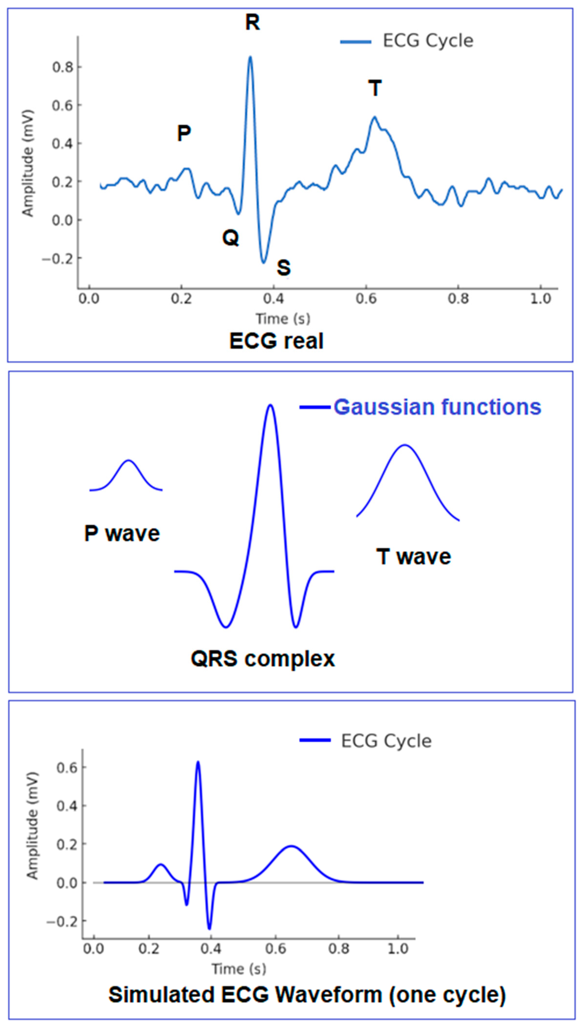
In mathematical modeling of ECG signals, three main approaches can be distinguished: morphological models, dynamic models, and physiological models. These models describe the standard shape of the ECG signal (Figure 1), including its characteristic P, QRS, and T waves, using a single equation, a superposition of functions, or a system of differential equations. In [6], a simplified computational model with low computational cost was proposed, modeling ECG signals using only two Gaussian functions and applying two different methods for optimizing the model parameters.
Figure 1.
ECG (modeled using standard Gaussian functions).
The authors of [7] applied a Gaussian model to represent the primary electrocardiographic waves. They utilized the local peaks and extrema of these key features to synthesize the ECG signal as a sum of six Gaussian functions. To improve morphological accuracy, ref. [8] introduced a method using eight Gaussian functions with optimized parameterization, ensuring a more precise depiction of the individual characteristics of the P, QRS, and T waves. A combined approach involving two Gaussian functions and sinusoidal components (via Fourier analysis) was used in [9] for enhanced ECG signal reconstruction. A method describing characteristic waves with Gaussian mesa functions (GMS) was proposed in [10], where the functions were combined using a generalized orthogonal forward regression algorithm, resulting in a model composed of six Gaussian mesa functions, each representing a specific segment of the ECG waveform. The authors also proposed the use of Bi-Gaussian Functions (BGFs). The basic concept of the morphological model is illustrated in Figure 2.
Figure 2.
Basic concept of the morphological model.
In addition to Gaussian functions, the ECG waveform can also be represented using Hermite interpolating polynomials [11,12] or as a sum of sinusoidal functions through Fourier and discrete cosine transforms (DCT) [13,14]. In [15], a general framework for morphological modeling of ECG signals was introduced, where the signal is represented as a sum of basis functions with scaling coefficients for width and amplitude. Both general and specific variants of the model were described, with three techniques explored: McSharry’s model, a sinusoidal model, and a spline-based model. The goal of this framework is to minimize the error between synthesized and actual ECG signals by optimizing both the basis functions and their expansion coefficients.
Dynamic models. A fundamental contribution to this field is the McSharry model [16], which employs three nonlinear differential equations to describe heart rhythm dynamics in a three-dimensional phase space. This model incorporates an attractor that regulates signal behavior based on three main components: the QRS complex, the P-wave, and the T wave. At its core, the model assumes harmonic motion around a toroidal attractor, where the position and shape of the waves are controlled by phase parameters related to time and heart rate. The model generates a standard sinus rhythm characteristic of a healthy individual. Additionally, two Gaussian functions are applied to introduce variability into the synthesized time series, affecting both its low-frequency and high-frequency spectra. This model is widely used for generating synthetic ECG signals that retain the physiological characteristics of real recordings, making it suitable for testing biomedical signal-processing algorithms. References [17,18,19,20] present modified versions of the McSharry model.
The Zeeman model for ECG is a nonlinear dynamic model [21,22] based on catastrophe theory, which describes the cardiac time series as a result of sudden transitions between stable states. It utilizes bifurcations and abrupt changes within the system to explain the rapid rise and fall in voltage during cardiac depolarization. This model represents the electrical activity of the heart through nonlinear differential equations that describe transitions between different attractors. It is particularly useful for modeling sudden transitions in ECG signals and can be extended for analyzing arrhythmias and pathological conditions.
Physiological models are based on reproducing the activity of cardiac tissue at the cellular level [23], using mathematical descriptions such as differential equations, nonlinear oscillators [24], and other related methods.
In recent years, deep generative modeling has become a major focus in synthetic ECG research, introducing capabilities that go beyond classical morphological and dynamic models. Recent studies, such as the scoping review [23], have reviewed the literature on ECG synthesis and highlighted the growing influence of deep learning-based methods, including generative adversarial networks (GANs), variational autoencoders (VAEs), and diffusion models. GAN-based ECG generators have been used to synthesize multichannel rhythms and arrhythmias while improving data augmentation pipelines; examples include TimeGAN, conditional ECG-GAN architectures, and the clinically oriented CLEP-GAN [25], which reconstructs ECGs from PPG signals using adversarial domain translation. Diffusion-based approaches have also emerged, offering improved robustness and higher-quality waveform generation. For example, ref. [26] uses a diffusion model + state-space transformer for 12-lead ECG. Ref. [27] presents text-to-ECG synthesis for 12-lead. Ref. [28] demonstrates the generation of multi-bit ECG sequences with differentiation and preserved inter-bit dependencies. The study by diffusion-based conditional ECG generation with structured state-space models (SSSD-ECG) [29] introduces a diffusion-model framework conditioned on clinical state variables to generate physiologically realistic ECG sequences.
Within the deep learning family, diffusion-based generators and state-space-aware architectures have emerged as the most promising class for 1D biosignal synthesis in 2023–2024, providing probabilistic sampling, improved mode coverage, and flexible conditional generation for heart rate imputation and prediction. Representative examples include DiffECG [30] and BeatDiff [31], as well as state-space transformation models such as ECG-Mamba [32], all of which report very good waveform accuracy compared to earlier GAN- and autoencoder-based generators. GAN approaches remain widely used for ECG augmentation and classifier training [33], and transformer-based morphology synthesis continues to evolve [34].
There were no pure attractor–chaos models published in the literature in 2023–2025, which indicates that hybrid methods combining deep learning with nonlinear attractors are still lacking. Only [35] proposes a modified version of McSharry’s model. This study presents a new synthetic ECG signal generator that uses chaotic dynamics instead of standard pseudorandom methods to more realistically capture the variability between individual heartbeats. A fourth-order memristor circuit generates the chaos, allowing precise control over the characteristics of the ECG signal peaks, both in software and hardware implementation.
In addition to stand-alone signal synthesis, the proposed GMF–Rössler generator can be natively embedded in emerging cardiac digital twin (DT) frameworks. Recent developments, such as the Heart DT platform [36], combine IoT ECG sensors, microservices-based processing, and deep learning classifiers to build a cloud architecture for real-time monitoring and prevention of cardiac pathologies.
In parallel, cardiac digital twins and “cardio twin” architectures have been proposed as patient-specific virtual copies of the heart that use ECG-based AI models to support cardiac treatment and clinical decision-making [37,38,39,40,41,42].
Within these ecosystems, the hybrid GMF–Rössler model proposed in this paper can serve as a synthetic data engine that supplements clinical ECG streams with controllable virtual signals for pre-training and stress-testing of CNN/LSTM classifiers of the DT AI layer. It can also act as a scenario simulator in which HRV parameters, attractor settings, and noise levels are systematically varied to emulate different physiological states (rest, fatigue, and stress) and sensor artifacts before deploying it on real patients. The model can be integrated at the end of the DT stack, near wearable ECG devices, to generate personalized “what-if” trajectories that are continuously recalibrated against the patient’s observed HRV statistics, thereby supporting promising applications of digital twins in arrhythmia risk stratification, remote monitoring, and adaptive therapy optimization.
2. Materials and Methods
Hybrid model based on Gaussian functions and the Rössler attractor.
Simulating an electrocardiogram using Gaussian functions is a morphological approach that employs mathematical representations to replicate the primary waves in an ECG signal—P-wave, QRS complex, and T wave. This method is based on the superposition of Gaussian curves, where each wave is modeled as a separate function with specific amplitude, width, and temporal location. The advantage of this approach lies in its flexibility in adjusting waveform morphology, allowing for the realistic reproduction of both physiological and pathological variations. While dynamic and chaotic models focus on temporal dependencies and autonomic modulation in heart rhythm, the morphological model emphasizes the shape and structure of cardiac potentials, making it particularly useful for analyzing and simulating various cardiac conditions.
In modeling with Gaussian Distribution Functions (GDF), each Gaussian function is described by the following [1]:
where
- A—Amplitude, determining the peak height of the wave;
- μ—Central position in time (defines when the wave appears in the cycle);
- σ—Standard deviation (defines the width and smoothness of the wave);
- t—Time variable.
Physiologically, the ECG signal recorded at the body surface results from the spatial summation of potentials generated by multiple active cardiac regions, including atrial and ventricular depolarization and repolarization.
According to the bidomain model of cardiac electrophysiology [43,44,45], these distributed current sources contribute linearly to the observed surface potential under the quasi-static approximation, where magnetic effects are negligible. Therefore, the body-surface ECG can be mathematically represented as the linear superposition of wave components corresponding to the major cardiac events:
The index i corresponds to different waves (P, Q, R, S, T):
- P-wave—Models the initial depolarization of the atria. It is smooth and rounded and can typically be well-described by a single Gaussian function.
- QRS complex—This is a fast and sharp transition, requiring three separate Gaussian functions to model its shape:
- Q-wave—A short, small negative deflection;
- R-wave—A tall and sharp peak, and the most prominent part of the signal;
- S-wave—A brief negative drop following the R-wave;
- T wave—It can be well-described with two Gaussian functions due to its wider and more rounded shape, which requires greater flexibility for accurate modeling.
This additive formulation provides a physiologically consistent and computationally efficient approximation of the combined electrical activity of the heart. Similar morphological models [1,15,16] using Gaussian basis functions have been validated in the literature and shown to accurately reproduce ECG waveforms for both normal and pathological conditions.
The use of GDF has gained widespread adoption in ECG modeling; however, it does not account for the fact that the waves of this dynamic signal are not perfectly symmetrical. To generate a broader range of realistic waveforms observed in actual ECG signals, the Gaussian mesa function (GMF) model [10] is a suitable alternative. In this model, two Gaussian functions are used for each wave to better capture the asymmetry at the beginning and end of the waveform. GMF is an extended version of the Gaussian function with a flattened peak and more flexible parameters, enabling modeling of realistic physiological signals such as ECG. The GMF is defined as a partial combination of two half-Gaussian segments and a constant plateau:
where
- μ—Temporal location, defining the position of the wave along the time axis;
- —Width of the first half-Gaussian function, defining the spread of the initial part of the wave;
- —Width of the second half-Gaussian function, defining the spread of the latter part of the wave;
- —Plateau duration, determining the length of the horizontal segment between the two half-Gaussian functions;
- A—Amplitude, defining the wave height.
Advantages of the GMF Model:
- -
- The QRS complex in ECG exhibits a sharp peak but is not perfectly symmetrical; a single Gaussian function would result in an idealized, less realistic shape;
- -
- GMF allows for a more realistic modeling of the QRS complex, where two Gaussian components with different parameters can better represent the steep ascending phase and the less steep descending phase of the signal;
- -
- This method reduces reconstruction errors when generating synthetic ECG signals in real-time.
Each ECG wave is modeled using a fixed GMF parameter set (, ), where the subscript i ∈ {P,Q,R,S,T} identifies the corresponding wave. Each wave has its own independent parameter group, allowing the complete ECG cycle to be represented as a sum of five GMF components. In this formulation, the P-wave is modeled with a single mesa function with a relatively small amplitude its temporal position is determined by the parameter , while its morphology is controlled by three shape parameters: the rising slope, the falling slope , and the plateau width .
Together, these parameters define the smooth, low-amplitude shape of the P-wave. The QRS complex is described using three GMF components—Q, R, and S—each with distinct temporal offsets ,, and asymmetric widths that capture the steep rise and fall of the depolarization phase. The T wave uses one GMF component with a longer plateau to model its broader morphology. This explicit allocation ensures that the five cardiac events are controlled independently (Table 1), while the final ECG signal is obtained as the superposition of all GMF waveforms.
Table 1.
Allocation of GMF parameters for each ECG wave.
By combining Gaussian functions for morphological representation with chaotic attractors for dynamic modeling, this approach ensures that the synthetic ECG signal retains all key physiological characteristics of a real cardiac cycle.
The use of a chaotic model based on attractors or stochastic variations allows for the introduction of the natural variability of RR intervals, which is characteristic of a healthy heart rhythm and certain arrhythmias. The Rössler attractor [46] is a chaotic dynamic system used for modeling biological and physiological processes and may be suitable for embedding variations in heart rhythm. It can replicate the natural nonlinearity and dynamics of RR intervals, which are characteristic of normal cardiac activity.
The Rössler attractor system is well-suited for describing chaotic dynamics with fractal properties [47]:
where this equation denotes the state vector of the Rössler system. The dynamics are governed by the following system of nonlinear differential equations:
where x, y, z are the state variables, and a, b, c are the system controlling the degree of chaotic behavior.
2.1. Numerical Integration: Runge–Kutta Methods
To obtain a numerically stable and accurate trajectory of the chaotic attractor, the Rössler system was solved using explicit Runge–Kutta methods of order p. The general s-stage Runge–Kutta scheme for a system of ordinary differential equations is defined as follows:
The choice of the classical fourth-order scheme (RK4) provides a local truncation error of O() and a global error of O(). For long-term simulations (e.g., 12-h ECG synthesis), higher-order variants such as RK6 or adaptive schemes (e.g., DOP853) may be employed to ensure numerical stability and minimize cumulative error.
The Rössler subsystem was integrated using a fixed-step RK4 method with Δt = 0.001 s. Convergence was verified by repeating the simulations with Δt = 0.0005 s, resulting in negligible differences in HRV metrics (<1%).
To ensure that the numerical integration is both convergent and stable for long simulated ECG sequences, we performed a more detailed grid-refinement and stability analysis using fixed-step Runge–Kutta schemes.
For numerical convergence, simulations were repeated with a refined step Δt = 0.0005 s, and the resulting RR sequences and ECG waveforms were compared. The relative differences in HRV metrics (mean RR, SDNN, RMSSD, and LF/HF) remained below 1%, and the maximum pointwise deviation in the synthesized ECG amplitude did not exceed 0.03 mV. These results confirm first-order convergence in RR timing (due to discrete beat detection) and fourth-order convergence in the continuous attractor trajectory (due to RK4).
For stability verification, we simulated extended sequences of up to 2 h using the same fixed step. No divergence, oscillatory growth, or accumulation of numerical drift was observed. The attractor trajectory remained confined to its bounded region, and all RR intervals remained strictly positive and within their physiological limits.
Finally, repeated simulations with different random seeds for the additive physiological noise term produced consistent HRV statistics, demonstrating robustness to stochastic perturbations.
2.2. Attractor–Timing Coupling: A Dimensionless Derivation
The goal of this subsection is to establish a physiologically consistent and dimensionally correct mechanism for coupling the chaotic Rössler attractor with the temporal HRV. In the proposed framework, the attractor only modulates the RR intervals (i.e., inter-beat timing) and does not multiply the ECG amplitude.
The Rössler system (3) is numerically integrated using a time step Δt, producing an internal trajectory in an abstract time domain without physical units.
To align the dominant chaotic timescale with physiology (~1 Hz), a dimensionless time-scaling factor is introduced and defined:
where is chosen so that the dominant oscillation in approximates 1 Hz, corresponding to a heart rate of about 60 bpm.
The attractor state is normalized to obtain a unit-free process:
where and are the mean and standard deviation of computed over the simulation horizon. This normalization guarantees that is dimensionless and suitable for timing modulation.
To incorporate the chaotic fluctuations into HRV, the sequence of RR intervals is generated using a dimensionally consistent exponential map:
where denotes the mean RR interval (ms), and α is a small dimensionless coefficient controlling the strength of HRV ().
Although the Rössler subsystem introduces deterministic chaotic variability, physiological HRV also contains an inherently stochastic component. To incorporate this natural randomness, we extend the RR-interval model by adding a zero-mean stochastic term
where is an additive Gaussian noise term with variance , controlling the strength of physiological randomness.
This formulation guarantees that all values remain positive and physiologically valid.
The time of the next heartbeat is computed recursively as follows:
In this way, the chaotic attractor influences only the timing variability of the ECG sequence, rather than its amplitude.
Once the temporal modulation is determined, the ECG waveform for each beat is synthesized as a sum of GMFs representing the P, Q, R, S, and T waves:
where , define the amplitude, temporal location, and asymmetry of each component.
The representation of this complete hybrid dynamical model that combines the chaotic Rössler subsystem, the discrete RR-interval dynamics, and the GMF-based ECG morphology is as follows:
where is the dimensionless, normalized attractor state, , are the Gaussian mesa function parameters for the ECG waves , and denotes the final synthesized ECG signal.
Stepwise Description of algorithm of ECG Synthesis Using Gaussian Mesa Functions and the Rössler Attractor.
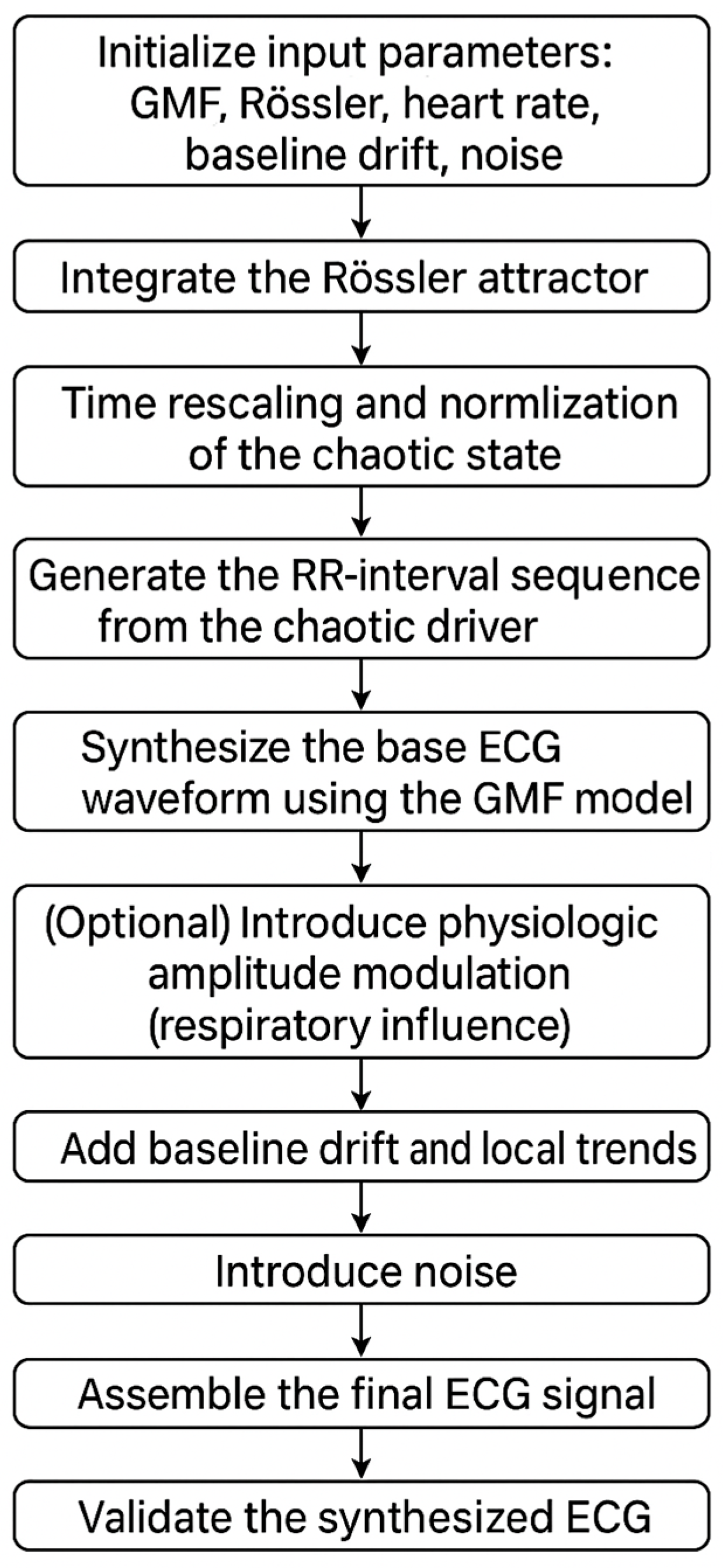
The algorithm of the proposed method is presented in Figure 3.
Figure 3.
Flowchart of the proposed hybrid ECG synthesis algorithm combining Gaussian mesa functions and the Rössler attractor.
- 1.
- Initialize input parameters:Morphological (GMF) parameters for each wave :where is amplitude, , is temporal offset, control asymmetric rise/decay, and is the plateau duration.Rössler attractor parameters:where a, b, c are system parameters,are initial conditions, is the time-scaling factor, and α controls the strength of HRV modulation.Heart rate and sampling parameters:mean RR interval umber of heartbeats N, and sampling frequency .Baseline drift and noise parameters:, for drift,, for high- and low-frequency components, and the variance of additive Gaussian noise.(Optional) Respiratory amplitude modulation parameters: .
- 2.
- Integrate the Rössler attractor.Solve the Rössler system (4) numerically using a Runge–Kutta scheme with time step Δt generating the trajectory over the desired simulation horizon.
- 3.
- Time rescaling and normalization of the chaotic state—with Equations (8) and (9).
- 4.
- Generate the RR-interval sequence from the chaotic driver—with Equations (10) and (11).
- 5.
- Synthesize the base ECG waveform using the GMF model—with Equation (13).
- 6.
- (Optional) Introduce physiologic amplitude modulation (respiratory influence)To emulate slow, non-chaotic amplitude variability due to respiration, modulate the GMF amplitudes by a low-frequency sinusoid:.The time-dependent amplitudes replace the constant it Step 5 (Equation (12)).
- 7.
- Add Baseline Drift and Local Trends:
- -
- Introduce slow baseline drift using the follows:where is random phase, is a Gaussian step, and controls the strength of the unstable drift.
- -
- Choose ∈ [0.01, 0.3] mV and ∈ [0.01, 0.1] Hz.
- -
- Add a linear local trend if simulating long-term ECG signals.
- 8.
- Introduce Noise:Generate and add different types of noise:High-frequency noise (electrical interference, EMG artifacts) is as follows:where is white Gaussian noise passed through an HPF (high-pass filter) (cutoff: 20–30 Hz) to mimic broadband EMG fluctuations.Low-frequency noise (respiratory influences, baseline wander) is as follows:where is white Gaussian noise passed through an LPF (low-pass filter) to reflect slow, irregular respiratory oscillations.Additive stochastic noise ε(t), typically zero-mean Gaussian.The total noise term is as follows:
- 9.
- Assemble the Final ECG Signal.Combine all components:Normalize and scale the signal to fit standard ECG ranges (−1.5 to 2.5 mV).
- 10.
- Validate the Synthesized ECGHRV analysis: Compute time-domain and frequency-domain metrics.Spectral analysis: Apply STFT and CWT to confirm realistic frequency components.
- 11.
- Save and Export the Synthetic ECG for Further Analysis.
The model allows fine control over waveform shape, temporal variability, noise, and baseline drift, making it suitable for biomedical research, AI model training, and validation of ECG processing algorithms.
Table 2 presents the configuration parameters used to generate synthetic ECG signals for rest, fatigue, and stress, including the input values for RR intervals, GMF morphology, and Rössler attractor parameters. The Rössler attractor parameters are chosen to maintain stable chaos, but with varying degrees of instability, and the method was initially investigated with a = 0.2, b = 0.2, and c = 5.7 (which are standard Rössler attractor values). The GMF parameters (heights and widths) are calibrated to typical ECG values, allowing for asymmetry between the left and right slopes. The combination of RR dynamics and morphological modeling aims to achieve high physiological reliability of the synthetic signal. To simulate fatigue and stress states, the GMF parameters were adapted by lowering the wave amplitudes, changing the widths, and adding different types of noise with different amplitudes to mimic real-world artifacts and variations.
Table 2.
Configuration parameters for simulating different physiological states.
- Parameter Justification and Sensitivity Considerations
The parameter triplet (a,b,c) in the Rössler system was selected according to established dynamical properties of the attractor and their correspondence with physiological heart rate modulation. Parameter a regulates the oscillatory rotation rate and thus modulates low-frequency variability; parameter b has a weak effect on amplitude contraction and is kept constant; parameter c controls chaotic intensity and governs irregularity in the RR time series. A local sensitivity exploration (±10–20% perturbations around the baseline values) confirmed that the synthesized RR series remained within physiological HRV ranges (SDNN ≈ 55–75 ms, RMSSD ≈ 45–65 ms, and LF/HF ≈ 1.2–1.8). Thus, the selected parameter sets provide physiologically realistic modulation without requiring extreme tuning.
- Boundedness and Stability Analysis
Let us show that the hybrid model remains bounded and, with appropriate parameters, satisfies the following:
- 1.
- Dimensionless chaotic input (timing only).The Rössler state is normalized (Equation (9)) and used solely to modulate RR intervals (see Equations (8)–(14)), and hence it does not scale the ECG amplitude. This removes any direct route for unbounded growth via chaos.
- 2.
- Positive and bounded RR intervals.RR intervals are generated by the exponential map extended with a stochastic component (Equation (11)), where is zero main physiological noise.This is due to the following: for all is constrained such that ; we have ensuring strictly increasing beat times in Equation (12). Thus, the temporal dynamics of the ECG remain well-defined.Additionally, the model uses ∣α∣ ≪ and clipping (e.g., ), which yields ∈ [, ] with > 0, so beat times are well-defined, and the number of overlapping beats around any t is finite.This guarantees both positivity and boundedness of the inter-beat timing.
- 3.
- Bounded morphology.
Each GMF component satisfies for all t. Let
By construction, the following:
Thus, the morphology of each beat is strictly bounded.
- 4.
- Controlled overlap of successive beats.Let W be the effective support of a beat (plateau plus 5 max ()). Choosing } (rest and fatigue) implies no inter-beat overlap ( = 1). For stress, where may approach W, we upper-bound the local overlap by (empirically valid for our parameter sets). Thus, at any time, we have the following:
- 5.
- Bounded drift and noise.
We generate baseline drift and additive noise with fixed bounds:
- 6.
- Global amplitude bound.By the triangle inequality, we have the following:Hence, imposing the following:guarantees [−2, 2] mV.
In our experiments, we use, for example, , with = 1 (rest, fatigue) and (stress), which satisfies (26).
Statistical analysis
All statistical tests were two-sided with a significance level of α = 0.05. Analyses were performed separately for the real and simulated HRV metrics (MeanRR, SDNN, RMSSD, LF/HF, etc.) across the three physiological states (rest, fatigue, and stress). All computations were implemented in Python (v3.11) using the scipy.stats and statsmodels.api libraries.
Normality test (Shapiro–Wilk). For each HRV variable, the null hypothesis is as follows:
: The data drawn from a normal distribution was tested using the Shapiro–Wilk statistic:
where are the ordered sample values, is the sample mean, and are tabulated coefficients depending on n. Small W with indicates a rejection of normality.
Paired-sample t-test. For each HRV parameter, real and simulated values were compared within the same subject using a paired two-sided t-test. The null hypothesis is as follows:
where
are the paired differences, and they were evaluated using the test statistic:
where and denote the mean and standard deviation of differences, respectively.Cohen’s was reported as an effect size.
H0: E[d] = 0,
Correlation analysis. The linear relationship between real and simulated HRV metrics was quantified using the Pearson correlation coefficient:
with the following null hypothesis:
:
Confidence intervals for r were obtained via Fisher’s z-transformation:
Results include the test statistic (W, t, r), corresponding p-values, 95% confidence intervals, and effect sizes (Cohen’s , correlation r).
All tests were two-sided, and results were considered significant at <0.05.
Participants.
Thirty-six Bulgarian wrestlers (male, 100%; age: 20.6 ± 2.3 years) voluntarily participated in the study. All participants were clinically healthy at the time of enrollment. The athletes represented club teams from central Bulgaria.
Three ECG recordings were performed for each participant: (1) in a resting state before training, (2) immediately after its completion, and (3) two hours later.
A total of 114 ECG recordings (38 athletes × 3 physiological states) were initially collected. Three recordings from 2 participants (2.63%) contained uncorrectable artifacts. Since the study design required a complete set of three recordings per participant, the two affected athletes were excluded entirely, resulting in the removal of 6 recordings (5.26%) for methodological reasons. The final dataset, therefore, consisted of 108 valid recordings (94.74%).
ECG signals were recorded with a Holter device (TLC9803) in the second lead, lasting 10 min. Data from the third to the tenth minute (8 min) were used for analysis to ensure signal stabilization and to avoid artifacts at the beginning of the recording.
The simulated ECG signals also included 36 recordings for each physiological state, with a duration of 8 min.
2.3. Spectral Analysis
- Short-Time Fourier Transform (STFT)
The continuous STFT of a signal x(t) with analysis window (⋅) is as follows:
In discrete time (sampling rate ), using window length L, hop size H, FFT size K, and frame index m, we compute the following:
The spectrogram is obtained as follows:
where
ensures power normalization. The frequency is given by the following:
Continuous Wavelet Transform (CWT)
For mother wavelet ψ the CWT is as follows:
with scale a ∈ R∖{0} and time shift b ∈ R. We use the complex Morlet wavelet
with central frequency ( = 1 in normalized units). The scale–frequency mapping is in continuous time; in discrete time with Δt = 1/ and the wavelet center frequency. The scalogram is as follows:
and when reported versus f, we write the following:
We indicate the cone of influence near the boundaries. The Morlet satisfies the wavelet admissibility condition (finite ).
- Power Spectral Density (PSD)
The continuous-time PSD is as follows:
with
In discrete time, we estimate PSD via Welch’s method: segment the signal into M overlapping windows of length K (overlap 0 < γ < 1), apply window w[n], and average periodograms:
To provide a more comprehensive and quantitative assessment of the similarity between real ECG signals x[n] and the simulated ECG signals , in addition to the correlation coefficient, the root mean square error (RMSE) and the Dynamic Time Warping (DTW) were calculated, which capture both amplitude and temporal (morphological) deviations between pairs of signals:
where N is the number of samples in each signal.
The DTW distance quantifies morphological and temporal dissimilarity by finding the optimal alignment path between the two signals:
where W denotes the warping path and d(⋅,⋅) is a local distance measure (typically the squared Euclidean distance).
3. Results
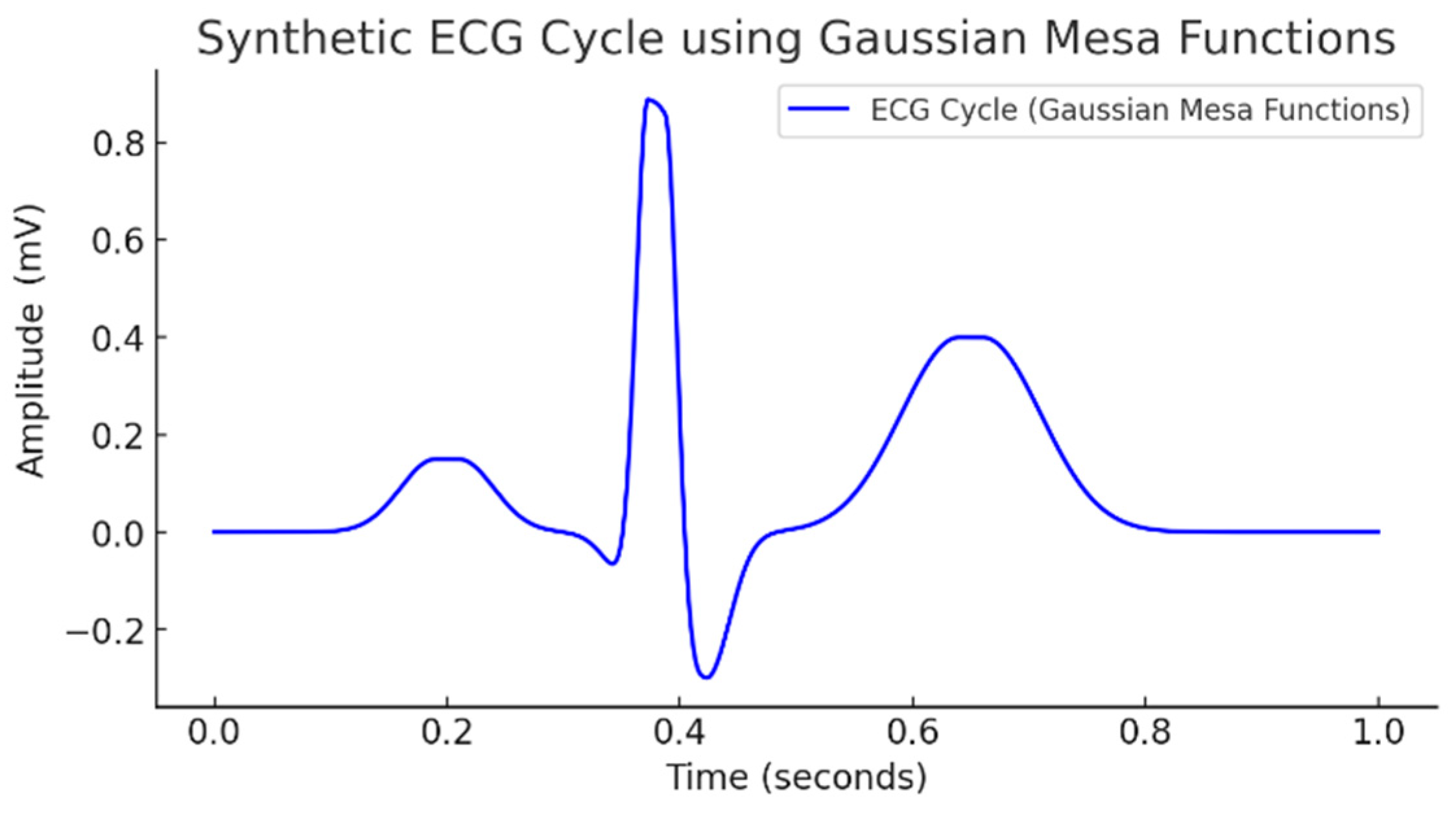
The basic ECG model in this study was implemented with a Gaussian mesa function (Figure 4), which allows for the adjustment of each of the slopes of each wave separately and the width of the wave plateau to be set.
Figure 4.
Synthetic ECG cycle using Gaussian mesa functions.
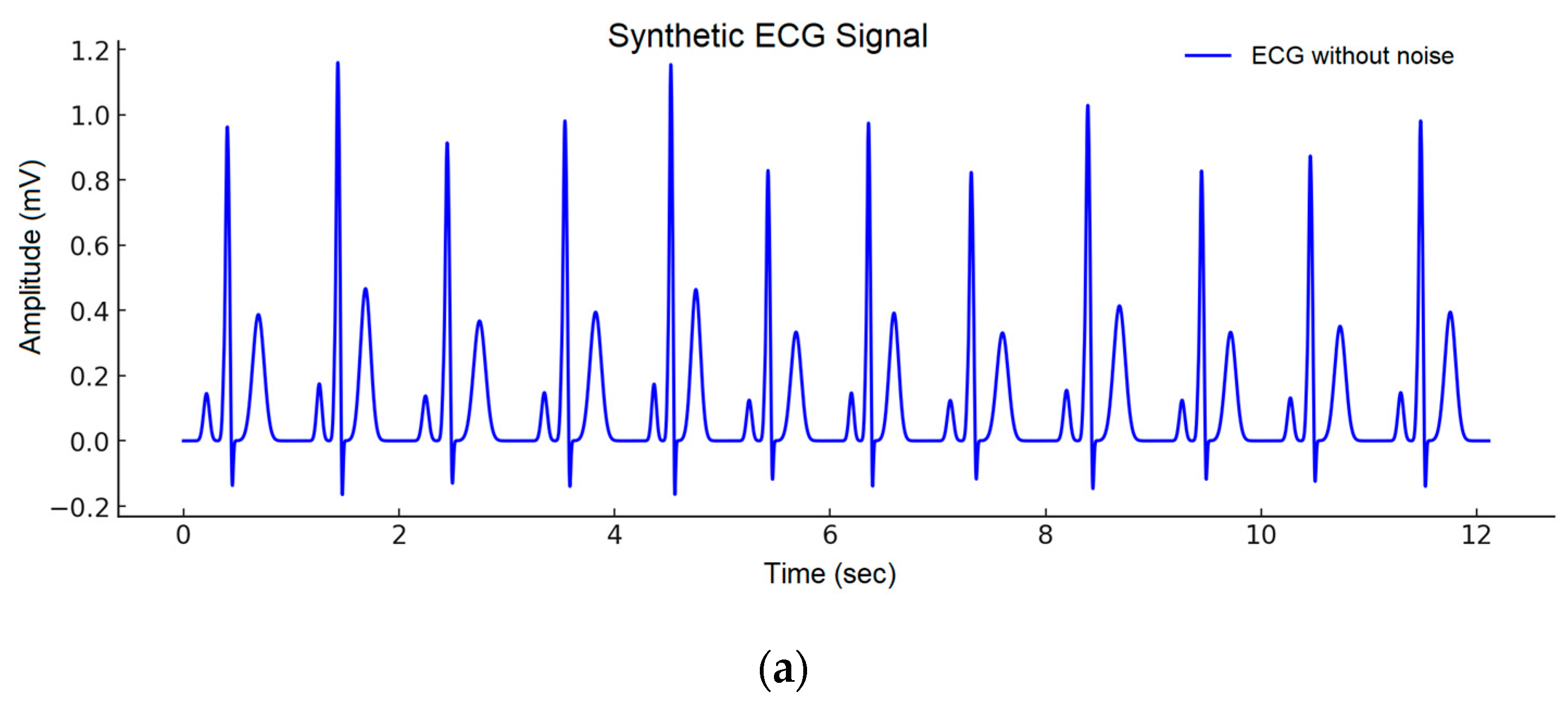
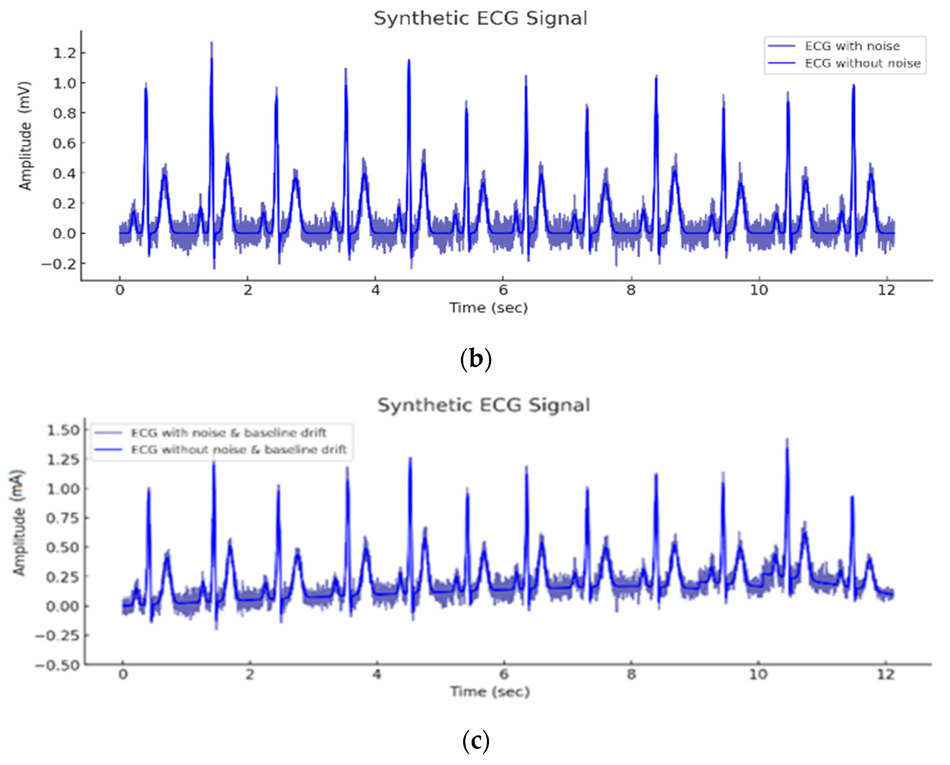
Figure 5a presents a synthesized ECG cycle generated using the Gaussian mesa function (GMF) model with parameters calibrated to mimic a normal sinus rhythm. Subfigure (a) displays the baseline clean waveform, constructed as a superposition of five Gaussian components representing the P, Q, R, S, and T waves, with physiologically realistic amplitude, width, and phase parameters. In Figure 5b, additive Gaussian white noise has been introduced to simulate realistic measurement artifacts and electrical disturbances. This noise is sampled from a zero-mean normal distribution with a standard deviation of σ = 0.08, which is a typical value used in the literature for moderate noise simulation in ECG signals. Figure 5c further extends the model by adding a baseline (zero-line) drift, emulating respiratory modulation or electrode motion artifacts. This drift is implemented as a low-frequency sinusoidal component with amplitude 0.05 and frequency 0.15 Hz, corresponding to slow physiological variations.

Figure 5.
Synthetic ECG cycle constructed using GMF: (a) Clean waveform without noise, (b) with noise, and (c) with noise and baseline drift.
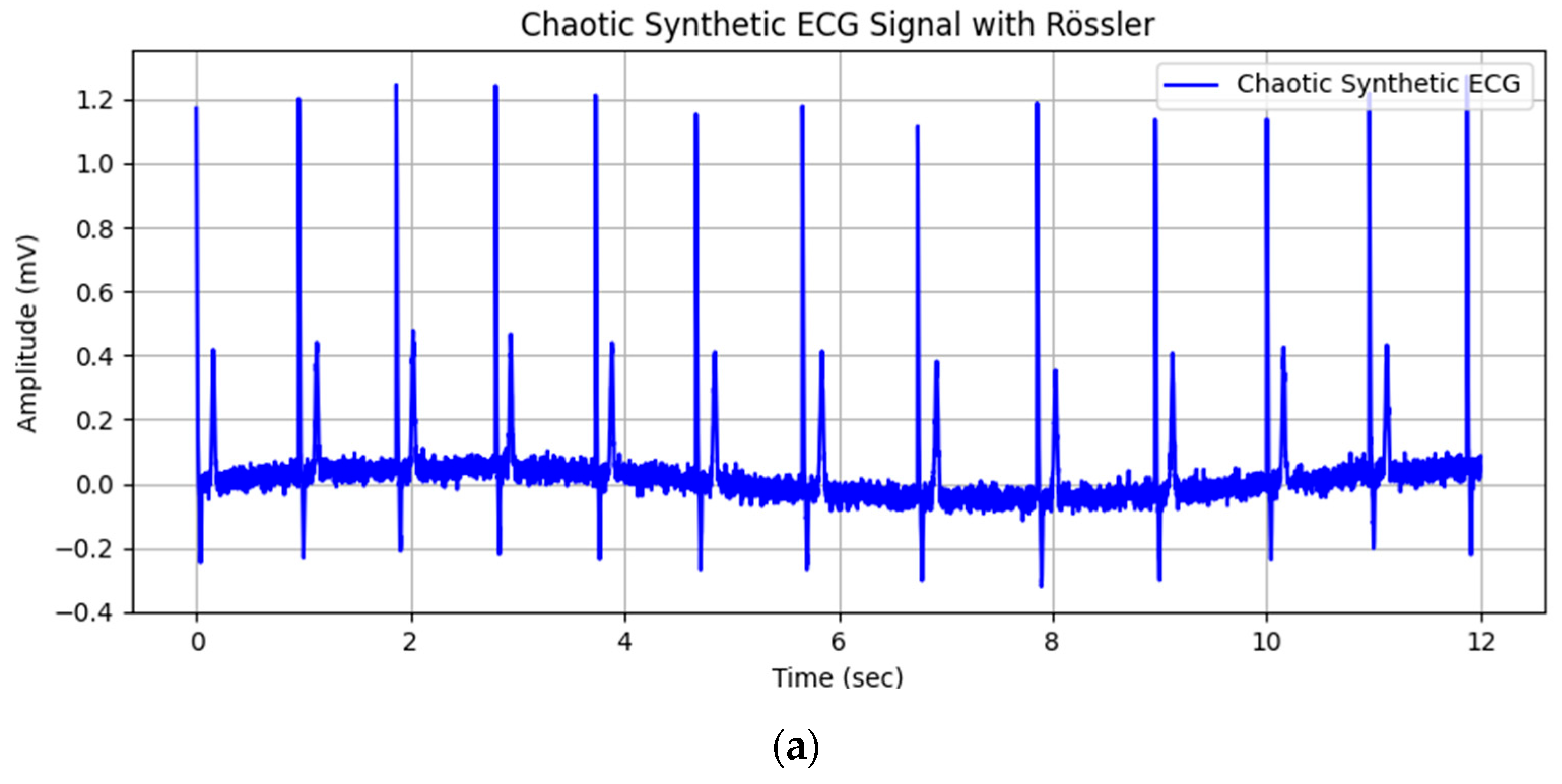
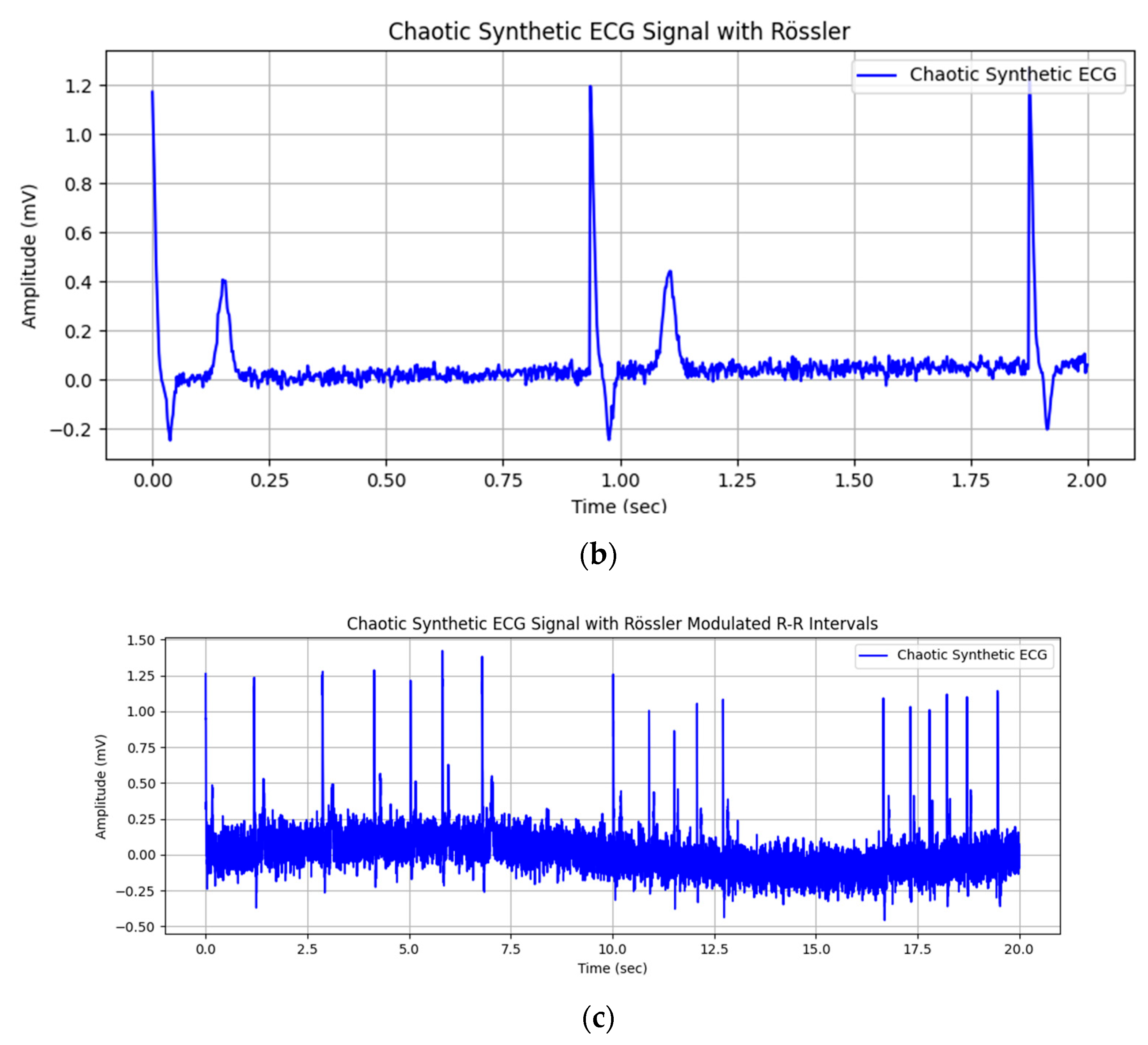
An implementation of a synthetic ECG cycle with an added Rössler attractor to the intervals between R peaks is shown in Figure 6a. In addition to modulating RR intervals, the Rössler attractor can be used to introduce nonlinear dynamics into other features of the ECG signal. This allows for more realistic and complex cardiac simulations. Figure 6b shows two runs of the synthesized signal, where the superimposed noise is generated using Equation (18) and the baseline drift is added using Equation (16). The amplitude of the noise can be adjusted (Figure 6c), allowing flexible control over the simulation parameters to better reflect the variability of real-world ECGs.

Figure 6.
Synthetic ECG cycle with added Rössler attractor to the times between R peaks: (a) With equal distances between pulsations; (b) two cycles of the synthesized signal; (c) with different distances between pulsations and high noise in the ECG baseline.
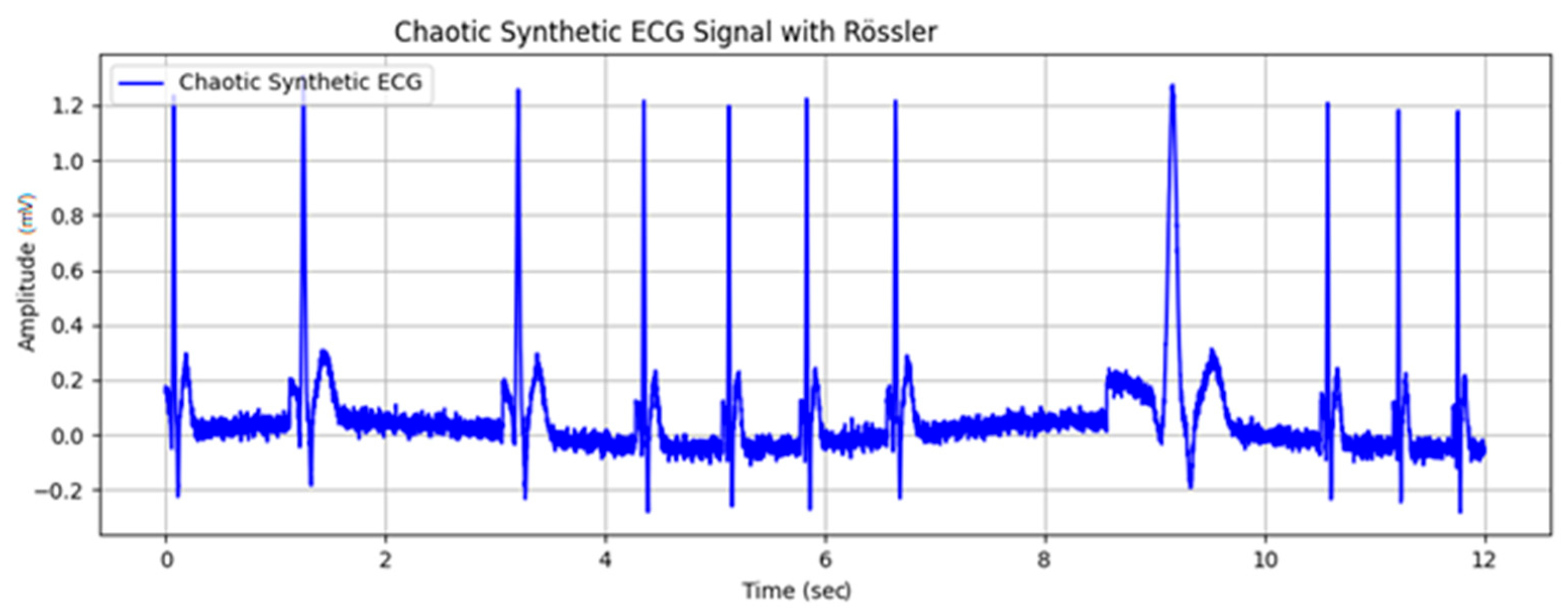
Unevenly distributed time intervals with the capability to simulate irregular pulse and arrhythmia are shown in Figure 7. The irregularity is generated by adjusting the chaotic parameter c in the Rössler attractor system, which directly affects the complexity and variability of the generated dynamics.
Figure 7.
Higher variability in times between adjacent R peaks (adjustable with attractor parameters).
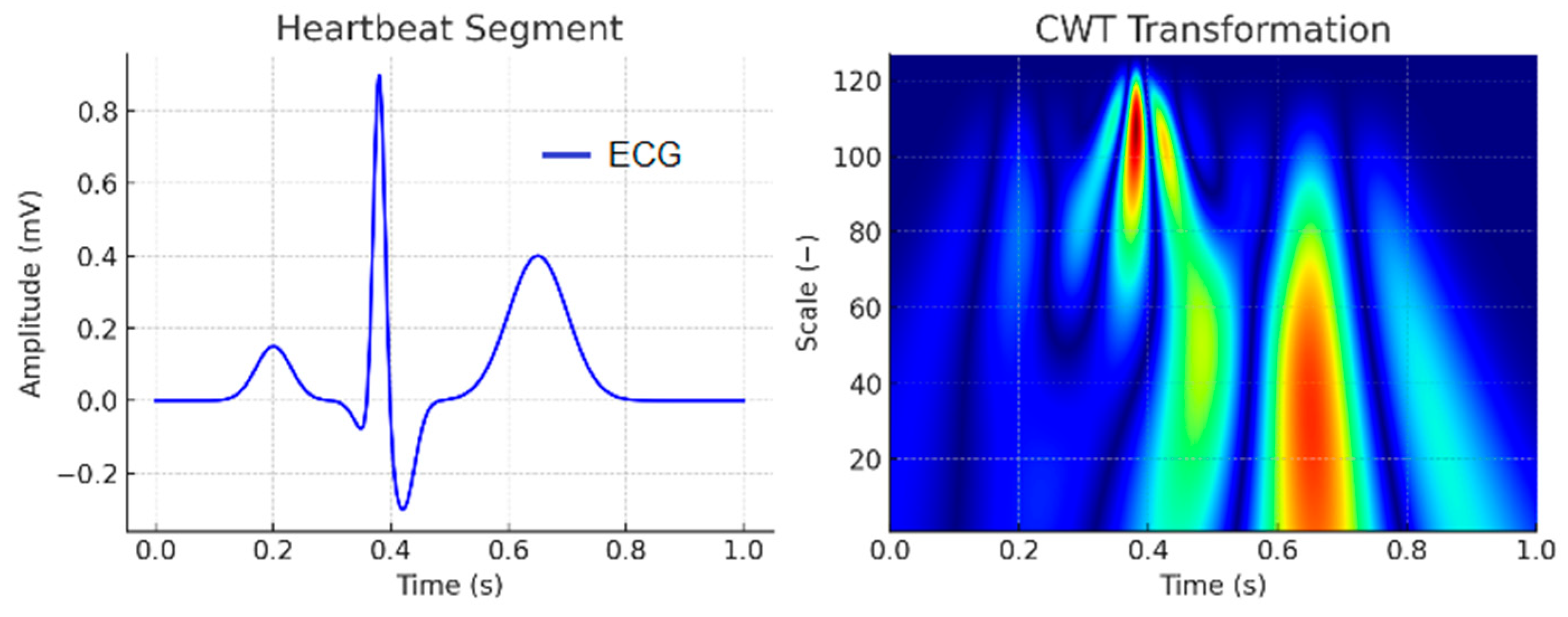
A Continuous Wavelet Transform (CWT) Scalogram was generated to visualize the amplitude of wavelet coefficients as a function of time and frequency scale. The analysis utilized the Mexican Hat wavelet function, which is particularly sensitive to localized rapid changes in the signal, such as those occurring in the QRS complex. The colors in Figure 8 represent the amplitude of the wavelet coefficients, reflecting the signal’s energy concentration at different time points and frequency scales. Red and yellow regions correspond to high-energy components of the signal, typically aligning with the QRS complex and the T wave, which contain the most energy in the ECG. Blue regions indicate low-frequency components and areas with low energy density, such as the P-wave and the segments between heartbeats. This scalogram provides valuable insight into the distribution of frequency components over time, aiding in the analysis of dynamic changes in the ECG signal, including arrhythmias, noise artifacts, and morphological variations.
Figure 8.
CWT scalogram of one heartbeat segment. In the CWT scalogram, the color intensity represents the magnitude of the wavelet coefficients, where warmer colors (yellow–red) indicate higher energy or stronger presence of a frequency component at a given time, while cooler colors (green–blue) correspond to lower energy.
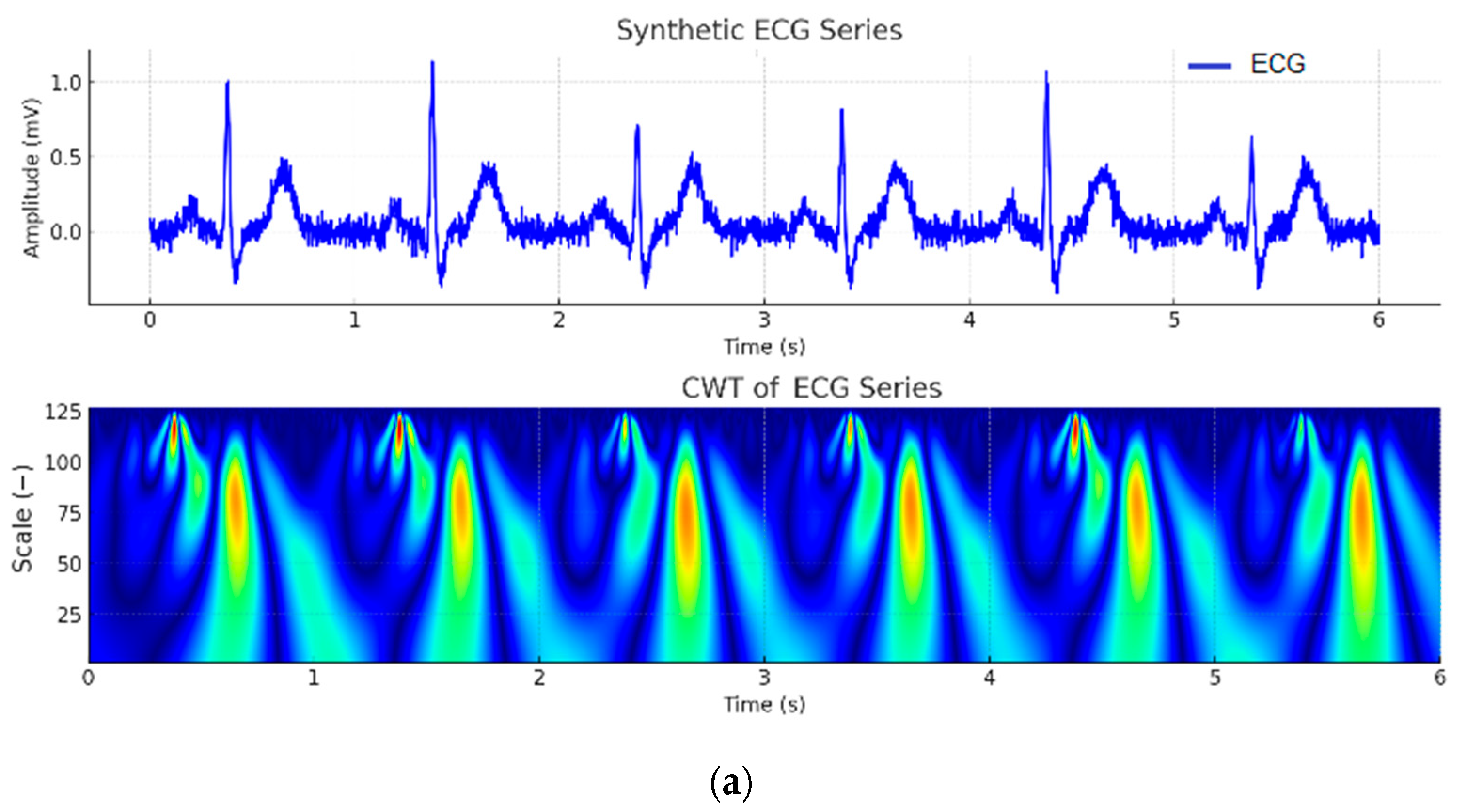
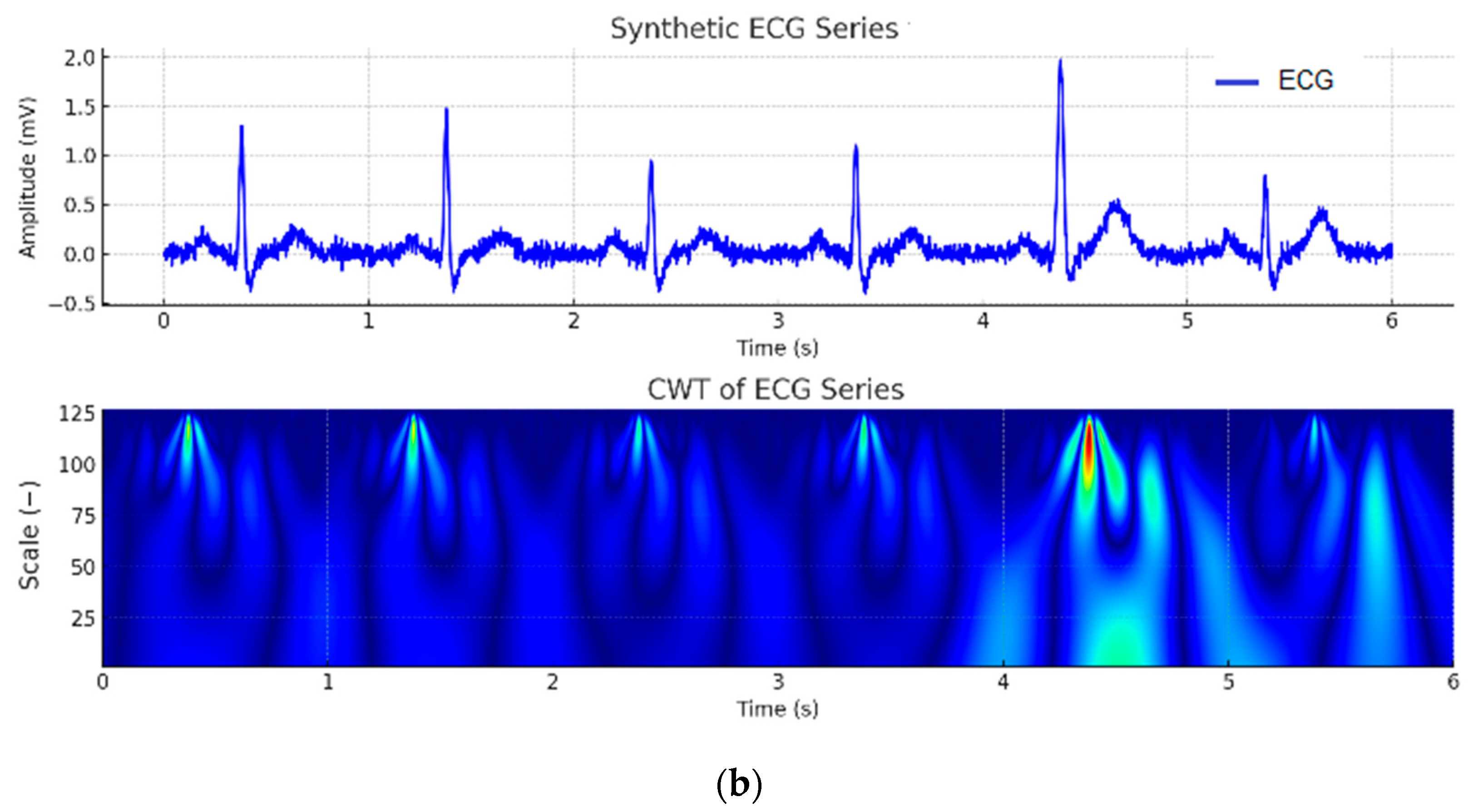
A CWT was applied to an ECG signal with normal R-peak and T wave amplitudes, along with added realistic noise. The graph in Figure 9a highlights regions of high energy (orange and red) at the locations corresponding to the R-peaks and T waves. Figure 9b presents the CWT scalogram of a synthesized interval series characterized by predominantly low R-peaks and weakly expressed T waves. A distinct high-energy short-duration region is observed in the wavelet scalogram at the position of the well-pronounced fifth R-peak, corresponding to its occurrence in the ECG signal. This Figure illustrates the potential for developing frequency-based methods for accurate R-peak localization.

Figure 9.
CWT scalogram: (a) normal RR intervals; (b) a series with small R peaks. In the scalogram, warm colors (yellow–red) indicate high signal energy, and cool colors (green–blue) reflect low energy.
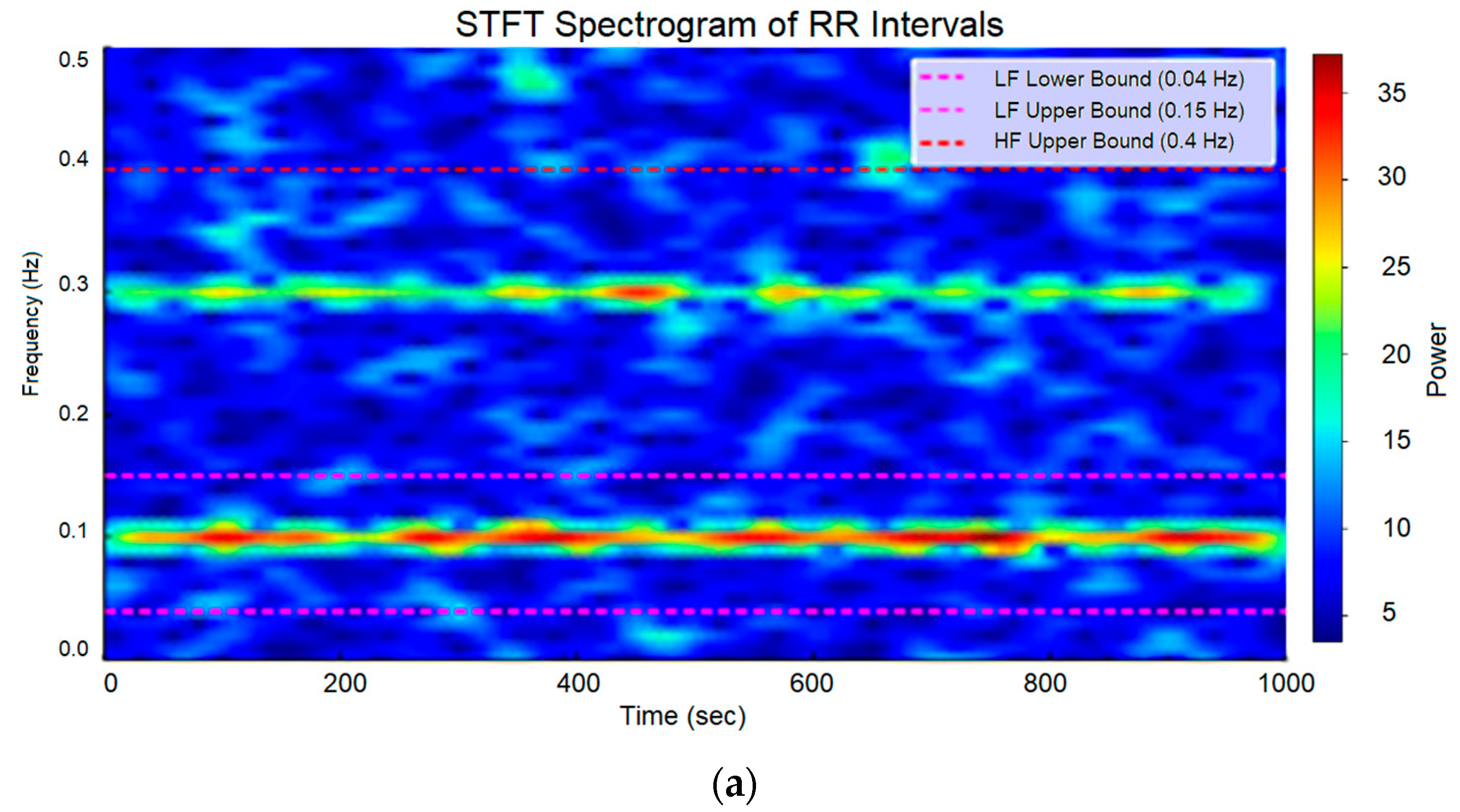
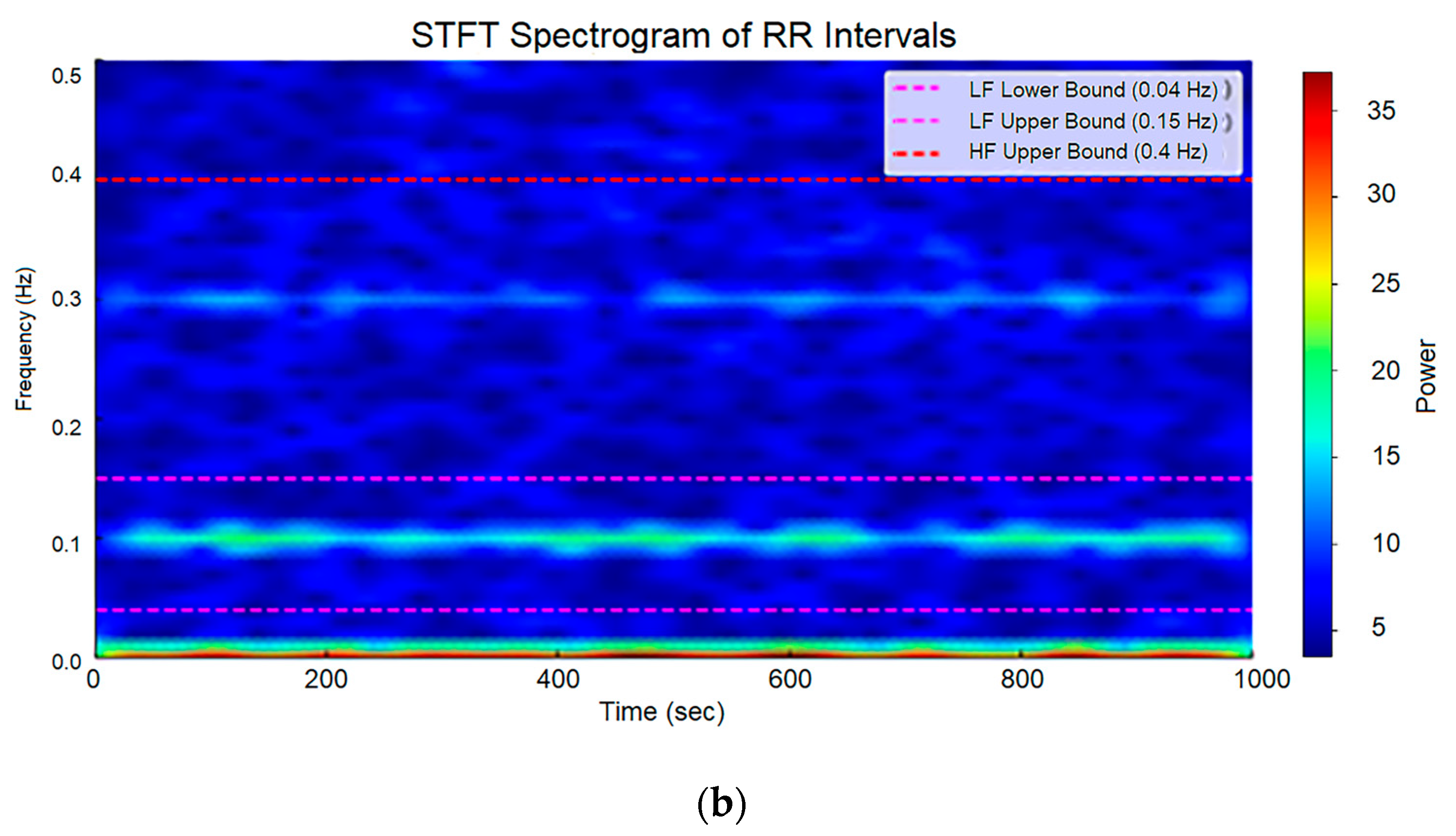
The Short-Time Fourier Transform (STFT) Spectrogram is a time-frequency representation that illustrates how the frequency components of a signal (LF—low frequencies; HF—high frequencies) evolve over time. This is achieved by applying STFT to overlapping time windows, into which the signal is segmented (in this study, a Hann window was used with a window size of 128 intervals, an overlap of 64 intervals, and a sampling frequency of 1 Hz). Within each window, the Fourier Transform is applied to analyze the frequency content of the signal at that specific moment. The result is visualized as a spectrogram, where the X-axis represents time (seconds), the Y-axis represents frequency (Hz), and the color scale indicates the signal amplitude (power of frequency components). Red/yellow areas indicate high energy (strong frequency components), green represents medium energy, and blue indicates low energy or the absence of frequency activity. The STFT spectrogram is particularly useful for analyzing rhythmic and periodic signals, such as cardiac signals. An analysis of the obtained HRV series of RR intervals was conducted using an STFT spectrogram. Figure 10a presents the spectrogram of a generated interval series with normal RR interval variability, while Figure 10b illustrates a spectrogram with low HR variability.

Figure 10.
STFT spectrogram: (a) normal RR intervals (HRV); (b) low HRV.
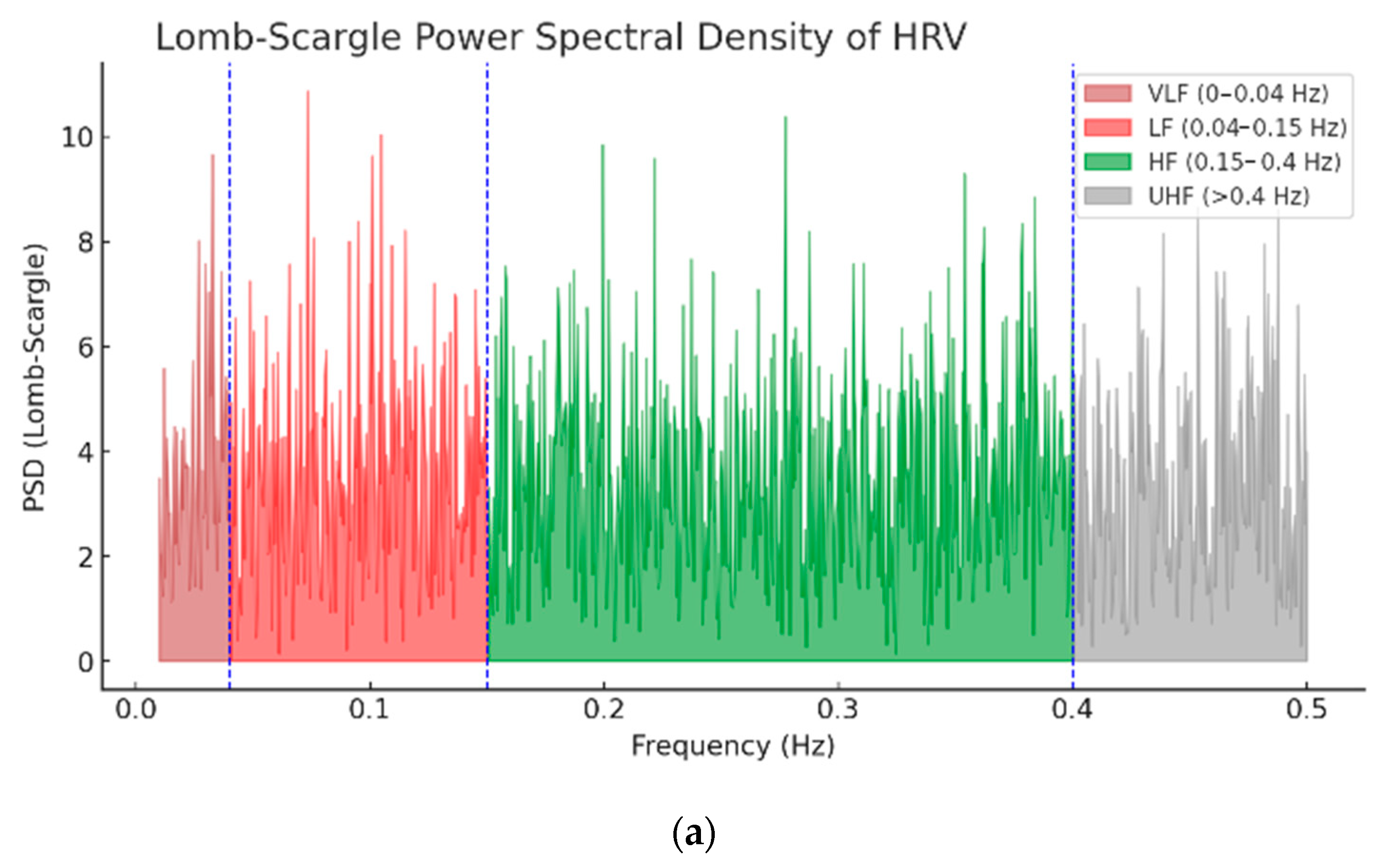
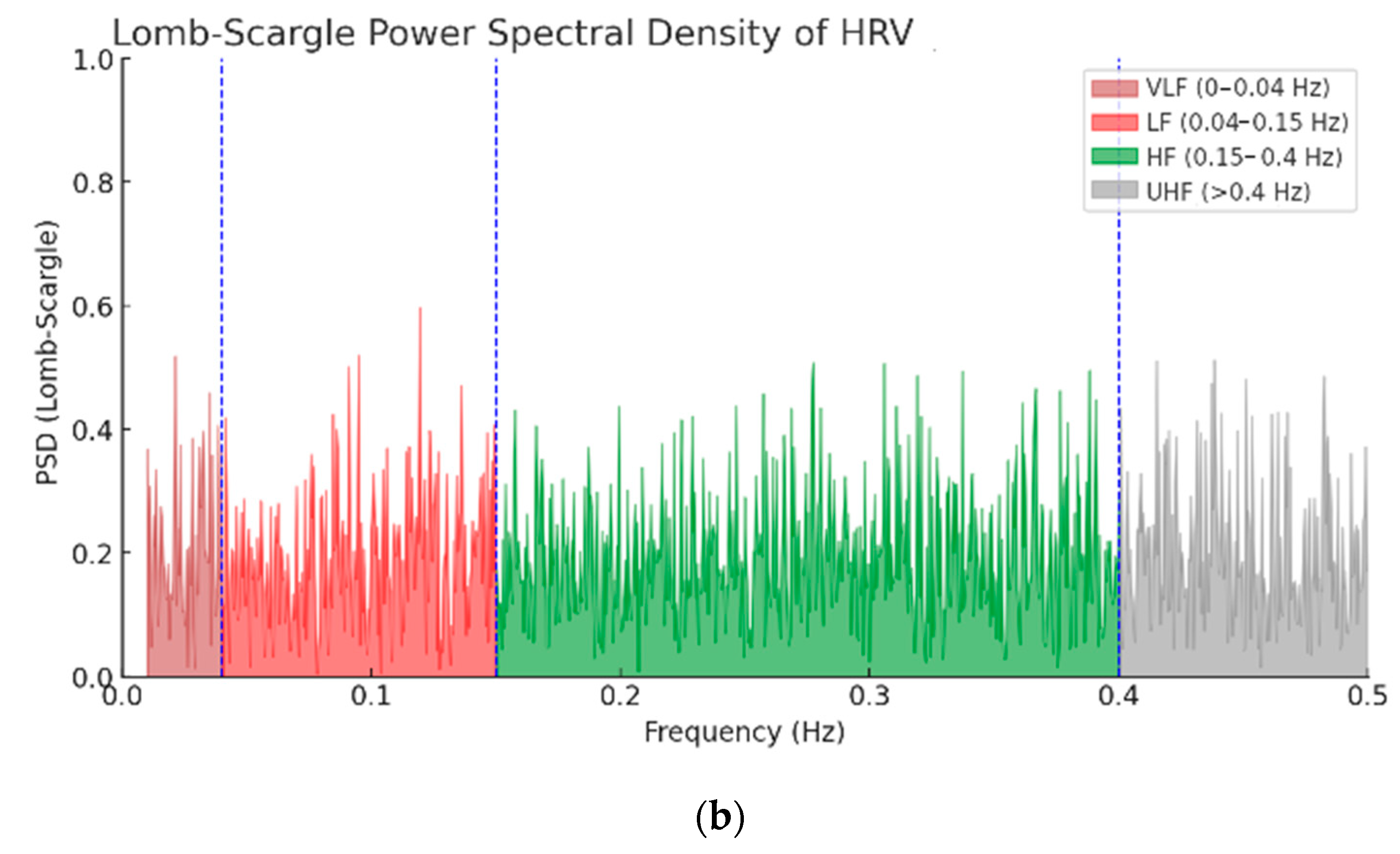
A power spectral density (PSD) analysis of HRV was performed on a synthesized series corresponding to normal sinus rhythm (NSR) (Figure 11a) and on a series with arrhythmic intervals (Figure 11b). In the synthesized series corresponding to NSR, the signal power is significantly higher compared to the non-NSR series (corresponding to an unhealthy cardiac state). The graph also highlights VLF (very low frequency) and UHF (ultra high frequency) areas in addition to the LF and HF components.

Figure 11.
PSD of (a) NSR and (b) non-NSR.
A histogram with a Gaussian distribution corresponding to an ECG series synthesized with normal variability is presented in Figure 12a, while an interval series with irregularly distributed RR intervals is shown in Figure 12b.
Figure 12.
Histogram of ECG beat: (a) Gaussian distribution; and (b) non-Gaussian distribution.
For the analysis and testing of the presented algorithm, a Python program was developed.
The results for the calculated HRV parameters in a simulated cardiac series corresponding to a healthy individual (normal variability in the interval time series) are presented in Table 3. The parameters for a real ECG with NSR are also shown. Both types of examined series have a duration of 30 min, with the results averaged over 12 series. The HRV parameter values of the synthesized series fall within the normal range for NSR, indicating that the proposed method can generate realistic cardiac series for healthy individuals. The conducted t-test confirms that there are no statistically significant differences between the HRV parameters of the two types of series.
Table 3.
Comparison of HRV parameters between real and simulated ECG signals with normal sinus rhythm.
Arrhythmia/healthy recordings were obtained with a Holter at the Medical University of Varna, Bulgaria, under the supervision of a cardiologist.
The simulation of series with significant arrhythmic variability can be used for studying ECG series with non-normal sinus rhythm (e.g., arrhythmia). The results of the HRV analysis for 12 real ECG series with arrhythmia and 12 synthesized ECG series with arrhythmic beats are presented in Table 4. The conducted t-test demonstrates that the HRV parameters of both series do not show statistically significant differences, indicating that the proposed algorithm can effectively generate ECG series with arrhythmic beats.
Table 4.
HRV results for real and simulated ECG with arrhythmia (heart rhythm disorder).
Table 5 quantitatively summarizes all key HRV parameters for real and simulated ECG signals in three physiological states: rest, fatigue, and stress. Time (MeanRR, SDNN, and RMSSD), spectral (TP, nLF, nHF, and LF/HF), and nonlinear (Hurst, SampEn) parameters are included with the corresponding 95% confidence intervals. The table allows a direct comparison between real and simulated signals and shows how different states affect heart rate variability. The frequency parameters, nLF, nHF, LF/HF, and TP are calculated using power spectral density (PSD). They show the distribution of energy in the low- and high-frequency bands and the total power of the HRV signal. Comparing real and simulated signals, it is seen that PSD allows a quantitative assessment of autonomic regulation and adaptation of heart rate in different states.
Table 5.
Comparison of HRV parameters between real and simulated signals for three physiological states: rest, fatigue, and stress.
Across all HRV parameters, the effect sizes between real and simulated data remained predominantly small, with |d| < 0.5 in almost all comparisons (Table 6). For the rest and fatigue states, the vast majority of effect sizes fell in the negligible-to-small range, indicating close agreement between real and synthetic distributions. In the stress condition, several parameters showed moderate effects (e.g., SD2/SD1), reflecting the increased physiological variability and reduced stationarity typical for post-competition recordings. Importantly, the sign of d only indicates direction (real > simulated or vice versa), while the consistently low magnitude confirms that the proposed model reproduces HRV behavior with high fidelity across all physiological states.
Table 6.
Statistical comparison (p-values and Pearson correlation) between real and simulated signals—HRV parameters across rest, fatigue, and stress states.
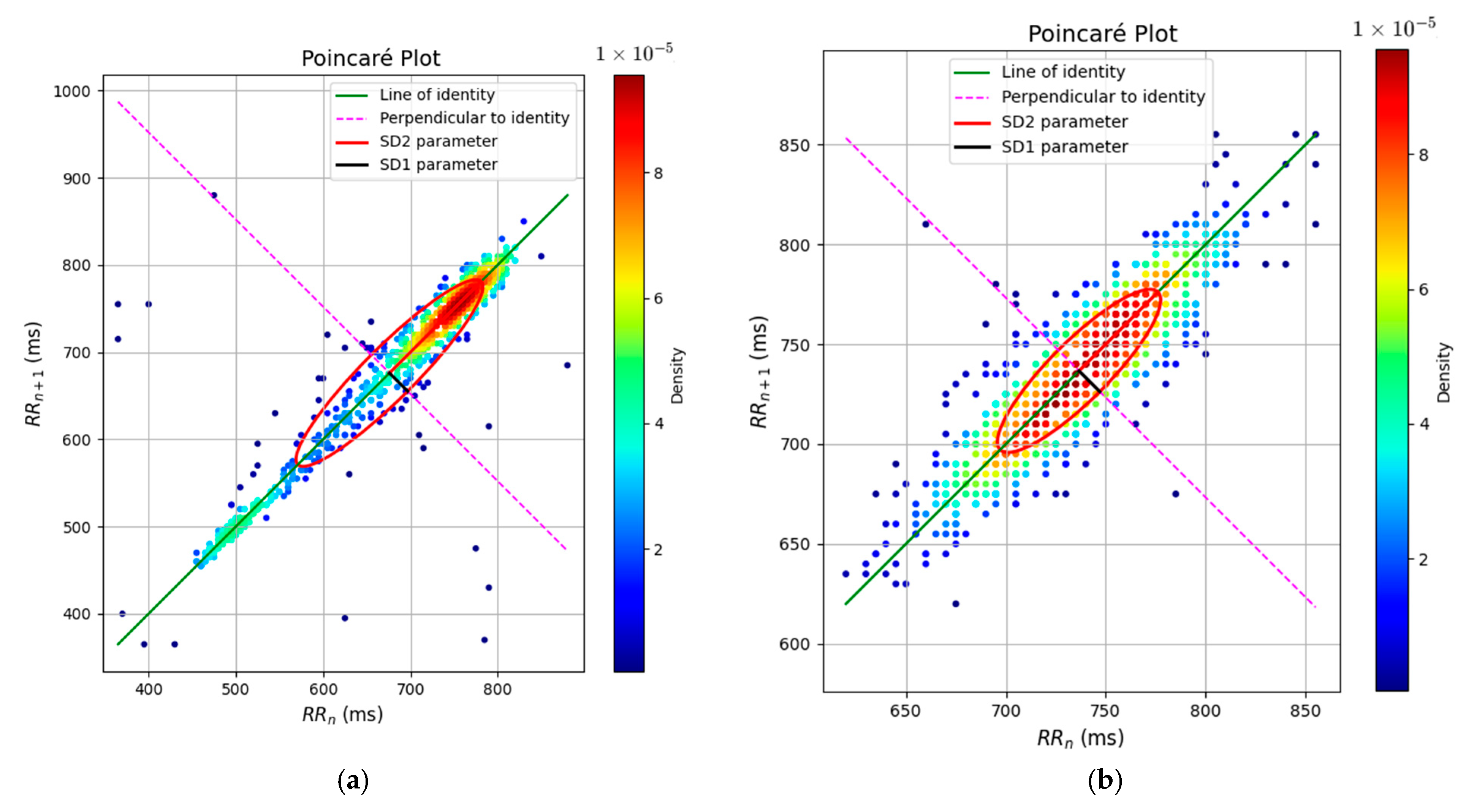
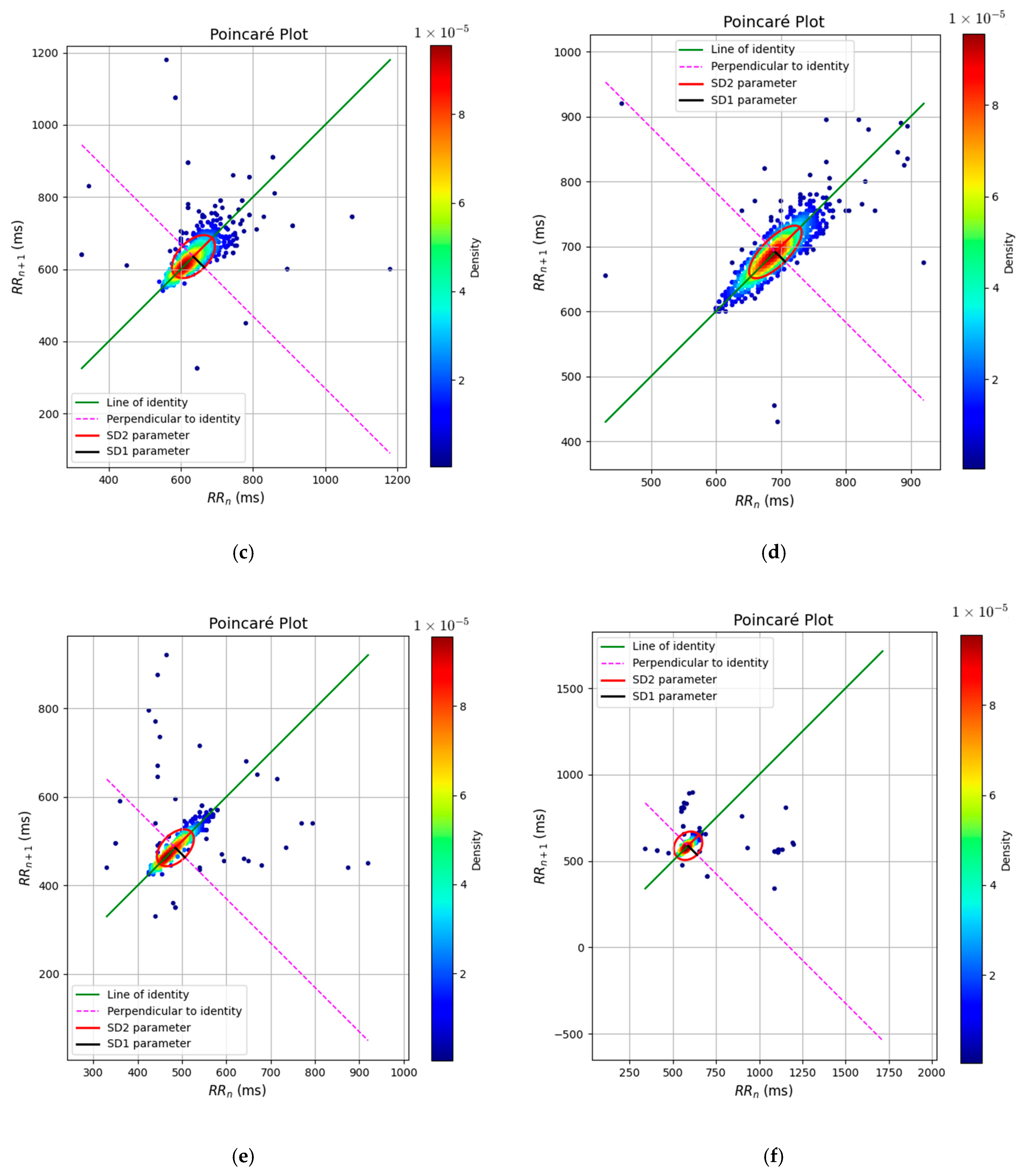
Poincaré plots parameters (Table 7). The SD1, SD2, and SD2/SD1 indices demonstrate close values between the real and simulated RR intervals in all physiological states, with overlapping 95% confidence intervals. In all three states, the model reproduces the characteristic trends—a decrease in SD1 and SD2 from rest to fatigue and stress, as well as an increase in SD2/SD1, which reflects increased sympathetic dominance. The high correlations (0.72–0.86) and small effect sizes (Table 8) indicate that the differences between real and synthetic data are minimal.
Table 7.
Poincaré plots parameters for real and simulated signals across rest, fatigue, and stress conditions.
Table 8.
Statistical comparison between real and simulated signals—Poincaré plots parameters across physiological states (rest, fatigue, and stress).
Figure 13 presents the Poincaré plots for real and simulated ECG-derived RR intervals under three physiological states: rest, fatigue, and stress. The characteristic ellipsoidal patterns reveal a progressive reduction in HRV with increasing physiological load. In both real and simulated data, the dispersion of points along the line of identity (SD2) and the perpendicular direction (SD1) decreases notably from rest to stress, reflecting diminished long- and short-term variability, respectively. The simulated plots (b, d, f) closely replicate the morphology and orientation of the real data (a, c, e), confirming that the attractor-based model successfully captures the nonlinear dynamics of autonomic modulation across different conditions. The narrowing of the ellipse and the increased point density in the stress condition indicate a shift toward sympathetic dominance, consistent with the elevated LF/HF ratios observed.

Figure 13.
Poincare Plot: (a) Rest real; (b) rest sim; (c) fatigue real; (d) fatigue sim; (e) stress real; and (f) stress sim.
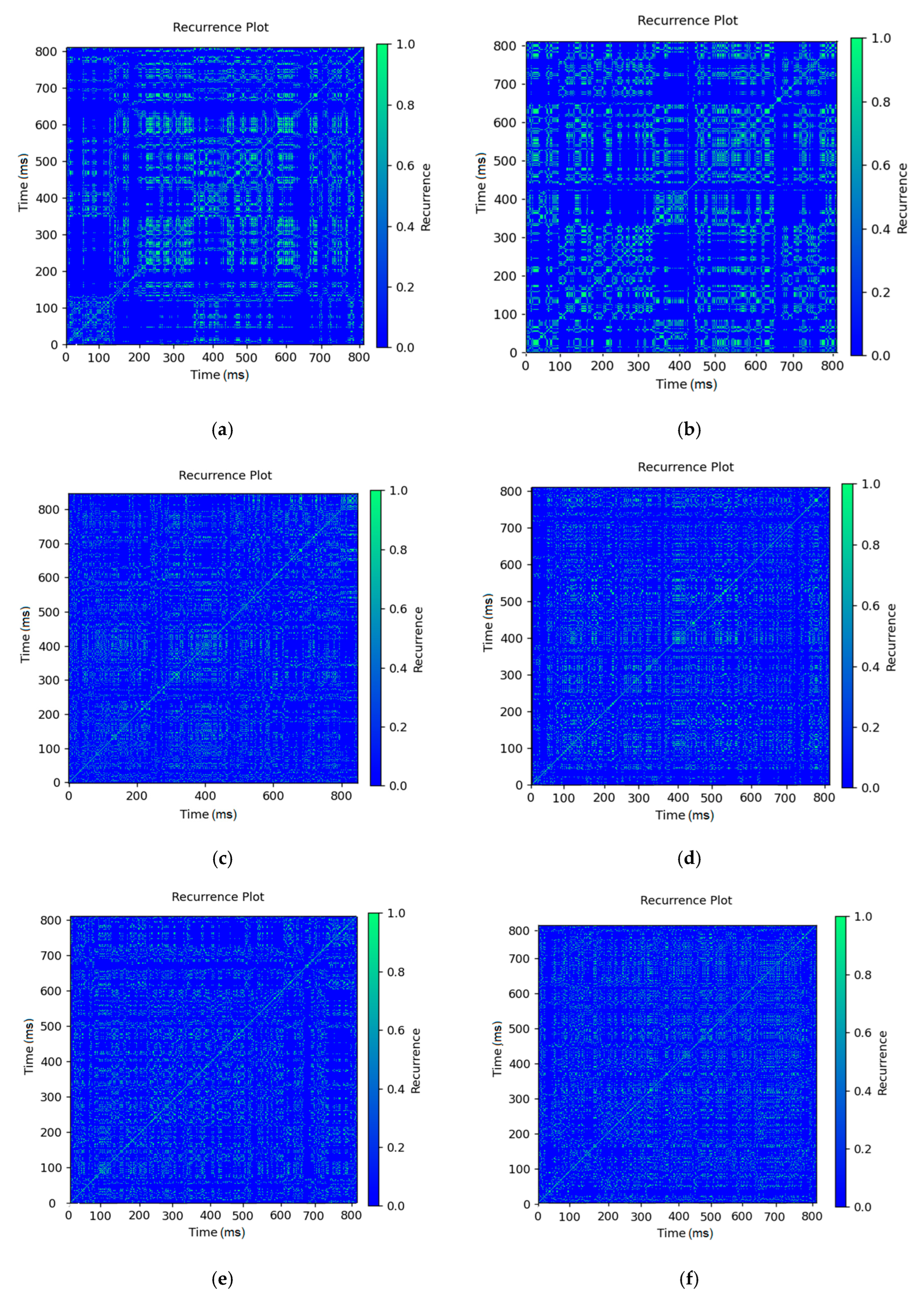
Recurrence plot indices (Table 9). The RQA metrics demonstrate almost identical values between the real and simulated signals in all physiological states. REC, DET, and LAM follow the same trends in rest/fatigue/stress, indicating that the model accurately reproduces the increasing complexity and decreasing resilience of the system under physiological stress. The maximum linearity (Lmax), Trapping Time, and the entropy ENTR also show very close mean values and overlapping 95% confidence intervals, further confirming the coincidence in the dynamic structure of the phase space. The statistical test (Table 10), high correlations (0.75–0.83), and small effect sizes (|d| < 0.25) indicate that the differences between the real and generated signals are not significant.
Table 9.
Recurrence plot indices for real and simulated signals across rest, fatigue, and stress conditions.
Table 10.
Statistical comparison between real and simulated signals—recurrence plot indices across physiological states (rest, fatigue, and stress).
Figure 14 visualizes the recurrence plot (RP) of the RR intervals in the three physiological states—rest, fatigue, and stress—for both real (Figure 14a,c,e) and simulated Figure 14b,d,f signals. Each of the RPs was obtained by calculating the pairs of time points with similar amplitude of the intervals, at a fixed proximity threshold. In the rest state (Figure 14a,b), both the real and simulated signals show a distinct structural periodicity, with clearly defined diagonal and secondary lines—an indication of strong regularity and high HRV. In fatigue (Figure 14c,d), the RPs retain some structure, but with less clarity—this reflects reduced variability, but still existing internal coherence of the heart rhythm. In the stress state (Figure 14e,f), the RPs demonstrate a more chaotic structure, with reduced symmetry and fragmentation of the repeating structures. This indicates a significant decrease in HRV and higher entropy—a marker of autonomic nervous system dysregulation. Therefore, the simulation model successfully captures not only the quantitative but also the geometric properties of the temporal dynamics of the heart rate.
Figure 14.
Recurrence plot: (a) Rest real; (b) rest sim; (c) fatigue real; (d) fatigue sim; (e) stress real; and (f) stress sim.
Table 11 and Table 12 summarize a quantitative comparison between real and simulated HRV signals using key nonlinear metrics of three-dimensional phase attractors. The metrics include Lyapunov λ1, Correlation Dimension D2, and Permutation Entropy, and present mean values, confidence intervals, statistical significance (p-value), correlation, and effect size for the three physiological states: rest, fatigue, and stress. The tables demonstrate that the simulated signals successfully reproduce the complex dynamics of HRV, quantitatively approaching the real signals.
Table 11.
Three-dimensional phase space attractor metrics for real and simulated HRV signals across rest, fatigue, and stress conditions.
Table 12.
Statistical comparison between real and simulated nonlinear HRV metrics for a three-dimensional phase space attractor across physiological states (rest, fatigue, and stress).
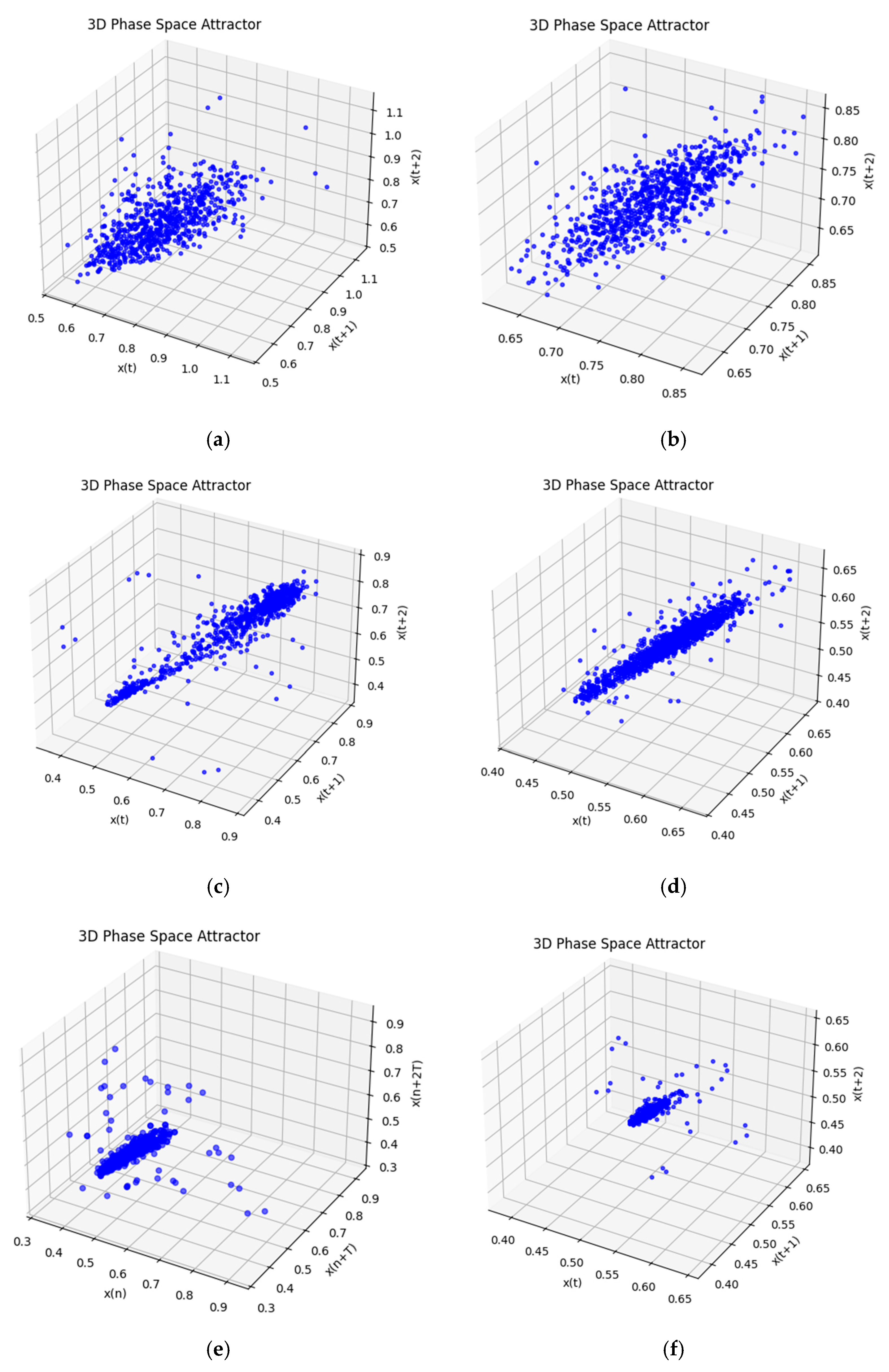
Figure 15 presents three-dimensional phase space attractors generated from real and simulated HRV signals in three physiological states: rest (Figure 15a,b), fatigue (Figure 15c,d), and stress (Figure 15e,f). The attractors are constructed by time-delayed embedding of RR intervals, (t), (t + 1), x(t + 2), in order to visualize the geometric structure and dynamics of the signal. In the rest state, Figure 15a,b, a broad but compact ellipsoidal shape is observed, reflecting normal, non-chaotic variability. The simulated data (Figure 15b) successfully reproduces the volume and shape of the real attractor, Figure 15a, with a moderate density of points. In the fatigue state, Figure 15c,d, the attractors are drawn diagonally and demonstrate higher linear coherence, which indicates reduced signal complexity. The simulation (Figure 15d) reproduces this effect with good accuracy. Under stress (Figure 15e,f), a clear narrowing and compression of the attractor is observed, indicating increased regularity and reduced dynamics—characteristic of sympathetic dominance. The simulation (Figure 15f) manages to capture the main features, although with a slight underestimation of the volume and scattering of the points.
Figure 15.
Three-dimensional phase space attractor: (a) Rest real; (b) rest sim; (c) fatigue real; (d) fatigue sim; (e) stress real; and (f) stress sim.
The 36 simulated RR time series generated for each physiological state were compared with the 36 corresponding real RR series using a one-to-one index-based pairing (i.e., real series i was compared with simulated series i). This approach ensures equal sample sizes and preserves the statistical structure of each physiological state. RMSE quantified amplitude deviation, while DTW measured temporal similarity between each real and synthetic pair (Table 13). Low RMSE values across all groups indicate small point-wise errors between real and synthetic RR dynamics, while the moderate-to-low DTW distances confirm that the simulated sequences successfully reproduce the temporal structure of physiological HRV. Together, these metrics provide a stronger validation of equivalence than correlation alone, addressing the reviewer’s concern regarding the adequacy of the validation methodology.
Table 13.
RMSE and DTW similarity metrics between real and simulated RR-interval time series across rest, fatigue, and stress states.
In addition to the RR-interval analysis, similarity at the waveform level was also assessed.
For normal heart rhythm (for real signals) and physiological resting state (for simulated signals), an averaged PQRST template was extracted from the real ECG and the corresponding simulated ECG. To quantitatively assess the morphological similarity between real and synthetic QRS complexes, we performed an analysis on normal beats (AAMI class N) from the MIT-BIH Arrhythmia Database. Only morphologically stable normal beats were used; after R-peak alignment, resampling to 256 points, and amplitude normalization, N = 120 beats were constructed, from which we obtained a Statistically Averaged Beat (SAB) as a reference template. Each synthetic QRS generated by the chaotically modulated Rössler model was compared to the SAB using DTW, Pearson correlation, and normalized root mean square error (NRMSE).
The obtained results showed that the average waveform correlation exceeded r = 0.90, DTW distances remained low (<9.2), and NRMSE was low (<0.2), which confirms that the proposed morphological model reproduces the shape and timing of physiological P, QRS, and T waves and the reviewer’s request for validation at the waveform level well.
The results for ECG cycle generation time are presented in Table 14. The CPU time measurements were performed using an Intel(R) CoreTM i3-8100 CPU, 3.60 GHz. Table 6 presents the CPU time required for ECG cycle generation with different numbers of RR intervals. The computational experiments were conducted on an Intel(R) Core™ i3-8100 CPU at 3.60 GHz. The obtained results show that the CPU time increases proportionally with the number of RR intervals. A linear regression analysis yielded a high coefficient of determination (R2 ≈ 0.99), confirming that the relationship between computation time and input size is nearly linear. Therefore, the computational complexity of the ECG cycle generation algorithm can be approximated as O(N), where N is the number of generated RR intervals. This indicates efficient scalability of the implementation, as no evidence of exponential or quadratic growth (O(N2) or O(eN)) was observed, even for large data sizes up to 900,000 samples.
Table 14.
CPU time as a function of the number of generated RR intervals.
- Computational Complexity Analysis
The computational complexity of the proposed hybrid ECG generation algorithm consists of two sequential components:
- (1)
- Numerical integration of the Rössler attractor using the fourth-order Runge–Kutta (RK4) method;
- (2)
- Beat-wise synthesis of the ECG morphology using Gaussian mesa functions (GMFs).
The Rössler system Equation (4) is integrated with step size Δt over the simulation horizon T.
The RK4 update is as follows:
where each ) requires a constant number of arithmetic operations.
The number of RK4 iterations is as follows:
and the total number of generated RR intervals is proportional to , and therefore we obtain the following:
Each heartbeat k = 1,…,N is synthesized using the GMF-based waveform model with Equation (12).
Each GMF component requires a constant number of exponential and arithmetic operations. With = 5 wave components, the synthesis cost is as follows:
Since the integration and synthesis stages are executed sequentially, we have the following:
Thus, the entire ECG generation algorithm scales linearly with the number of heartbeats.
4. Discussion
Recent advances in fractional and chaotic modeling emphasize the need for hybrid, physiologically grounded simulators. For example, ref. [48] proposed novel Newton-interpolation-based schemes for fractal–fractional biomedical dynamics, illustrating the growing impact of non-integer calculus in physiology. Our hybrid Gaussian–Rössler framework complements this trend by coupling chaotic HRV modulation with explicit ECG morphology, while keeping linear-time complexity against classical dynamical ECG generators.
The comparative analysis presented in Table 15 covers studies in the field of ECG signal synthesis using Gaussian functions. Most authors use a fixed number of GDF, usually between 2 and 8, and specify three parameters per waveform (amplitude, width, and position), which corresponds to the classical model introduced by McSharry et al. The following limitations are noted in the analyzed works: Lack of variability—although the waveform shape is well controlled, most models do not incorporate HRV or realistic variations between RR intervals. This limits their applicability in simulations of physiological states. Lack of attractor dynamics—none of the studies employ phase space attractors or chaotic models to control the variability of RR intervals, which leads to linear and repetitive structures. Computational efficiency—only [7] documents CPU performance; the remaining works do not evaluate computational cost.
Table 15.
Overview of ECG signal synthesis studies using Gaussian functions.
The current approach introduces several new elements that extend the capabilities of GDF-based synthesizers: Adaptive number of Gaussian functions: six basic GMFs are used, with the possibility of adding additional components (e.g., baseline waves, noise, and baseline drift), which allows for more flexible modeling. Extended parametric model: five parameters are used for each Gaussian wave and seven parameters for the attractor structure, which provides more realistic morphology and dynamics. Generation of HRV through phase space attractors—this allows for the creation of signals with different states (rest, fatigue, and stress), mimicking real physiological dynamics. CPU load evaluation—the efficiency of the algorithm is evaluated, including simulation time and resource consumption, which makes it suitable for embedded and edge systems.
The compact representation of the fundamental waves of the ECG signal through fewer functions facilitates the modeling of ECG morphology, but is not sufficient to capture the complex variability observed in physiological cardiac signals.
The proposed model uses five Gaussian parameters in the waveform generator (GMF), together with a 7-parameter attractor variability module. This allows not only accurate modeling of P, Q, R, S, and T waves, but also introduces controlled variation in amplitude, width, and baseline shift over time—features critical for mimicking the real behavior of HRV under different physiological states (rest, fatigue, and stress). While earlier models are usually static and do not model HRV fluctuations, the proposed approach integrates an attractor-driven modulation mechanism that introduces nonlinear and time-evolving HRV profiles. This provides a more realistic simulation framework for AI-based ECG classifiers, wearable device testing, and digital twin environments. This approach, combining a generative ECG morphology module with a dynamically tunable attractor model, enables the synthesis of realistic transitions between physiological states. The proposed model is designed to be computationally efficient and compatible with embedded platforms, allowing its use in resource-constrained environments, such as wearable devices and simulated patient monitors, and can serve as an AI training tool. The extended parameterization supports the simulation of noisy or pathological models, allowing the generation of abnormal ECG cases, motion artifacts, or signal distortions for stress-testing of detection algorithms. The adjustable number of Gaussians in the method allows for flexible adaptation to different ECG morphologies or synthetic pathologies. Six features are sufficient to model the canonical waveform structure, but the framework allows for the addition of more components (e.g., premature complexes) if necessary for realistic modeling of cardiac pathologies.
Comparison of the Three Synthetic ECG Models Against Normal HRV Physiology.
A comparison of the presented model with the McSharry and Zeeman models is made.
Some general points about the McSharry model and the Zeeman model.
A synthetic ECG signal is generated by the McSharry model. The signal is generated by a set of differential equations that describe the phase dynamics of the heart rhythm. The basic model uses a three-dimensional phase attractor, where the phase θ governs the sequence of P, QRS, and T waves, and the amplitude and morphology of the waves are modeled by phase functions. The equations include the phase velocity and Gaussian functions for the individual waves, and their integration over time produces a synthetic ECG signal. The built-in attractor is located in the 3D phase space (x, y, z), where x and y define the circular trajectory, and z defines the morphology of the wave, providing a continuous and stable simulation of the cardiac cycle.
In ECG synthesis with the Zeeman model, the signal is generated by nonlinear differential equations that describe the phase dynamics of the heart rhythm and the morphology of the waves. The model includes parameterization of the P, QRS, and T waves by functions of phase and amplitude, introducing inertial and recovery terms to simulate realistic variations in the RR intervals. The built-in attractor is present in the three-dimensional phase space, where the coordinates determine the phase, amplitude, and morphological characteristics of the waves, providing a stable trajectory of the cardiac cycle and the ability to control the variability of the synthesized ECG. The integration of this system over time produces a smooth three-dimensional trajectory, which is a built-in attractor reflecting the repeatability and dynamics of the cardiac cycle. Thus, the model allows for the controlled generation of realistic ECG signals with the ability to modulate the variability and morphology.
The comparison of the three models was conducted under the same input conditions:
- Sampling frequency (fs): 500 Hz.
- Recording duration: 5 min (300 s).
- Average heart rate (HRmean): 60 bpm (1 Hz).
- Gaussian noise level: 0.03.
- Low-frequency modulation: 0.05 (for resting state).
- Baseline/Drift: amplitude 0.11, and frequency 0.04 Hz (simulates slow variations).
- McSharry and Zeeman: Ordinary differential equation parameters according to the original models, no change, and only amplitude scaling for benchmarking.
These values are identical for all three models to ensure a horizontal comparison at a resting heart rate, without the influence of extreme physiological variations.
The comparison shows differences between the three models (Table 16) in terms of how realistically they reproduce the temporal, spectral, and nonlinear HRV characteristics observed in normal sinus rhythm.
Table 16.
Comparison of HRV metrics between normal physiology and the three synthetic ECG models.
The McSharry model reproduces normal variability well, in general, but overestimates short-term HRV (RMSSD 45.9 ms; pNN50 ≈ 30%), resulting in an increased parasympathetic component. The LF component (1846 ms2) is elevated, and LF/HF = 2.78 is higher than the typical range of 1.5–2.0. Furthermore, SD1/SD2 = 0.32 indicates a strong longitudinal dominance.
The HRV parameters according to the Zeeman model show a deviation from the norm. SDNN (212 ms) and total power (~7256 ms2) are more than twice the physiological values, LF is extremely elevated (5892 ms2), as is HF (1353 ms2), resulting in a very high LF/HF = 4.29. Nonlinear Poincaré metrics (SD1/SD2 = 1.24) show an atypical circular shape of the attractor, characteristic of highly turbulent or non-physiologically generated RR series.
The Gauss–Rössler model is closest to the physiological values. SDNN (131.8 ms), total power (≈2680 ms2), LF (1429 ms2), HF (1007 ms2), and LF/HF (1.42) fall within the range of normal autonomic modulation. The ratio SD1/SD2 = 0.69 is also realistic and corresponds to healthy young individuals with balanced vagal and sympathetic tone.
In summary, the Gauss–Rössler model shows a good fit to normal HRV physiology, reproducing adequate values for SDNN, SDANN, RMSSD, pNN50, total power, LF/HF, and Poincaré parameters. The McSharry model partially reproduces normal variability but exaggerates parasympathetic activity. The Zeeman model fails to achieve a realistic distribution of HRV components and generates excessively high variability. However, it should be noted that the comparison made is based on 12 generated 5 min series from each model, which is a significant limitation. A plausible comparison between the three models requires extensive and long-term studies, which could be the subject of future work.
While earlier ECG synthesis models are predominantly static and do not account for the intrinsic fluctuations observed in heart rate variability (HRV), the proposed hybrid framework introduces an attractor-driven modulation mechanism capable of generating nonlinear, time-evolving RR-interval dynamics. This is clinically relevant because HRV is strongly associated with autonomic nervous system (ANS) regulation and serves as a biomarker for a broad range of cardiovascular and systemic conditions, including stress, heart failure, arrhythmia susceptibility, and post-exercise recovery [53].
By simulating physiologically plausible transitions between rest, fatigue, and stress states, the model can be used to evaluate algorithms that depend on such dynamic signatures.
From the perspective of artificial intelligence, realistic synthetic ECG and HRV data are increasingly required for data augmentation, domain adaptation, and training of deep learning models, particularly when real annotated datasets are limited or protected by privacy regulations. Recent studies demonstrate that generative synthetic ECG signals can significantly improve classifier robustness and reduce overfitting in arrhythmia detection systems [54]. The ability of the proposed model to incorporate controlled levels of noise, motion artifacts, baseline wander, and amplitude modulation makes it suitable for creating stress-test scenarios for both classical signal-processing and machine learning pipelines.
Additionally, the model’s compatibility with embedded and low-power platforms is beneficial for contemporary wearable health-monitoring technologies. Modern wearables rely heavily on real-time ECG reconstruction, HRV estimation, and artifact suppression, yet are constrained by limited computational resources. Lightweight generative models have been shown to improve on-device learning and calibration for personalized monitoring [55]. The computational efficiency of the present framework (linear complexity O(N)) allows for its integration into wearable firmware, enabling on-device simulation, data augmentation, or validation during firmware or sensor design.
Clinically, the ability to generate abnormal ECG morphologies—such as attenuated R-peaks, ectopic beats, prolonged QRS complexes, or T wave alternans—offers strong potential for controlled simulation of pathological states without exposing patients to risk. Synthetic—but physiologically meaningful—arrhythmias can be used to pre-train or stress-test diagnostic algorithms, improving generalization to rare, dangerous events such as ventricular tachycardia or atrial fibrillation. This aligns with ongoing efforts toward digital twin modeling in cardiology, where individualized virtual patients are used for predictive modeling and treatment optimization [37].
Finally, the adjustable number and parametrization of GMF components allow the framework to cover a broad morphological spectrum. While six Gaussian mesa functions are sufficient to reproduce canonical ECG cycles, additional components—such as premature atrial/ventricular contractions, ST-segment deviations, or repolarization abnormalities—can be incorporated to model specific clinical scenarios. This extensibility makes the method suitable not only for synthetic signal generation but also for algorithm benchmarking, computational physiology research, and multi-modal AI systems for cardiology.
Limitations.
Although the attractor-based variability mechanism captures basic HRV patterns across physiological states, it remains a deterministic module and may not fully emulate the stochasticity observed in HRV dynamics, e.g., in pathological states such as atrial fibrillation.
The present evaluation was limited to three physiological states (rest, fatigue, and stress) and two medical states: healthy and arrhythmia. Although the system supports parameter flexibility, its generalizability to other states (e.g., sleep apnea, ischemia) has not yet been validated.
The validation approach based on correlation coefficients and visual attractor analysis could benefit from further extension using machine learning-based classifiers and external benchmark datasets to better assess physiological realism and diagnostic utility.
Future work.
Future work will focus on integrating the proposed ECG simulation framework into wearable devices for real-time signal generation and testing. This integration would allow for on-device validation of fatigue, stress, and recovery detection algorithms. Furthermore, the system will serve as a core module for constructing HRV digital twins, supporting personalized health monitoring and predictive modeling.
5. Conclusions
This study utilizes a combination of morphological and chaotic approaches for ECG simulation, providing an effective and flexible method that integrates the realistic waveform structure of cardiac potentials with the natural dynamics of heart rhythm. The morphological model, based on GMF, ensures precise reproduction of the P, QRS, and T waveforms while allowing control over their amplitude, width, and timing. The chaotic approach, utilizing the Rössler attractor, introduces RR-interval variability characteristic of a healthy heart rhythm. The Rössler attractor is also used to add both high- and low-frequency noise, as well as baseline drift to the synthesized signal.
HRV parameters were computed for both synthesized signal ECG types and compared with those of real NSR and arrhythmic signals. Additionally, CWT scalogram, STFT spectrogram, and PSD analysis were conducted. The proposed hybrid method enables the generation of non-stationary, physiologically realistic ECG signals, which can be used for heart rate dynamics research, testing of arrhythmia detection algorithms, and improving machine learning models for analyzing non-stationary physiological signals.
Funding
This research received no external funding.
Institutional Review Board Statement
The study was conducted in accordance with the Declaration of Helsinki and approved by the Ethics Committee of the Institute of Robotics at the Bulgarian Academy of Sciences (protocol approval code: 9/11.02.2025).
Informed Consent Statement
Informed consent was obtained from all subjects involved in the study.
Data Availability Statement
The original contributions presented in this study are included in the article. Further inquiries can be directed to the corresponding author.
Conflicts of Interest
The author declares no conflicts of interest.
References
- Galli, A.; Giorgi, G.; Narduzzi, C. Standardized Gaussian Dictionary for ECG Analysis: A Metrological Approach. IEEE Open J. Instrum. Meas. 2022, 1, 4000209. [Google Scholar] [CrossRef]
- Sameni, R.; Shamsollahi, M.B.; Jutten, C.; Clifford, G.D. A Nonlinear Bayesian Filtering Framework for ECG De-noising. IEEE Trans. Biomed. Eng. 2007, 54, 2172–2185. [Google Scholar] [CrossRef]
- Fadhel, A.A.; Hasan, H.M. Enhancing ECG Signal Classification Accuracy through Gaussian Modeling Method. Trait. Signal 2023, 40, 1425–1434. [Google Scholar] [CrossRef]
- Mishra, A.; Bhusnur, S. Recapitulation of Synthetic ECG Signal Generation Methods and Analysis. Int. J. Signal Process. Syst. 2022, 10, 14–17. [Google Scholar] [CrossRef]
- Maris, D.T.; Goussis, D.A. The “Hidden” Dynamics of the Rössler Attractor. Phys. D Nonlinear Phenom. 2015, 295–296, 66–90. [Google Scholar] [CrossRef]
- Awal, M.A.; Mostafa, S.S.; Ahmad, M.; Alahe, M.A.; Rashid, M.A.; Kouzani, A.Z.; Mahmud, M.A.P. Design and Optimization of ECG Modeling for Generating Different Cardiac Dysrhythmias. Sensors 2021, 21, 1638. [Google Scholar] [CrossRef] [PubMed]
- Parvaneh, S.; Pashna, M. Electrocardiogram Synthesis Using a Gaussian Combination Model (GCM). In Proceedings of the Computers in Cardiology, Durham, NC, USA, 30 September–3 October 2007; pp. 621–624. [Google Scholar]
- Billah, M.S.; Mahmud, T.B.; Snigdha, F.S.; Arafat, M.A. A Novel Method to Model ECG Beats Using Gaussian Functions. In Proceedings of the 4th International Conference on Biomedical Engineering and Informatics (BMEI), Shanghai, China, 15–17 October 2011; pp. 612–616. [Google Scholar]
- Kundu, P.; Gupta, R. Electrocardiogram Synthesis Using Gaussian and Fourier Models. In Proceedings of the IEEE International Conference on Research in Computational Intelligence and Communication Networks (ICRCICN), Kolkata, India, 20–22 November 2015; pp. 312–317. [Google Scholar]
- Dubois, R.; Roussel, P.; Vaglio, M.; Extramiana, F.; Badilini, F.; Maison-Blanche, P.; Dreyfus, G. Efficient Modeling of ECG Waves for Morphology Tracking. In Proceedings of the 36th Annual Computers in Cardiology Conference (CinC), Park City, UT, USA, 13–16 September 2009; pp. 313–316. [Google Scholar]
- Vulaj, Z.; Draganic, A.; Brajovic, M.; Orovic, I. A Tool for ECG Signal Analysis Using Standard and Optimized Hermite Transform. arXiv 2017, arXiv:1703.00446. [Google Scholar] [CrossRef]
- Ray, S.; Chouhan, V. Electrocardiogram Reconstruction Based on Hermite Interpolating Polynomial with Chebyshev Nodes. Int. J. Electr. Comput. Eng. Syst. 2022, 36, 837–845. [Google Scholar] [CrossRef]
- Kubicek, J.; Penhaker, M.; Kahankova, R. Design of a Synthetic ECG Signal Based on the Fourier Series. In Proceedings of the International Conference on Advances in Computing, Communications and Informatics (ICACCI), Delhi, India, 24–27 September 2014; pp. 1881–1885. [Google Scholar]
- Halawani, S.M.; Kari, S.; Bidewi, I.A.; Ahmad, A.R. ECG Simulation Using Fourier Series: From Personal Computers to Mobile Devices. Int. J. Recent Innov. Trends Comput. Commun. 2014, 2, 1803–1811. [Google Scholar]
- Roonizi, E.K.; Sameni, R. Morphological Modeling of Cardiac Signals Based on Signal Decomposition. Comput. Biol. Med. 2013, 43, 1453–1461. [Google Scholar] [CrossRef]
- McSharry, P.E.; Clifford, G.D.; Tarassenko, L.; Smith, L.A. A Dynamical Model for Generating Synthetic Electrocardiogram Signals. IEEE Trans. Biomed. Eng. 2003, 50, 289–294. [Google Scholar] [CrossRef]
- Chang, K.H.; Young, M.S. Design of a Three-Lead Synthetic ECG Generator Using the Simplified McSharry’s Model. Instrum. Sci. Technol. 2009, 37, 397–409. [Google Scholar] [CrossRef]
- Sayadi, O.; Sameni, R.; Shamsollahi, M.B. ECG Denoising Using Parameters of ECG Dynamical Model as the States of an Extended Kalman Filter. In Proceedings of the 29th Annual International Conference of the IEEE Engineering in Medicine and Biology Society, Lyon, France, 22–26 August 2007; pp. 2548–2551. [Google Scholar]
- Soler, A.I.R.; Bonomini, M.P.; Biscay, C.F.; Ingallina, F.; Arini, P.D. Modelling of the Electrocardiographic Signal during an Angioplasty Procedure in the Right Coronary Artery. J. Electrocardiol. 2020, 62, 65–72. [Google Scholar] [CrossRef]
- Takha, A.; Talbi, M.L.; Ravier, P. Fractional Calculus Integration for Improved ECG Modeling: A McSharry Model Expansion. Med. Eng. Phys. 2024, 132, 104237. [Google Scholar] [CrossRef]
- Jafarnia-Dabanloo, N.; McLernon, D.; Zhang, H.; Ayatollahi, A.; Johari-Majd, V. A Modified Zeeman Model for Producing HRV Signals and Its Application to ECG Signal Generation. J. Theor. Biol. 2007, 244, 180–189. [Google Scholar] [CrossRef]
- Abad, S.L.M.; Dabanloo, N.J.; Jameie, S.B.; Sadeghniiat, K. A Developed Zeeman Model for HRV Signal Generation in Different Stages of Sleep. In Proceedings of the 13th International Conference on Biomedical Engineering, Singapore, 3–6 December 2008; IFMBE Proceedings. Springer: Berlin/Heidelberg, Germany, 2009; Volume 23, pp. 1–6. [Google Scholar]
- Zanchi, B.; Monachino, G.; Fiorillo, L.; Conte, G.; Auricchio, A.; Tzovara, A.; Faraci, F.D. Synthetic ECG Signals Generation: A Scoping Review. Comput. Biol. Med. 2025, 184, 109453. [Google Scholar] [CrossRef]
- Ryzhii, E.; Ryzhii, M. Modeling of Heartbeat Dynamics with a System of Coupled Nonlinear Oscillators. In Proceedings of the Biomedical Informatics and Technology (ACBIT 2013), Aizu-Wakamatsu, Japan, 16–17 September 2013; Pham, T.D., Ichikawa, K., Oyama-Higa, M., Coomans, D., Jiang, X., Eds.; Springer: Berlin/Heidelberg, Germany, 2014. CCIS. Volume 404, pp. 1–8. [Google Scholar]
- Li, X.; Xu, S.; Habib, F.; Aminnejad, N.; Gupta, A.; Huang, H. CLEP-GAN: An Innovative Approach to Subject-Independent ECG Reconstruction from PPG Signals. arXiv 2025, arXiv:2502.17536. [Google Scholar] [CrossRef]
- Zama, M.H.; Schwenker, F. ECG Synthesis via Diffusion-Based State Space Augmented Transformer. Sensors 2023, 23, 8328. [Google Scholar] [CrossRef] [PubMed]
- Chung, H.; Kim, J.; Kwon, J.-M.; Jeon, K.-H.; Lee, M.S.; Choi, E. Text-to-ECG: 12-Lead Electrocardiogram Synthesis conditioned on Clinical Text Reports. arXiv 2023, arXiv:2303.09395. [Google Scholar]
- Pöhl, P.; Schlegel, V.; Li, H.; Bharath, A. Generating Realistic Multi-Beat ECG Signals. arXiv 2025, arXiv:2505.18189. [Google Scholar]
- López Alcaraz, J.M.; Strodthoff, N. Diffusion-based conditional ECG generation with structured state space models. Comput. Biol. Med. 2023, 163, 107115. [Google Scholar] [CrossRef]
- Neifar, N.; Ben-Hamadou, A.; Mdhaffar, A.; Jmaiel, M. DiffECG: A Versatile Probabilistic Diffusion Model for ECG Signals Synthesis. arXiv 2023, arXiv:2306.01875. [Google Scholar]
- Bedin, L.; Cardoso, G.; Duchateau, J.; Dubois, R.; Moulines, E. Leveraging an ECG Beat Diffusion Model for Morphological Reconstruction from Indirect Signals. In Proceedings of the 38th International Conference on Neural Information Processing Systems (NeurIPS 2024), Vancouver, BC, Canada, 9–15 December 2024; Article 2682. pp. 84409–84446. [Google Scholar]
- Qiang, Y.; Dong, X.; Liu, X.; Yang, Y.; Fang, Y.; Dou, J. ECGMamba: Towards Efficient ECG Classification with BiSSM. arXiv 2024, arXiv:2406.10098. [Google Scholar] [CrossRef]
- Berger, L.; Haberbusch, M.; Moscato, F. Generative Adversarial Networks in Electrocardiogram Synthesis: Recent Developments and Challenges. Artif. Intell. Med. 2023, 143, 102632. [Google Scholar] [CrossRef] [PubMed]
- Ikram, S.; Ikram, A.; Singh, H.; Ali Awan, M.D.; Naveed, S.; De la Torre Díez, I.; Gongora, H.F.; Candelaria Chio Montero, T. Transformer-based ECG classification for early detection of cardiac arrhythmias. Front. Med. 2025, 12, 1600855. [Google Scholar] [CrossRef] [PubMed]
- Kopets, E.E.; Rybin, V.G.; Vasilchenko, O.V.; Kurtova, K.A.; Karimov, T.I.; Karimov, A.I.; Butusov, D.N. Memristor-based Chaotic Dynamical Model for Generating Electrocardiogram Signal. Izvestiya VUZ. Appl. Nonlinear Dyn. 2025, 33, 691–708. [Google Scholar] [CrossRef]
- Avanzato, R.; Beritelli, F.; Lombardo, A.; Ricci, C. Heart DT: Monitoring and Preventing Cardiac Pathologies Using AI and IoT Sensors. Future Internet 2023, 15, 223. [Google Scholar] [CrossRef]
- Trayanova, N.A.; Prakosa, A. Up digital and personal: How heart digital twins can transform heart patient care. Heart Rhythm 2024, 21, 89–99. [Google Scholar] [CrossRef]
- Bhagirath, P.; Strocchi, M.; Bishop, M.J.; Boyle, P.M.; Plank, G. From bits to bedside: Entering the age of digital twins in cardiac electrophysiology. Europace 2024, 26, euae295. [Google Scholar] [CrossRef]
- Li, L.; Smith, H.; Lyu, Y.; Camps, J.; Qian, S.; Rodriguez, B.; Banerjee, A.; Grau, V. Personalized Topology-Informed Localization of Standard 12-Lead ECG Electrode Placement from Incomplete Cardiac MRIs for Efficient Cardiac Digital Twins. arXiv 2024, arXiv:2408.13945. [Google Scholar] [CrossRef]
- Hu, Y.; Chen, J.; Hu, L.; Li, D.; Yan, J.; Ying, H.; Liang, H.; Wu, J. Personalized Heart Disease Detection via ECG Digital Twin Generation. arXiv 2024, arXiv:2404.11171. [Google Scholar] [CrossRef]
- Tasmurzayev, N.; Amangeldy, B.; Imanbek, B.; Baigarayeva, Z.; Imankulov, T.; Dikhanbayeva, G.; Amangeldi, I.; Sharipova, S. Digital Cardiovascular Twins, AI Agents, and Sensor Data: A Narrative Review from System Architecture to Proactive Heart Health. Sensors 2025, 25, 5272. [Google Scholar] [CrossRef]
- Rudnicka, Z.; Proniewska, K.; Perkins, M.; Pregowska, A. Cardiac Healthcare Digital Twins Supported by Artificial Intelligence-Based Algorithms and Extended Reality—A Systematic Review. Electronics 2024, 13, 866. [Google Scholar] [CrossRef]
- Jæger, K.H.; Tveito, A. Deriving the Bidomain Model of Cardiac Electrophysiology From a Cell-Based Model; Properties and Comparisons. Front. Physiol. 2022, 12, 811029. [Google Scholar] [CrossRef]
- Sundnes, J.; Lines, G.T.; Cai, X.; Nielsen, B.F.; Mardal, K.-A.; Tveito, A. Computing the Electrical Activity in the Heart; Springer: Berlin/Heidelberg, Germany, 2006. [Google Scholar]
- Colli Franzone, P.; Pavarino, L.F.; Scacchi, S. Mathematical Cardiac Electrophysiology; Modeling, Simulation and Applications; MS&A; Springer: Cham, Switzerland, 2014; Volume 13. [Google Scholar] [CrossRef]
- Rössler, O.E. On the Rössler Attractor. Chaos Theory Appl. 2020, 2, 1–2. [Google Scholar]
- Peitgen, H.-O.; Jürgens, H.; Saupe, D. Chaos and Fractals: New Frontiers of Science; Springer: New York, NY, USA, 2004; pp. 636–646. [Google Scholar]
- Alhazmi, M.; Saber, S.; Dridi, B.; Alahmari, A.; Messaoudi, M. Application of a fractal-fractional derivative with a power-law kernel to the glucose–insulin interaction system based on Newton’s interpolation polynomials. Fractals 2025, 2540201. [Google Scholar] [CrossRef]
- Clifford, G.D.; Shoeb, A.; McSharry, P.E.; Janz, B.A. Model-Based Filtering, Compression and Classification of the ECG. Int. J. Bioelectromagn. 2005, 7, 158–161. [Google Scholar]
- Clifford, G.D. A Novel Framework for Signal Representation and Source Separation: Applications to Filtering and Segmentation of Biosignals. J. Biol. Syst. 2006, 14, 169–183. [Google Scholar] [CrossRef]
- Clifford, G.D.; Villarroel, M. Model-Based Determination of QT Intervals. In Proceedings of the Computers in Cardiology, Valencia, Spain, 17–20 September 2006; IEEE: Piscataway, NJ, USA, 2006; Volume 33, pp. 357–360. [Google Scholar]
- Awal, M.A.; Mostafa, S.S.; Ahmad, M. Simplified Mathematical Model for Generating ECG Signal and Fitting the Model Using Non-Linear Least Square Technique. In Proceedings of the International Conference on Mechanical Engineering, Dhaka, Bangladesh, 18–20 December 2011; pp. 1–6. [Google Scholar]
- Shaffer, F.; Ginsberg, J.P. An Overview of Heart Rate Variability Metrics and Norms. Front. Public Health 2017, 5, 258. [Google Scholar] [CrossRef] [PubMed]
- Kachuee, M.; Fazeli, S.; Sarrafzadeh, M. ECG Heartbeat Classification: A Deep Transferable Representation. In Proceedings of the 2018 IEEE International Conference on Healthcare Informatics (ICHI), New York, NY, USA, 4–7 June 2018; pp. 443–444. [Google Scholar] [CrossRef]
- Hannun, A.Y.; Rajpurkar, P.; Haghpanahi, M.; Tison, G.H.; Bourn, C.; Turakhia, M.P.; Ng, A.Y. Cardiologist-Level Arrhythmia Detection and Classification in Ambulatory Electrocardiograms Using a Deep Neural Network. Nat. Med. 2019, 25, 65–69. [Google Scholar] [CrossRef]
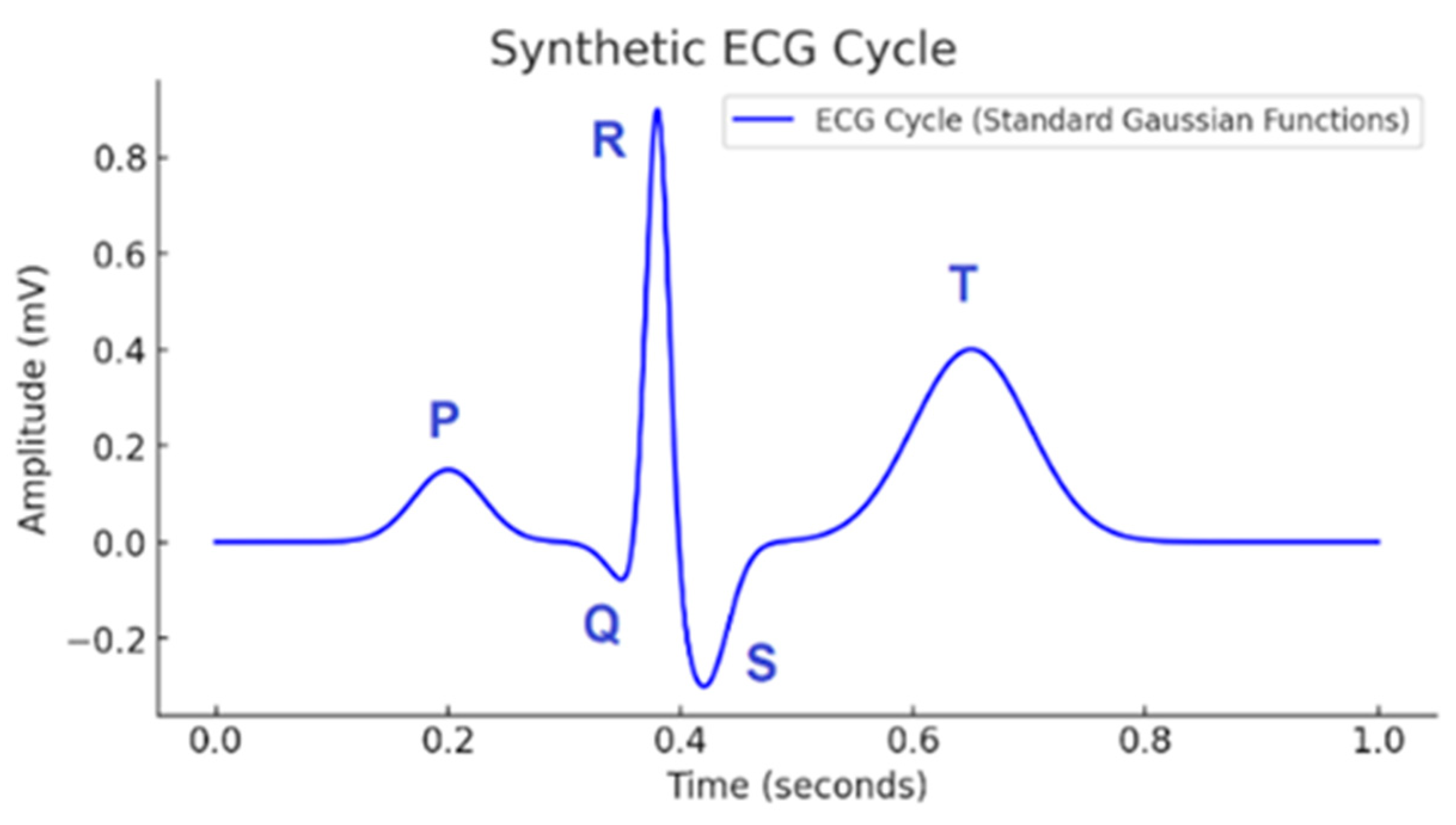
Disclaimer/Publisher’s Note: The statements, opinions and data contained in all publications are solely those of the individual author(s) and contributor(s) and not of MDPI and/or the editor(s). MDPI and/or the editor(s) disclaim responsibility for any injury to people or property resulting from any ideas, methods, instructions or products referred to in the content. |
© 2025 by the author. Licensee MDPI, Basel, Switzerland. This article is an open access article distributed under the terms and conditions of the Creative Commons Attribution (CC BY) license (https://creativecommons.org/licenses/by/4.0/).