Mathematical Formulation of Intensity–Duration–Frequency Curves and Their Hydrological Risk Implications in Civil Engineering Design

Abstract

Intensity–duration–frequency (IDF) curves, which relate rainfall intensity (i), storm duration (d), and return period (T), are cornerstone tools for planning, designing, and operating hydraulic works. Since Sherman’s pioneering formulation in 1931, many modern implementations have systematically omitted the duration-shifting parameter C, causing predicted intensities to diverge to infinity as $d\to 0$. This mathematical paradox becomes especially problematic under extreme hydrological regimes and convective storms exceeding 300 mm/h, where an accurate curve fit is critical. Here, we first review conventional IDF curve fitting techniques and their limitations. We then introduce IDF-GtzLo, a novel, intuitive formulation that reinstates and calibrates C directly from observed storm statistics, ensuring finite intensities for all durations. Applied to 36 automatic weather stations across Mexico, our method reduces the root mean square error by 23 % compared to the classical model. By eliminating the infinite intensity paradox and improving statistical performance, IDF-GtzLo offers a more reliable foundation for hydrological risk assessment and the design of infrastructure resilient to climate-driven extremes.

1. Introduction

IDF curves are mathematical representations of the relationship between the intensity of a storm (i), its duration (d), and the frequency or probability of occurrence (F). This relationship is used to characterize waterworks design events and was first introduced in the 1930s by Sherman (1931) [1]. However, the implementation of these curves gives rise to two issues: one mathematical and the other hydrological.

The first aspect is mathematical. The issue concerns the deduction of IDF curves, as their mathematical development presents a discontinuity. For storm intensities of a short duration (generally for $d\le$ 10 min), the IDF curves theoretically tend towards infinity. This poses a challenge for validating the mathematical expression of the IDF. However, recent extreme hydro-climatological events and unusual records, believed to be caused by climate change, indicate the need for a solution to model the intensities (i) of short-duration storms. Extreme rainfall is often defined as a minimum of $\mathrm{i}\ge$ 70 mm/h [2,3]. However, climate change is currently causing extreme weather events, including hurricanes and heavy rainfall, with intensities greater than $\mathrm{i}\ge$ 300 mm/h. In such circumstances, it is crucial to choose the appropriate IDF curve pattern [4,5].

Despite these known mathematical shortcomings, simplified IDF formulations remain standard in hydraulic works design and review [4]. Large-scale structures, including dam spillways, flood control infrastructure, sewerage projects, roads, and airports, continue to utilize IDF curves in their design.

The second issue is hydrological in nature. The issue pertains to the configuration of the curve. The original formula proposed by Sherman (1931) [1] features a constant (C) that, when added to the storm duration (d)→(C + d), serves as a shape parameter. This means that changes in (C) are directly linked to the shape of the IDF curves. It is important to note that this represents a hydrological problem, as the shape of the curves is directly proportional to the probability of an event occurring. Adding to the controversy, the year after this formula was published, Bernard (1932) [6] proposed the same mathematical expression but without the constant (C), and it was directly widely used. The controversy surrounding the scientific evidence for the calculation of (C) has persisted for over 80 years. To date, the scientific literature has published very little on this subject. To date, only a limited number of scientific papers have suggested a method for estimating (C) [7,8]. Our IDF-GtzLo framework overturns this longstanding simplification by reinstating C as a core calibration parameter. Unlike earlier methods that assign C arbitrarily (or omit it altogether), we derive C directly from observed storm statistics, specifically, the mean short-duration intensity, ensuring finite, physically realistic intensities for all ds.

Although significant progress has been made in understanding extreme events associated with climate change, fundamental questions remain regarding the accurate formulation of intensity–duration–frequency (IDF) curves [9,10]. It is essential to provide solutions that address both the mathematical and hydrological aspects of the problem in a scientific manner. The objective of this research is to use scientific evidence to mathematically deduce the original expression proposed by Sherman (1931) [1] and reduce uncertainty when constructing the IDF curves. A theoretical framework is proposed to demonstrate that a specific value of (C) can accurately fit the probability of extreme event occurrence using IDF curves. This approach is based on the hypothesis that a mathematical formulation, calibrated with high-resolution, short-duration storm data, will resolve the indeterminacy of traditional IDF curves. The expected outcome is that this will produce finite, physically consistent intensities across all durations and improve fit quality compared to existing models.

2. Materials and Methods

2.1. Basic Definitions

In this section, we present a concise characterization of the IDF curves employed in this study and define the fundamental parameters that are their foundation [11].

Definition 1.

Hydrological regime: A regime describes both the magnitude and recurrence of a process over time [2]. Runoff regime: Distribution of flow rates (volume/time). Precipitation regime: Distribution of rainfall depths; Hp normally expressed as intensity $i=Hp/d$ (depth/duration). For a given storm duration d, let Hp denote the observed rainfall depth. The probability of exceeding this depth in any one year is

$$\mathrm{P}(\mathrm{H}\mathrm{p},\mathrm{T})={\displaystyle \frac{1}{\mathrm{T}}}$$

where T is the return period (years). Equivalently, T is defined such that a storm of depth Hp occurs on average once every T years [12]. Intuitive interpretation: IDF curves map the conditional intensity:

$$\mathrm{i}(d,\mathrm{T})={\displaystyle \frac{\mathrm{H}\mathrm{p}}{d}}\to {\mathrm{i}}_d^{\mathrm{T}}={\displaystyle \frac{\mathrm{P}(\mathrm{H}\mathrm{p},\mathrm{T})}{d}}$$

(1)

2.2. Sherman Parameterization

$\mathrm{H}\mathrm{p}={\int }_0^{\mathrm{C}}\mathrm{i} \mathrm{d}\mathrm{t}$. Deriving this expression with respect to C is ${\displaystyle \frac{\partial \mathrm{Hp}}{\partial \mathrm{C}}}=\mathrm{i}\left(\mathrm{C}\right)$; if the total amount of precipitation remains the same as that recorded in the IDF curves, then Hp = Ci. Deriving this expression with respect to C is obtained as follows:

$${\displaystyle \frac{\partial \mathrm{H}\mathrm{p}}{\partial \mathrm{C}}}=\mathrm{i}+\left(\mathrm{C}{\displaystyle \frac{\partial i}{\partial \mathrm{C}}}\right)$$

(2)

The C parameter acts as a “shift” of the duration variable and modulates the overall shape of the curve, so that each ${\left(d-{\mathrm{C}}_{\mathrm{i}}\right)}^{\mathrm{n}\mathrm{i}}$ factor introduces an inflection point or change in slope in the intensity–duration relationship. This means that the value of C adjusts the intensity of precipitation over the duration (d), which can be written as a function of d:

$$\mathrm{F}\left(d\right)={\left(d-{\mathrm{C}}_1\right)}^{{\mathrm{n}}_1}{\left(d-{\mathrm{C}}_2\right)}^{{\mathrm{n}}_2}\cdots {\left(d^2+d+\cdots +{\mathrm{C}}_{\mathrm{i}}\right)}^{{\mathrm{n}}_{\mathrm{i}}}\cdots$$

(3)

For example, a small ${\mathrm{C}}_1$ would capture effects typical of very short storms, while a larger ${\mathrm{C}}_2$ would represent the transition to longer storm regimes. The exponents ${\mathrm{n}}_{\mathrm{i}}$ (not necessarily entire numbers) allow for the modulation of the abruptness or smoothness of the change in slope on the curve.

Substituting in Expression (1), we have

$${\mathrm{i}}_d^{\mathrm{T}}={\displaystyle \frac{\mathrm{k}{\mathrm{T}}^{\mathrm{m}}}{{(d^{\mathsf{\theta }}+\mathrm{C})}^{\mathrm{n}}}}$$

(4)

where i is the rainfall intensity in mm/h. T is the return period ($\mathrm{p}\mathrm{r}\mathrm{o}\mathrm{b}\mathrm{a}\mathrm{b}\mathrm{i}\mathrm{l}\mathrm{i}\mathrm{t}\mathrm{y}={\mathrm{T}}^{-1}$) in years. d is the storm duration in minutes. $\mathrm{k},\mathrm{m},\mathrm{n},\mathrm{C},\mathrm{a}\mathrm{n}\mathrm{d} \mathsf{\theta }$ are parameters that result from any optimization adjustment procedure. The different formulations (4) frequently used in hydrology for the design of hydraulic works are listed in

Table 1. Coefficients of Equation (4) for different authors; adapted [8].

Formulation Known as	Reference	k	m	n	$\mathsf{\theta }$	C
Law of Montana	(Chocat, 1997) [13]	-	-	0	-	-
Sherman	(Sherman, 1931) [1]	-	-	-	1	-
Bernard	(Bernard, 1932) [6]	-	0	1	1	0
Talbot/Linsley 1	(Linsley, et al., 1949) [14]	-	0	1	1	-
Wenzel/Kimijima	(Wenzel, 1982) [15]	-	0	1	-	-
Chow	(Chow, et al., 1988) [16]	-	-	1	1	-
Koutsoyiannis 2	(Koutsoyiannis, et al., 1998) [17]	-	-	-	1	-
Seong	(Seong, 2014) [18]	-	1	$\left(\mathrm{n}·\mathrm{m}\right)$	1	-

¹ Duration (d) between 5 and 20 min and greater than 60 min. ² With ${\mathrm{T}}^{\mathrm{m}}=\mathrm{m}-\mathrm{L}\mathrm{n}[-\mathrm{L}\mathrm{n}\left(1-1/\mathrm{T}\right)].$

.

2.3. Graphic Analysis of IDF Curves

The graphical representation of the IDF curves is straightforward. The abscissa axis represents the storm duration (d), while the ordinate axis represents storm intensity (i). Each curve is associated with a frequency (F) represented by different return periods for the design of hydraulic works (T) [19]. The database, which comprises information from 36 automatic weather stations (AWSs) located in Mexico, utilizes an average of 43 years of recorded data.

Table 2. Historical data example of precipitation intensities in (mm/h) for some duration.

Duration (min)
T (Years)	5	10	20	30	60	120
50	161.3	131.0	106.4	94.2	76.5	62.2
40	141.1	114.6	93.1	82.4	66.9	54.4
30	118.7	96.4	78.3	69.4	56.3	45.8
20	93.1	75.6	61.4	54.4	44.2	35.9
10	61.4	49.9	40.5	35.9	29.1	23.7
5	40.5	32.9	26.7	23.7	19.2	15.6

presents an example of historical records of maximum annual values of intensities for different storm durations at Huimilpan AWS, with records from 2012 to 2024. The return period was calculated using the Weibull formula [20].

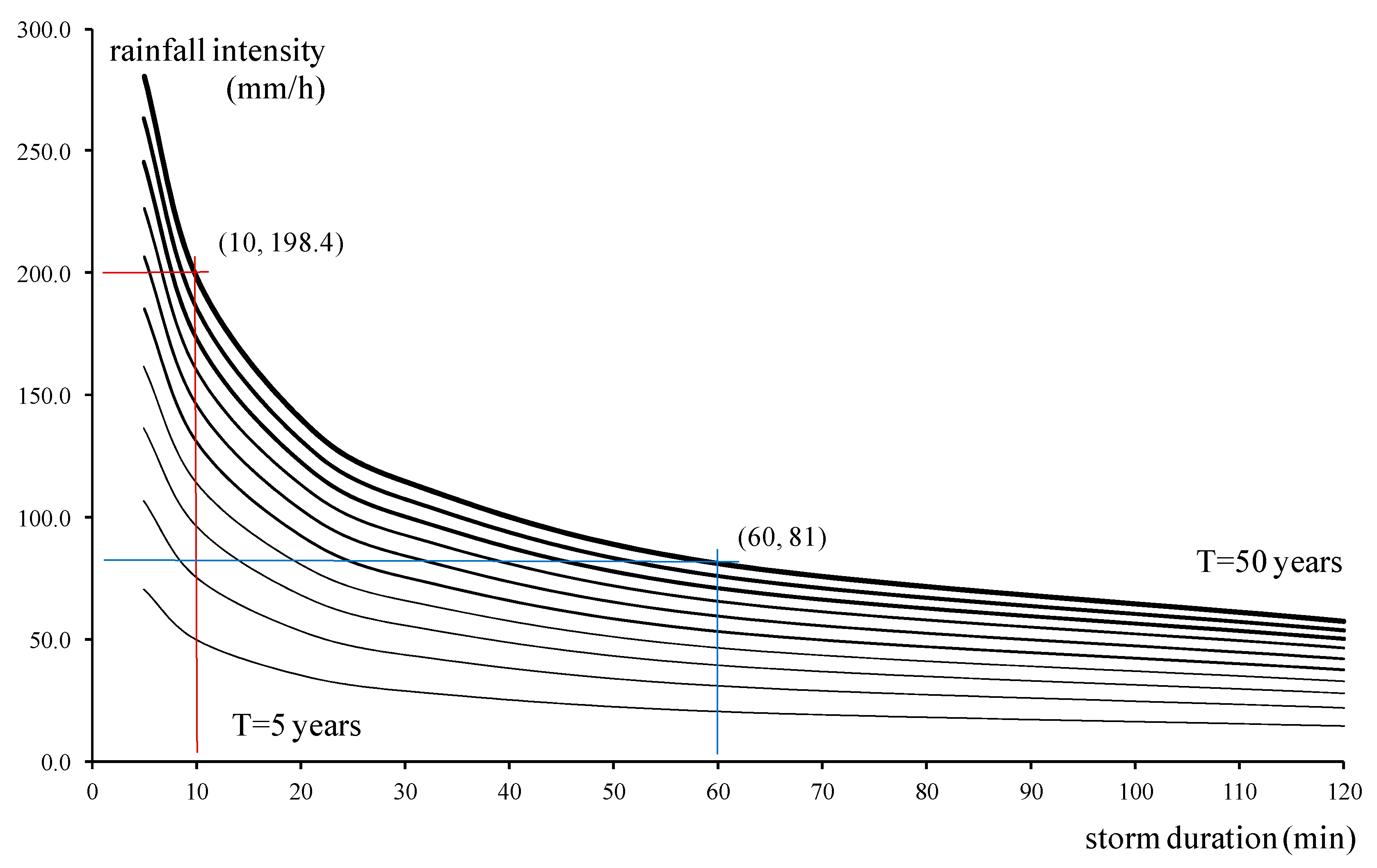
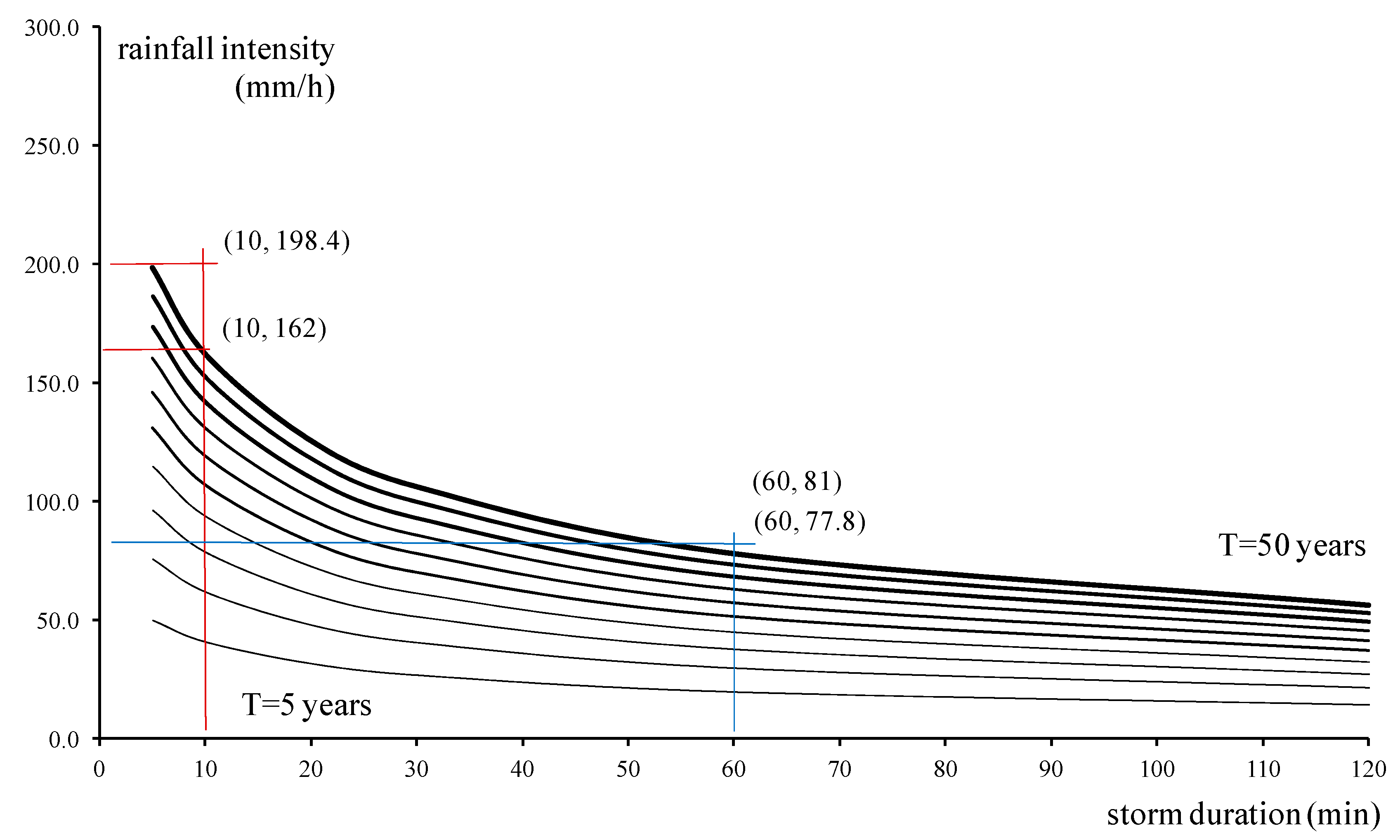
Figure 1 displays the IDF curves calculated for this example based on the equation proposed by Bernard (1932) [6] for a value of C = 0. For durations less than 10 min, Figure 1 shows a significant uncertainty in intensity estimation. This is because the curves tend towards infinity as the duration decreases. The relationship between storm duration (d), storm intensity (i), and frequency (F) was proposed in the 1930s when measurements of precipitation intensities of less than 24 h were scarce. In the contemporary scientific research context, significant progressions have been witnessed in the domains of remote sensing, satellite imagery, and automated weather stations, which have collectively facilitated the monitoring of rainfall at sub-ten-minute intervals. Although hydraulic structures are rarely designed for storms of such brevity, it is crucial to verify that IDF curves remain valid and accurate at these fine temporal scales [21,22]. The problem then lies in the correct positioning of the curves in relation to the measured data. A correct fit without the curves tending to infinity reduces the uncertainty in calculating design events for hydraulic works. This can be demonstrated by examining Figure 1 and Figure 2, which display the same data but with a different value of C. Two points have been selected as examples to demonstrate the behavior of the curves, both for a return period of 50 years. The values of k = 60, n = 0.5, and m = 0.6 are held constant to illustrate the effect of the C parameter. When the parameter is modified, such as changing C to 5 while keeping k, m, and n constant, the curves shift downwards. This effect is frequently overlooked by engineers responsible for hydraulic works.

Table 3. Fitting of the IDF curves for precipitation intensities (mm/h) with C = 0.

Duration (min)
T (Years)	5	10	20	30	60	120
50	280.6	198.4	140.3	114.5	81.0	57.3
45	263.4	186.2	131.7	107.5	76.0	53.8
40	245.4	173.5	122.7	100.2	70.8	50.1
35	226.5	160.2	113.3	92.5	65.4	46.2
30	206.5	146.0	103.3	84.3	59.6	42.2
25	185.1	130.9	92.6	75.6	53.4	37.8
20	161.9	114.5	81.0	66.1	46.7	33.1
15	136.2	96.3	68.1	55.6	39.3	27.8
10	106.8	75.5	53.4	43.6	30.8	21.8
5	70.5	49.8	35.2	28.8	20.3	14.4

and

Table 4. Fitting of IDF curves for precipitation intensities (mm/h) with C = 5.

Duration (min)
T (Years)	5	10	20	30	60	120
50	198.4	162.0	125.5	106.0	77.8	56.1
45	186.2	152.1	117.8	99.6	73.1	52.7
40	173.5	141.7	109.8	92.8	68.1	49.1
35	160.2	130.8	101.3	85.6	62.8	45.3
30	146.0	119.2	92.4	78.1	57.3	41.3
25	130.9	106.9	82.8	70.0	51.3	37.0
20	114.5	93.5	72.4	61.2	44.9	32.4
15	96.3	78.7	60.9	51.5	37.8	27.2
10	75.5	61.7	47.8	40.4	29.6	21.4
5	49.8	40.7	31.5	26.6	19.5	14.1

present the IDF curves in Figure 1 and Figure 2 with numerical values.

As demonstrated in Figure 1 (corresponding to C = 0), the IDF curves for T = 50 years exhibit a pronounced asymptotic growth when the duration d tends to zero. For instance, at d = 10 min, the estimated intensity is 198.4 mm/h, and for d = 5 min (red line), it exceeds 280 mm/h. This configuration is indicative of the “infinite paradigm” inherent within the classical formulation. As demonstrated in Figure 2, when displacement C is incorporated, the curves “flatten” within the short duration range (d = 10 min): the intensity diminishes to 162 mm/h (red line), and for d = 60 min, the value fluctuates between 81 mm/h and 77.8 mm/h (blue line).

2.4. Understanding the Role of Parameter C

Now that it has been demonstrated that parameter C has a direct relationship with the shape of the curves, it is necessary to verify this mathematically [21,23]. Therefore, it is proposed to establish the limit of the initial formulation.

Lemma 1

(Finiteness). Taking the limit of (Equation (4)), it is obtained that i(d,T) is finite for all d ≥ 0 if and only if C > 0.

$$\underset{d\to 0}{\lim }{\displaystyle \frac{\mathrm{k}{\mathrm{T}}^{\mathrm{m}}}{{\left(d+\mathrm{C}\right)}^{\mathrm{n}}}}={\displaystyle \frac{\mathrm{k}{\mathrm{T}}^{\mathrm{m}}}{{\mathrm{C}}^{\mathrm{n}}}}<\infty \iff C>0$$

$$\underset{d\to 0}{\lim }{\displaystyle \frac{\mathrm{k}{\mathrm{T}}^{\mathrm{m}}}{{\left(d+\mathrm{C}\right)}^{\mathrm{n}}}}={\displaystyle \frac{\underset{d\to 0}{\lim }\mathrm{k}{\mathrm{T}}^{\mathrm{m}}}{\underset{d\to 0}{\lim }{\left(d+\mathrm{C}\right)}^{\mathrm{n}}}}={\displaystyle \frac{\mathrm{k}{\mathrm{T}}^{\mathrm{m}}}{\underset{d\to 0}{\lim }\left[\left(\begin{array}{c}\mathrm{n}\\ 0\end{array}\right)d^{\mathrm{n}}{\mathrm{C}}^0+\left(\begin{array}{c}\mathrm{n}\\ 1\end{array}\right)d^{\mathrm{n}-1}\mathrm{C}+\cdots +\left(\begin{array}{c}\mathrm{n}\\ \mathrm{n}\end{array}\right){\mathrm{C}}^{\mathrm{n}}\right]}}={\displaystyle \frac{\mathrm{k}{\mathrm{T}}^{\mathrm{m}}}{{\mathrm{C}}^{\mathrm{n}}}}$$

In this expression, k sets the vertical scale of intensity (how high the curves are, on average); m controls how much the intensity increases when moving to rarer events (longer return period T); n governs how quickly the intensity decreases as the duration d increases; and C acts as a time shift representing a minimum effective duration, preventing the intensity from becoming infinite when d tends to zero. This is the essence of Lemmas 1: given a positive constant C, the intensity remains finite for any duration, a property that aligns with real physical processes and measurement resolutions.

Corollary 1.

The function i(d,T) is continuous and infinitely differentiable on [0,∞).

For real values of the storm intensity (i), this result indicates C could be different from zero. However, this condition is often disregarded in most applications of IDF curves, with many researchers choosing to eliminate C without providing any explanation.

Lemma 2.

Use this result to obtain real values of precipitation intensity in (mm/h). The obtained limit can be delimited if

$${\displaystyle \frac{\mathrm{k}{\mathrm{T}}^{\mathrm{m}}}{{\mathrm{C}}^{\mathrm{n}}}}\le {\mathrm{i}}_{\mathrm{r}\mathrm{e}\mathrm{a}\mathrm{l}}\to {\left({\displaystyle \frac{\mathrm{k}{\mathrm{T}}^{\mathrm{m}}}{{\mathrm{i}}_{\mathrm{r}\mathrm{e}\mathrm{a}\mathrm{l}}}}\right)}^{{\displaystyle \raisebox{1ex}{$1$}\!\left/ \!\raisebox{-1ex}{$\mathrm{n}$}\right.}}\le \mathrm{C}$$

(5)

Given an observed intensity ${\mathrm{i}}_{\mathrm{r}\mathrm{e}\mathrm{a}\mathrm{l}}$ at a specific duration d and return period T, the shape parameter C must satisfy

$${\displaystyle \frac{\mathrm{k}{\mathrm{T}}^{\mathrm{m}}}{{\left(d_0+C\right)}^{\mathrm{n}}}}\le {\mathrm{i}}_{\mathrm{r}\mathrm{e}\mathrm{a}\mathrm{l}}\to \mathrm{C}\ge {\left({\displaystyle \frac{\mathrm{k}{\mathrm{T}}^{\mathrm{m}}}{{\mathrm{i}}_{\mathrm{r}\mathrm{e}\mathrm{a}\mathrm{l}}}}\right)}^{{\displaystyle \raisebox{1ex}{$1$}\!\left/ \!\raisebox{-1ex}{$\mathrm{n}$}\right.}}-d_0$$

This inequality provides a direct, empirical route to estimate a lower bound for C from field measurements $\left(d_0,{\mathrm{i}}_{\mathrm{r}\mathrm{e}\mathrm{a}\mathrm{l}} \right)$. By inverting the IDF formula at any observed storm intensity, one obtains a data-driven value of C that ensures finite, physically realistic predictions.

This means that the value of C is dependent on the return period (in years) and the corresponding rainfall intensity (mm/h). This finding is consistent with the results obtained by Gutierrez et al. (2019) [8], who suggested that C represents a function of the mean storm duration in the study area, which is equivalent to T = 2.33 years in probabilistic terms [24,25].

2.5. Sensitivity and Convexity Analysis

Compute derivatives to assess parameter sensitivity and convexity with respect to d.

Lemma 3

(Parameter Estimation). For an observed intensity $i_{obs}$ at duration $d_0$ and return period T, the shape parameter satisfies

$$\mathrm{C}={\left({\displaystyle \frac{\mathrm{k}{\mathrm{T}}^{\mathrm{m}}}{{\mathrm{i}}_{\mathrm{o}\mathrm{b}\mathrm{s}\left(\mathrm{r}\mathrm{e}\mathrm{a}\mathrm{l}\right)}}}\right)}^{{\displaystyle \raisebox{1ex}{$1$}\!\left/ \!\raisebox{-1ex}{$\mathrm{n}$}\right.}}-d_0$$

Lemma 4

(Derivative and Sensitivity). The partial derivatives are

$${\displaystyle \frac{\partial \mathrm{i}}{\partial d}}-{\displaystyle \frac{\mathrm{k}{\mathrm{T}}^{\mathrm{m}}}{{\left(d+\mathrm{C}\right)}^{\mathrm{n}}}}, {\displaystyle \frac{\partial \mathrm{i}}{\partial \mathrm{k}}}={\displaystyle \frac{{\mathrm{T}}^{\mathrm{m}}}{{\left(d+\mathrm{C}\right)}^{\mathrm{n}}}}, {\displaystyle \frac{\partial \mathrm{i}}{\partial \mathrm{m}}}={\displaystyle \frac{\mathrm{k}{\mathrm{T}}^{\mathrm{m}}\ln \mathrm{T}}{{\left(d+\mathrm{C}\right)}^{\mathrm{n}}}}$$

$${\displaystyle \frac{\partial \mathrm{i}}{\partial \mathrm{n}}}=-\mathrm{i}\left(d,\mathrm{T}\right)\mathrm{Ln}\left(d+\mathrm{C}\right), {\displaystyle \frac{\partial \mathrm{i}}{\partial \mathrm{C}}}=-\mathrm{n}{\displaystyle \frac{\mathrm{k}{\mathrm{T}}^{\mathrm{m}}}{{\left(d+\mathrm{C}\right)}^{\mathrm{n}+1}}}$$

Then the Asymptotic Behavior could be noted as

$$\underset{d\to \mathrm{\infty }}{\lim }\mathrm{i}\left(d,\mathrm{T}\right)~\mathrm{k}{\mathrm{T}}^{\mathrm{m}}{d}^{-\mathrm{n}}, \underset{d\to 0}{\lim }\mathrm{i}\left(d,\mathrm{T}\right)={\displaystyle \frac{\mathrm{k}{\mathrm{T}}^{\mathrm{m}}}{{\mathrm{C}}^{\mathrm{n}}}}$$

Convergence on

$(d_0,\mathrm{\infty })$ with $d_0>0$ follows from the continuous differentiability of $\mathrm{i}\left(d,\mathrm{T}\right)$.

Lemma 4 translates the intuition of the first one into a sensitivity. Increases in k or m result in elevated intensity levels, as demonstrated by the given ${\displaystyle \frac{\partial \mathrm{i}}{\partial \mathrm{k}}}>0, {\displaystyle \frac{\partial \mathrm{i}}{\partial \mathrm{m}}}=\mathrm{i} \mathrm{L}\mathrm{n}\mathrm{T}>0$. Conversely, elevations in n, C, or d lead to a reduction in intensity levels, as indicated by ${\displaystyle \frac{\partial \mathrm{i}}{\partial \mathrm{n}}}=-\mathrm{i}\mathrm{Ln}\left(d+\mathrm{C}\right)<0,{\displaystyle \frac{\partial \mathrm{i}}{\partial \mathrm{C}}}=-\mathrm{n}{\displaystyle \frac{\mathrm{k}{\mathrm{T}}^{\mathrm{m}}}{{\left(d+\mathrm{C}\right)}^{\mathrm{n}+1}}}<0, {\displaystyle \frac{\partial \mathrm{i}}{\partial \mathrm{d}}}={\displaystyle \frac{\partial \mathrm{i}}{\partial \mathrm{C}}}$. From a physical perspective, this signifies that the frequency of the event (via m) and the regional scale of rainfall (via k) result in an upward shift in the curve. Temporal smoothing (via n) and the effective mean duration (via C) serve to moderate the curve, particularly in short durations where the effect is most intense [8]. Therefore, the parameters delineate distinct roles: k and m contribute “how much” and “how rare” the event is, respectively; n and C govern “how” that intensity is distributed over time. This reading facilitates the interpretation of design changes. For instance, an increase in m primarily affects events with a long T, while adjustments in C and n have a critical impact on the short duration section. In this context, the parameter k exhibits a direct proportionality to precipitation intensities.

3. The New Alternative Curves IDF-GtzLo

The present study proposes an innovative framework for curve construction, namely IDF-GtzLo, with the aim of overcoming the limitations of existing intensity–duration–frequency (IDF) models. The infinite intensity paradox at short durations and the ad hoc treatment of the duration-shift parameter C are two such limitations. The reintroduction of C as an empirically calibrated parameter serves to enforce finite intensities across all durations, thereby facilitating a more faithful capture of storm behavior. In contrast to earlier methods that either omit or arbitrarily assign C, IDF-GtzLo derives C directly from observed short-duration storm statistics. In the subsequent sections, the mathematical derivation, calibration procedure, and performance evaluation of IDF-GtzLo across diverse climatic stations are described.

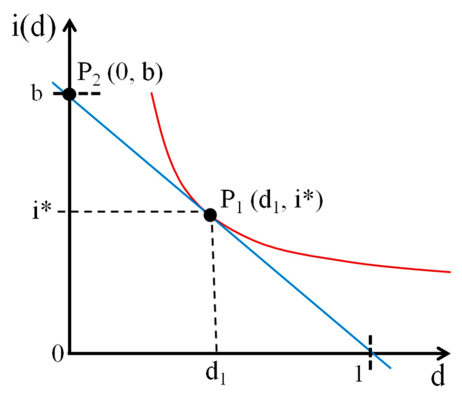
In Figure 3, point ${\mathrm{P}}_1$ on the curve (red line) for a certain T has the coordinates $\left(d_1,{\mathrm{i}}^{\ast }\right)$. If the derivative at that point is calculated, it can be obtained as follows:

$${\displaystyle \frac{\partial \left({\mathrm{d}}_1\right)}{\partial d}}={\displaystyle \frac{\partial }{\partial d}}\left[{\displaystyle \frac{\mathrm{k}{\mathrm{T}}^{\mathrm{m}}}{{\left(d+\mathrm{C}\right)}^{\mathrm{n}}}}\right]=\mathrm{k}{\mathrm{T}}^{\mathrm{m}}\left(-\mathrm{n}\right){(d+\mathrm{C})}^{-(\mathrm{n}+1)}=\mathrm{m}$$

(6)

The slope of the line through point ${\mathrm{P}}_1$ is represented by the calculated m (blue line). Additionally, the line through ${\mathrm{P}}_1$ can be operated to determine the ordinate to the origin.

$${\mathrm{i}}^{\ast }=\mathrm{m}·d_1+\mathrm{b};\mathrm{b}={\mathrm{i}}^{\ast }-\mathrm{m}·d_1$$

Substituting (4), it follows that

$${\displaystyle \frac{\mathrm{k}{\mathrm{T}}^{\mathrm{m}}}{{\left(d+\mathrm{C}\right)}^{\mathrm{n}}}}-\mathrm{k}{\mathrm{T}}^{\mathrm{m}}\left(-\mathrm{n}\right){(d+\mathrm{C})}^{-(\mathrm{n}+1)}=\mathrm{b}$$

Rearranging and considering that the derivative is taken at ${\mathrm{P}}_1$, it is obtained as follows:

$${\displaystyle \frac{\mathrm{k}{\mathrm{T}}^{\mathrm{m}}}{{\left(d_1+\mathrm{C}\right)}^{\mathrm{n}}}}+{\displaystyle \frac{\mathrm{k}{\mathrm{T}}^{\mathrm{m}}\left(\mathrm{n}\right)d_1}{{(d_1+\mathrm{C})}^{(\mathrm{n}+1)}}}=\mathrm{b}$$

By factoring

$${\mathrm{i}}^{\ast }=\mathrm{b}=\mathrm{k}{\mathrm{T}}^{\mathrm{m}}\left[{\displaystyle \frac{1}{{\left(d_1+\mathrm{C}\right)}^{\mathrm{n}}}}+{\displaystyle \frac{\mathrm{n}·d_1}{{(d_1+\mathrm{C})}^{(\mathrm{n}+1)}}}\right] \mathrm{w}\mathrm{i}\mathrm{t}\mathrm{h} \mathrm{C}\ne 0$$

(7)

$${\mathrm{i}}^{\ast }=\mathrm{b}=\mathrm{k}{\mathrm{T}}^{\mathrm{m}}\left[{\displaystyle \frac{1}{{\left(d_1\right)}^{\mathrm{n}}}}+{\displaystyle \frac{\mathrm{n}·d_1}{{\left(d_1\right)}^{(\mathrm{n}+1)}}}\right] \mathrm{w}\mathrm{i}\mathrm{t}\mathrm{h} \mathrm{C}=0$$

(8)

The proposed formulation, which is now ninety years old, aims to eliminate uncertainty in the shape and position of the IDF curves. The parameters k, m, n, and C are to be obtained from the measured historical data record.

4. Results

We analyzed the maximum annual intensities from 36 AWSs across Mexico for durations $d=5, 10, 20, 30, 60, \mathrm{a}\mathrm{n}\mathrm{d} 120$ min and return periods $\mathrm{T}=5, 10, 25, \mathrm{a}\mathrm{n}\mathrm{d} 50$ years. Parameters k, m, n, and C were fitted via nonlinear least squares minimizing the RMSE and Nash–Sutcliffe efficiency (NSE).

Application of the Proposed Example

Referring to Table 2 and Figure 1 and Figure 2, it is evident that there is a point on the duration axis where the value of C is no longer critical. To locate the value of intensities for the same storm duration, such as 60 min, use $i=81 \mathrm{m}\mathrm{m}/\mathrm{h} \mathrm{f}\mathrm{o}\mathrm{r} \mathrm{C}=0 \mathrm{a}\mathrm{n}\mathrm{d} i=77.8 \mathrm{m}\mathrm{m}/\mathrm{h} \mathrm{f}\mathrm{o}\mathrm{r} \mathrm{C}=5$. The difference in intensities is only $∆i=3.2 \mathrm{m}\mathrm{m}/\mathrm{h}$. This is consistent with Bernard’s (1932) [6] omission of this parameter. However, the position of the curves for short durations, such as 10 min, presents an extreme behavior that tends towards infinity. To locate the value of the intensities for a storm duration of 10 min, use the following values: $\mathrm{i}=198.4 \mathrm{m}\mathrm{m}/\mathrm{h} \mathrm{f}\mathrm{o}\mathrm{r} \mathrm{C}=0 \mathrm{a}\mathrm{n}\mathrm{d} \mathrm{i}=162 \mathrm{m}\mathrm{m}/\mathrm{h} \mathrm{f}\mathrm{o}\mathrm{r} \mathrm{C}=5$. The difference in intensities is $∆i=36.4 \mathrm{m}\mathrm{m}/\mathrm{h}$. This value, if transformed into hydrological risk, may result in the imprecise calculation of the design event.

In relation to hydrological risk, failure risk due to a hydrological extreme event is defined as the probability of exceedance in N consecutive years if an event return period T occurs. It can also be used to calculate the probability of a hydrological event occurring during a period of N years [26,27]. The failure risk can be expressed as a function of the return period and can be calculated as follows:

$$\mathrm{R}=1-{\left[1-\mathrm{P}\left(\mathrm{x}\right)\right]}^{\mathrm{N}}\to \mathrm{R}=1-{\left(1-{\displaystyle \frac{1}{\mathrm{T}}}\right)}^{\mathrm{N}}$$

(9)

where

R is the risk of failure within the useful life of the hydraulic civil work or the probability of occurrence of a hydrological event.

N is the number of years of the useful life of the hydraulic civil work or the occurrence period of a hydrological event.

For example, when designing a structure with a lifetime of N = 50 years, a storm duration of 30 min and a proposed design event of 100 mm/h, using the traditional formulation of the IDF curves, result in an increase in risk of over 18% due to the change in the return period. However, by setting the curves on the intensity axis, as proposed, the risk would only increase by 4%.

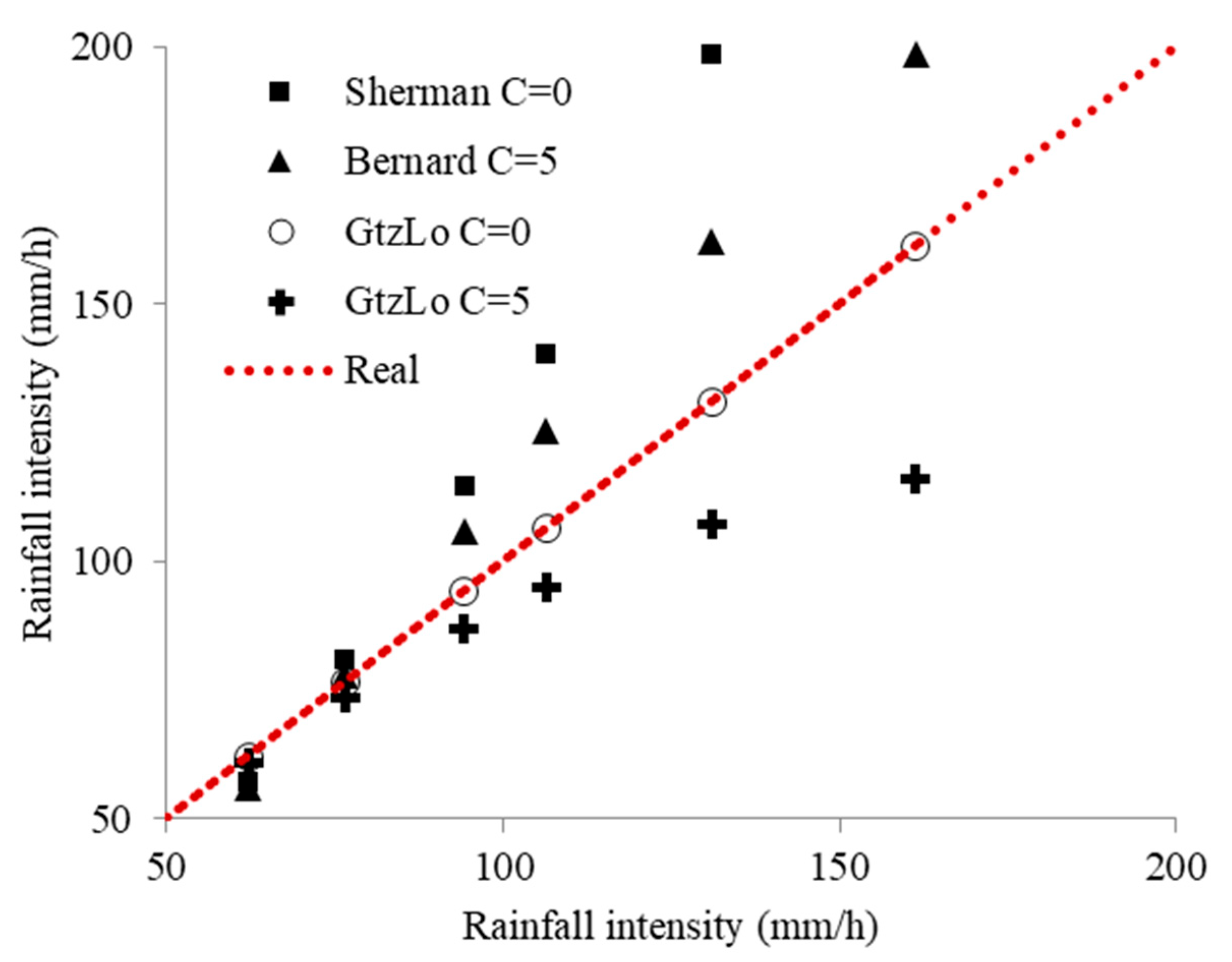
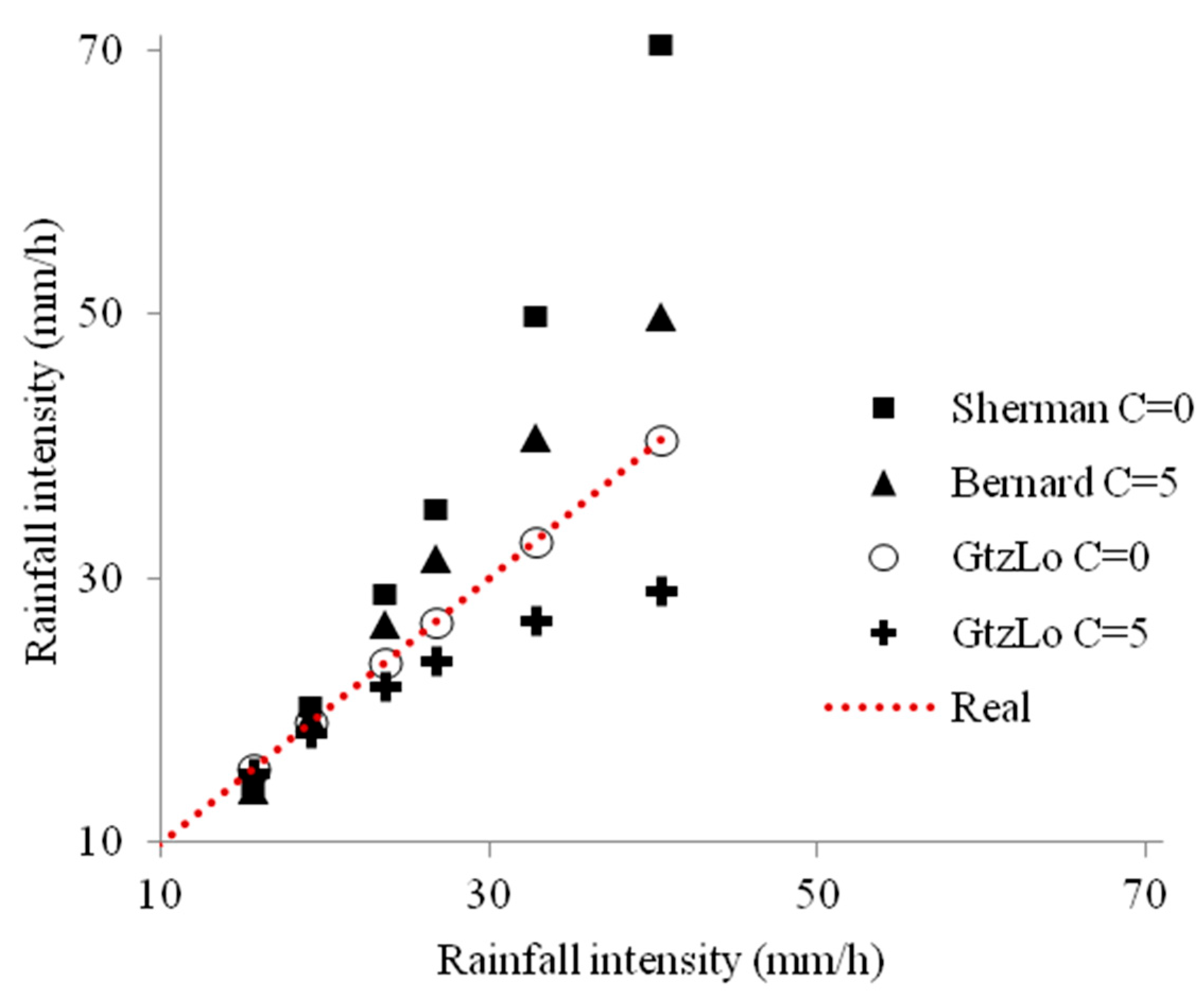
Figure 4 and Figure 5 compare the values obtained using the different formulations proposed in this paper for the example. The results show a difference between using curves that tend to infinity and curves that are stable with a mathematically calculated intensity value for the smallest measured storm duration. This new formulation eliminates the need to fit any theoretical probability distribution to the values of the recorded intensities. It is understood that once the curves are fully defined and located without any mathematical indefinition, the design events are obtained with parallel IDF curves. In practice, the calibration of (k, m, n, and C) is derived directly from observed intensities and plotting-position frequencies, without imposing a GEV-Gumbel family. Once these parameters have been established for a given site, the design intensities for any (d, T) are subsequently determined through direct substitution. Updates to these parameters are facilitated by re-estimating (k, m, n, C) as new data becomes available.

Including C prevents divergence for $d<10 \mathrm{m}\mathrm{i}\mathrm{n}$, yielding finite intensities consistent with the observed maxima (e.g., at T = 50 yr, d = 5 min: ${\mathrm{i}}_{\mathrm{C}=0}\approx 280.6 \mathrm{m}\mathrm{m}/\mathrm{h} \mathrm{v}\mathrm{s}. {\mathrm{i}}_{\mathrm{C}=5}\approx 198.4 \mathrm{m}\mathrm{m}/\mathrm{h}$; RMSE decreased by 23% and NSE increased from 0.82 to 0.94 when fitting IDF-GtzLo vs. classical model. Hydrological risk for T = 25 yr, N = 50 yr: Classical: $\mathrm{R}\approx 86\mathrm{\%}$; IDF-GtzLo: $\mathrm{R}\approx 70\mathrm{\%}$).

5. Discussion

Discussion of the New Formulation IDF-GtzLo in Mexico

Traditionally in Mexico, the IDF curves are derived from studies conducted by the Ministry of Communications and Transport (SCT). It is noteworthy that the National Water Commission, rather than the SCT, should be responsible for calculating and publishing these curves. However, for years, the IDF-SCT curves have been the reference in the design of civil hydraulic works.

In Mexico, the Comision de Caminos y Puentes Federales (SCT) publishes standardized IDF curves that are widely used for hydraulic design. Their procedure typically (1) adopts Sherman’s original functional form with the duration-shift parameter fixed at C = 0, (2) pools multi-year rainfall records across broad regions, and (3) fits only two coefficients (intensity scale k and decay exponent n via linear regression on log–log transformed data). By holding C at zero, SCT curves inherently allow intensities to diverge for short durations and cannot adapt to local storm microstructure. In contrast, IDF-GtzLo reintroduces C as a third calibration parameter derived directly from site-specific, short-duration observations and uses the nonlinear optimization of all three parameters (k,m,n,C). As a result, IDF-GtzLo produces finite, physically plausible intensities at d ≤ 10 min and significantly reduces fitting errors compared to the SCT approach.

The purpose of this paper is not to provide a detailed development showing the differences between the IDF-SCT and IDF-GtzLo curves for all automatic weather stations in Mexico. Such a comparison would require calculating intensities for a variety of combinations across the entire territory. However, it is important to provide a simple comparison of the potential results and implications of using the findings of this research.

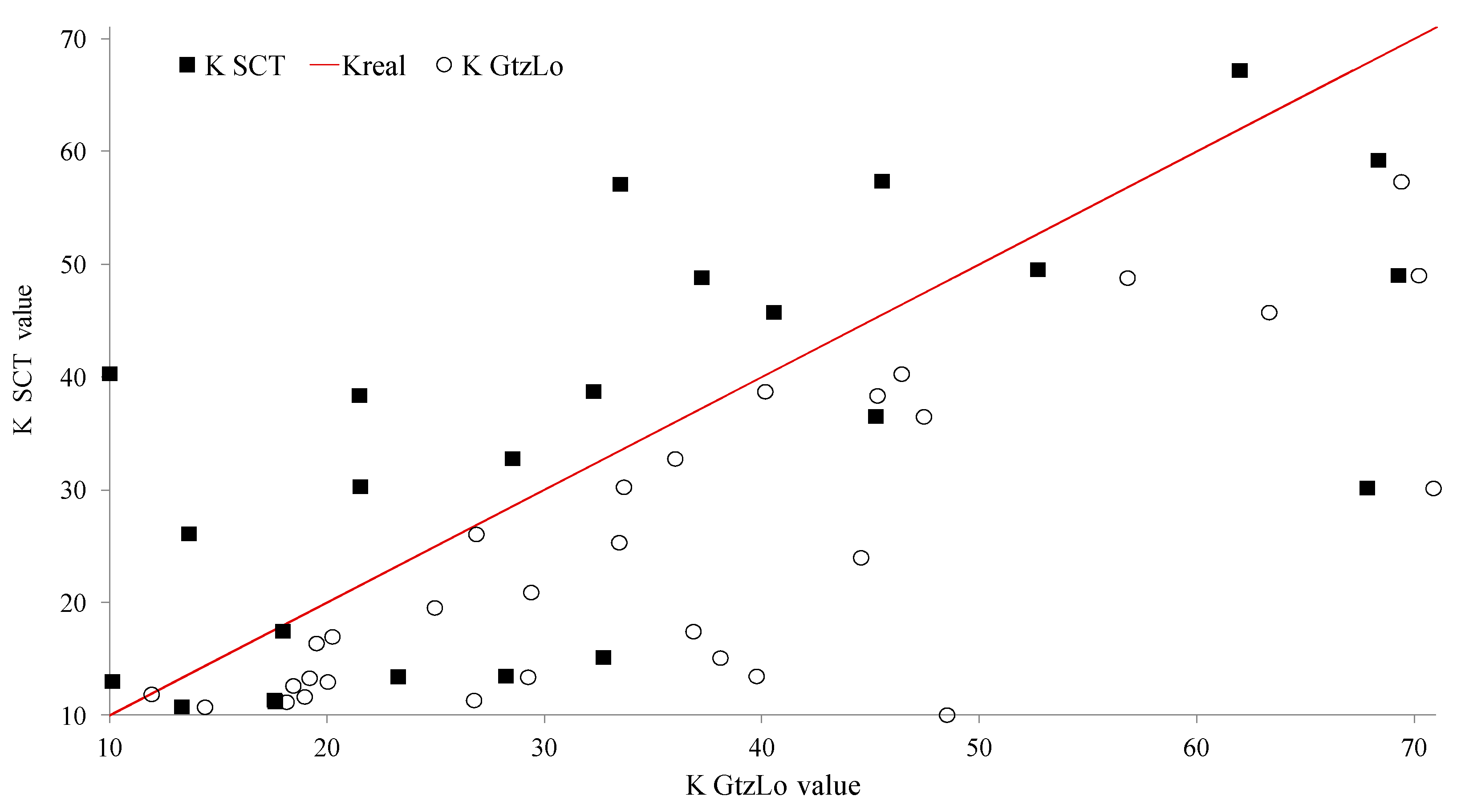
Therefore, the suitability of both IDF-SCT and IDF-GtzLo formulations was compared by examining the parameter k, which is directly proportional to the return period and precipitation intensity. Figure 6 illustrates the results for the 36 primary automatic weather stations (AWSs) in Mexico. Additionally, Appendix A provides the IDF-GtzLo curve parameters for these stations, which can be immediately applied and used. It should be noted that the widespread adoption of this new formulation would require a review of works, structures, projects, and necessary infrastructure to consistently improve the safety of people and their property in relation to hydraulic design.

The formal reinstatement of C resolves the mathematical inconsistency and aligns model outputs with physical rainfall processes. A sensitivity analysis (Equation (4)) shows C and n as dominant parameters for short-duration event predictions. Results recommend updating national IDF standards (e.g., SCT) to incorporate continuous parameter calibration.

As illustrated in

Table 5. Performance measures and goodness of fit of the proposed formulations.

Fit/Error Method	IDF-SCT	IDF-GtzLo
(Mean Absolute Error) $\mathrm{M}\mathrm{A}\mathrm{E}={\displaystyle \frac{1}{\mathrm{N}}}{\displaystyle {\sum }_{\mathrm{i}=1}^{\mathrm{N}}}\left|{\mathrm{k}}_{\mathrm{i}}-{\widehat{\mathrm{k}}}_{\mathrm{i}}\right|$	13.45	16.45
(Root Mean Square Error) $\mathrm{R}\mathrm{M}\mathrm{S}\mathrm{E}=\sqrt{{\displaystyle \frac{1}{\mathrm{N}}}{\displaystyle {\sum }_{\mathrm{i}=1}^{\mathrm{N}}}\left|{\mathrm{k}}_{\mathrm{i}}-{\widehat{\mathrm{k}}}_{\mathrm{i}}\right|}$	21.49	24.65
(Mean Absolute Percentage Error) $\mathrm{M}\mathrm{A}\mathrm{P}\mathrm{E}={\displaystyle \frac{100\mathrm{\%}}{\mathrm{N}}}{\displaystyle {\sum }_{\mathrm{i}=1}^{\mathrm{N}}}\left|{\displaystyle \frac{{\mathrm{k}}_{\mathrm{i}}-{\widehat{\mathrm{k}}}_{\mathrm{i}}}{{\mathrm{k}}_{\mathrm{i}}}}\right|$	207.205	353.88
(Median Absolute Error) $\mathrm{M}\mathrm{e}\mathrm{d}\mathrm{A}\mathrm{E}=\mathrm{m}\mathrm{e}\mathrm{d}\mathrm{i}\mathrm{a}\mathrm{n}\left(\left|{\mathrm{k}}_{\mathrm{i}}-{\widehat{\mathrm{k}}}_{\mathrm{i}}\right|\right)$	8.477	10.032
(Pearson) $\mathrm{R}=\mathrm{C}\mathrm{o}\mathrm{v}\left({\mathrm{k}}_{\mathrm{i}},{\widehat{\mathrm{k}}}_{\mathrm{i}}\right)/\sqrt{\mathrm{V}\mathrm{a}\mathrm{r}\left({\mathrm{k}}_{\mathrm{i}}\left)\mathrm{V}\mathrm{a}\mathrm{r}\right({\widehat{\mathrm{k}}}_{\mathrm{i}}\right)}$	0.649	0.855
R2	0.422	0.730
(Error Variances) ${\mathrm{e}}_{\mathrm{i}}={\widehat{\mathrm{k}}}_{\mathrm{i}}-{\mathrm{k}}_{\mathrm{i}}$; $\mathrm{V}\mathrm{a}\mathrm{r}(\mathrm{e})={\displaystyle \frac{1}{\mathrm{N}}}{\displaystyle {\sum }_{\mathrm{i}=1}^{\mathrm{N}}}{\left({\mathrm{e}}_{\mathrm{i}}-\overline{\mathrm{e}}\right)}^2$	466.004	342.509

, the goodness-of-fit test values for the k values calculated by IDF-SCT and IDF-GtzLo are presented. The SCT method demonstrated a lower mean absolute error (MAE) and root mean square error (RMSE) in comparison to IDF-GtzLo, indicating a more precise alignment with the observed k values. However, it should be noted that these results may vary depending on the selection of stations and the quality of the data. With regard to the issue of correlation, the IDF-GtzLo method demonstrated a correlation of 0.85 with the observed data in comparison to the 0.65 correlation achieved by the SCT method. Should the explained variance be utilized as an indicator, the coefficient of determination R2 of GtzLo (0.73) would indicate that it explains 73% of the variability of k in comparison to only 42% for SCT. This analysis reveals that, although the mean absolute error of SCT may be lower in some cases, the IDF-GtzLo models the overall trend of the data significantly more accurately, better capturing the structure of variation in k between stations.

A closer analysis reveals that the variance of the absolute errors of GtzLo is considerably lower than that of SCT, suggesting that while SCT may exhibit a lower mean absolute error (MAE) in certain instances, the errors of GtzLo are more concentrated around zero. This finding suggests a heightened degree of stability and reliability in the predictions made by the proposed methodology. The greater correlation with the observed data and the lower variance of the errors make IDF-GtzLo the most robust option for estimating the k parameter. The findings of this study serve to reinforce the notion that the calibration of the C parameter through empirical means, in conjunction with the utilization of nonlinear optimization techniques, represents a superior approach when compared with traditional SCT methodologies.

The parameter k functions as a scaling factor for intensity in Sherman’s formula (Equation (4)). It is evident that an elevated k results in a shift in the curve towards higher intensities across the entire range of durations. This has resulted in a shift towards more conservative designs, as the sizing of structures will need to account for increased levels of precipitation that exceed the historical record. A lower k results in lower estimated intensities, which can lead to an underestimation of extreme events and, consequently, to potentially undersized infrastructure.

The propagation error of the new formulation should be reviewed once it is applied to a whole region and to an exhaustive sample of data with extremes. However, it is not the subject of this paper, but it is suggested that the propagation error should be estimated by the Delta Method, for example. As demonstrated in Appendix B, the application of the Delta Method is illustrated in the design of a hydraulic structure.

While the findings are based on 36 automatic stations in Mexico, with mean records over 40 years, the database is extensive and climatically diverse (convection, orographic effects, and tropical cyclones). The evaluations are contrasted with the actual design values used in national practice. The central contribution of this study is a crucial rectification of a long-standing mathematical inconsistency in the IDF formulation. This rectification is achieved while preserving continuity with engineering practice. It is acknowledged that the universality of the model still needs to be verified outside of Mexico. Future research will expand validation in contrasting climate zones worldwide, evaluating the transferability of (k, m, n, and C) and the need for regional recalibration.

6. Conclusions

The aim of this study is to propose an alternative mathematical formulation for the traditional IDF curves. It is apparent that IDF curves are often used without considering the implications of their shape and position on the design of hydraulic works. This is particularly relevant given that extreme phenomena, such as torrential rainfall, can now be monitored in real-time or in very small time lapses. The research findings suggest that the C parameter should be used or revised based on short-term measurements. One significant finding of this study is the potential to “fix” the curves at the ordinate axis (representing precipitation intensities) from tending towards infinity. This approach reduces uncertainty in estimating design events. It has been suggested that Sherman’s (1931) model [1] is a limited model in conditions of extreme short-term rainfall, and its mathematical clarity can be enhanced with the proposed expressions. Furthermore, this study offers an explanation for the utilization of the new IDF curve proposal, as the added terms are the same parameters that are traditionally calculated. It may be worthwhile for future studies in this field to explore the inclusion of other factors, such as geographic position and the useful life of hydraulic works. In the context of geographical location, ongoing studies building upon the methodological framework outlined herein have identified a correlation between the geographical attributes of the stations, including latitude and distance from the ocean, and the value of the k parameter. Furthermore, the hydrological risk estimated with multiple probability distributions can be associated with regional values of the useful life of hydraulic works (See Equation (9)).

We provide a rigorous mathematical framework for IDF curves, demonstrating that the shape parameter C is both necessary for finiteness and influential in risk estimation. The IDF-GtzLo formulation offers an improved fit, reduced uncertainty, and actionable insights for infrastructure design under extreme rainfall.

Finally, beyond resolving the mathematical divergence at short durations, the reintroduction and empirical calibration of C offer quantifiable improvements in performance. In 36 automatic stations in Mexico, the IDF-GtzLo reduced the root mean square error (RMSE) by approximately 23% and increased the Nash–Sutcliffe efficiency from 0.82 to 0.94. Additionally, for the scale factor k, it explained 73% of the observed variability (R² = 0.73) compared to 42% for the SCT approach and decreased the variance of errors by ~27%. In an example of urban drainage sizing (10 min, 50 years), IDF-GtzLo intensities implied 18% lower flows, 9.6% smaller diameters, and savings of 361 USD/m, while maintaining physical consistency in the short duration range. While the findings are contingent on the specific location and the data resolution, they demonstrate that the benefit is both operational and conceptual. Subsequent research endeavors will incorporate uncertainty propagation (Delta Method) and regional validations to support the updating of IDF standards.

References

1. Sherman, C.W. Frequency and Intensity of Excessive Rainfalls at Boston, Massachusetts. Trans. Am. Soc. Civ. Eng. 1931, 95, 951–960. [Google Scholar] [CrossRef]
2. Gutierrez-Lopez, A. Methodological Guide to Forensic Hydrology. Water 2022, 14, 3863. [Google Scholar] [CrossRef]
3. Hiraga, Y.; Watanabe, S.; Yamashita, T.; Takizawa, H. Climate Change Effects on Probable Maximum Precipitation of Mesoscale Convective Systems: Model-Based Estimation and Large Ensemble-Based Frequency Analysis. J. Hydrol. 2025, 133724. [Google Scholar] [CrossRef]
4. Li, S.; Chen, Y.; Wei, W.; Fang, G.; Duan, W. The Increase in Extreme Precipitation and Its Proportion over Global Land. J. Hydrol. 2024, 628, 130456. [Google Scholar] [CrossRef]
5. García-Bartual, R.; Schneider, M. Estimating Maximum Expected Short-Duration Rainfall Intensities from Extreme Convective Storms. Phys. Chem. Earth 2001, 26, 675–681. [Google Scholar] [CrossRef]
6. Bernard, M. Formulas for Rainfall Intensities of Long Duration. Trans. Am. Soc. Civ. Eng. 1932, 96, 592–606. [Google Scholar] [CrossRef]
7. Yu, P.; Chen, C. Regional Analysis of Rainfall Intensity-Duration-Frequency Relationship. J. Chin. Inst. Eng. 1996, 19, 523–532. [Google Scholar] [CrossRef]
8. Gutierrez-Lopez, A.; Jimenez Hernandez, S.; Escalante Sandoval, C. Physical Parameterization of IDF Curves Based on Short-Duration Storms. Water 2019, 11, 1813. [Google Scholar] [CrossRef]
9. Fadhel, S.; Rico-Ramirez, M.A.; Han, D. Uncertainty of Intensity–Duration–Frequency (IDF) Curves due to Varied Climate Baseline Periods. J. Hydrol. 2017, 547, 600–612. [Google Scholar] [CrossRef]
10. Harisuseno, D.; Wahyuni, S.; Dwirani, Y. Penentuan Formulasi Empiris Yang Sesuai Untuk Mengestimasi Kurva Intensitas Durasi Frekuensi. J. Tek. Pengair. 2020, 11, 47–60. [Google Scholar] [CrossRef]
11. Sherman, C.W. Maximum Rates of Rainfall at Boston. Trans. Am. Soc. Civ. Eng. 1905, 54, 173–180. [Google Scholar] [CrossRef]
12. Hershfield, D.M. Extreme Rainfall Relationships. J. Hydraul. Div. 1962, 88, 73–92. [Google Scholar] [CrossRef]
13. Chocat, B. Encyclopédie de l’Hydrologie Urbaine et de L’assainissement; Tec & Doc Lavoisier: Paris, France, 1997; p. 1136. ISBN 2-7430-0126-7. [Google Scholar]
14. Linsley, R.K.; Kohler, M.A.; Paulhus, J. Applied Hydrology; Mc Graw-Hill: New York, NY, USA, 1949; p. 689. ISBN -13. 978-0070379626. [Google Scholar]
15. Wenzel, H.G. Rainfall for Urban Stormwater Design. In Urban Stormwater Hydrology; Water Resources Monograph; AGU Publications: Washington, DC, USA, 2013; Volumen 7, Chapter 2; pp. 35–67. [Google Scholar] [CrossRef]
16. Chow, V.T.; Maidment, D.R.; Mays, L.W. Applied Hydrology; Mcgraw-Hill: New York, NY, USA, 1988; p. 584. ISBN 9780070108103. [Google Scholar]
17. Koutsoyiannis, D.; Kozonis, D.; Manetas, A. A Mathematical Framework for Studying Rainfall Intensity-Duration-Frequency Relationships. J. Hydrol. 1998, 206, 118–135. [Google Scholar] [CrossRef]
18. Seong, K.-W. Deriving a Practical Form of IDF Formula Using Transformed Rainfall Intensities. Hydrol. Process. 2013, 28, 2881–2896. [Google Scholar] [CrossRef]
19. Balbastre-Soldevila, R.; García-Bartual, R.; Andrés-Doménech, I. Estimation of the G2P Design Storm from a Rainfall Convectivity Index. Water 2021, 13, 1943. [Google Scholar] [CrossRef]
20. Gouet, R.; López, F.J.; Maldonado, L.; Sanz, G. Statistical Inference for the Weibull Distribution Based on δ-Record Data. Symmetry 2019, 12, 20. [Google Scholar] [CrossRef]
21. Harisuseno, D.; Widandi, S. Febrina Lifatul Arsy. Formulation of Rainfall Intensity and Intensity Duration Curve (IDF) Which Appropriate in the Upstream Side of Batu City, East Java Province. Media Teknik Sipil 2020, 18, 83–93. [Google Scholar] [CrossRef]
22. Patarot, P.; Yadav, S.M. Development of Intensity–Duration–Frequency Curves for Surat City Incorporating Daily Data. Clim. Change Impact Water Resour. 2023, 313, 395–407. [Google Scholar] [CrossRef]
23. Salaeh, N.; Ditthakit, P.; Pinthong, S.; Hasan, M.A.; Islam, S.; Mohammadi, B.; Linh, N.T.T. Long-Short Term Memory Technique for Monthly Rainfall Prediction in Thale Sap Songkhla River Basin, Thailand. Symmetry 2022, 14, 1599. [Google Scholar] [CrossRef]
24. Gumbel, E.J. The Return Period of Flood Flows. Ann. Math. Stat. 1941, 12, 163–190. [Google Scholar] [CrossRef]
25. Yin, C.; Wang, J.; Yu, X.; Li, Y.; Yan, D.; Jian, S. Definition of Extreme Rainfall Events and Design of Rainfall Based on the Copula Function. Water Resour. Manag. 2022, 36, 3759–3778. [Google Scholar] [CrossRef]
26. Jakob, M. Debris-Flow Hazard Analysis. In Debris-flow Hazards and Related Phenomena; Springer: Berlin/Heidelberg, Germany, 2019; pp. 411–443. ISBN 978-3-540-27129-1. [Google Scholar] [CrossRef]
27. Vacheyroux, G.; Corotis, R. Strategies of Investment in the Management of Urban Bridges: A Life-Cycle Approach Illustrated for Paris. Struct. Infrastruct. Eng. 2013, 9, 1080–1093. [Google Scholar] [CrossRef]
Figure 1. Traditional representation of an IDF curve (Equation (4)). C = 0, k = 60, n = 0.5, and m = 0.6.
Appliedmath 05 00125 g001
Figure 2. Traditional representation of an IDF curve (Equation (4)). C = 5, k = 60, n = 0.5, and m = 0.6.
Appliedmath 05 00125 g002
Figure 3. Proposed scheme for the new formulation of IDF curves.
Appliedmath 05 00125 g003
Figure 4. Comparison of the intensities obtained when applying the models for T = 50 years.
Appliedmath 05 00125 g004
Figure 5. Comparison of the intensities obtained when applying the models for T = 5 years.
Appliedmath 05 00125 g005
Figure 6. Comparison of the k values obtained by applying the IDF-GtzLo curves to 36 AWSs in Mexico for T = 50 and C = 0.
Appliedmath 05 00125 g006