Benchmarking Point Cloud Feature Extraction with Smooth Overlap of Atomic Positions (SOAP): A Pixel-Wise Approach for MNIST Handwritten Data

Abstract

In this study, we introduce a novel application of the Smooth Overlap of Atomic Positions (SOAP) descriptor for pixel-wise image feature extraction and classification as a benchmark for SOAP point cloud feature extraction, using MNIST handwritten digits as a benchmark. By converting 2D images into 3D point sets, we compute pixel-centered SOAP vectors that are intrinsically invariant to translation, rotation, and mirror symmetry. We demonstrate how the descriptor’s hyperparameters—particularly the cutoff radius—significantly influence classification accuracy, and show that the high-dimensional SOAP vectors can be efficiently compressed using PCA or autoencoders with minimal loss in predictive performance. Our experiments also highlight the method’s robustness to positional noise, exhibiting graceful degradation even under substantial Gaussian perturbations. Overall, this approach offers an effective and flexible pipeline for extracting rotationally and translationally invariant image features, potentially reducing reliance on extensive data augmentation and providing a robust representation for further machine learning tasks.

1. Introduction

Feature extraction is often used in machine learning and data analysis, shaping the quality and relevance of the input data for a given task. In the field of image processing, training robust models often requires addressing the challenges posed by spatial transformations such as translation, rotation, and mirror symmetry [1]. These transformations can significantly affect pixel intensities and spatial relationships within an image, creating challenges for machine learning models to generalize effectively. To mitigate these issues, data augmentation techniques are commonly employed [2,3], but they introduce their own limitations:

• Translation invariance: Images may undergo shifts in spatial position, causing pixel values to move across the image grid. Training models to handle translation typically involves augmenting the dataset with translated versions of the original images.
• Rotation invariance: Images can appear in different orientations. Achieving robustness to rotations requires augmenting the dataset with rotated images, increasing computational cost and memory requirements.
• Mirror symmetry: Certain images may appear as mirror reflections. Training models to handle such transformations often involves flipping the images horizontally or vertically, further expanding the dataset.

While these augmentation techniques are effective to some extent, they are computationally expensive and do not inherently guarantee invariance [4]. There is a growing need for feature extraction techniques that are intrinsically invariant to such transformations, reducing the reliance on augmentation and enhancing model efficiency.

In quantum chemistry and materials science, the Smooth Overlap of Atomic Positions (SOAP) descriptor [5,6,7] has revolutionized the way local structural environments around atoms are encoded. Originally designed to represent atomic configurations in molecular and crystalline systems, SOAP has found success in a variety of machine learning tasks, including potential energy surface modeling [8], molecular similarity analysis [9], and structure–property predictions [10].

SOAP encodes structural information by representing atomic environments as high-dimensional, rotationally and translationally invariant features derived from smooth atomic density overlaps. These descriptors are computed using expansions in angular basis and radial basis functions, creating a rich representation of the local geometry and chemistry around atoms. Their continuous, differentiable nature makes SOAP particularly attractive for machine learning workflows that require robust and transferable representations.

While SOAP has primarily been applied to atomistic systems, this work presents a novel application of SOAP descriptors to the domain of image analysis. Specifically, we propose using SOAP-inspired spectra for pixel-wise feature extraction, introducing a new methodology for representing local pixel environments in images. Analogous to atomic neighborhoods, each pixel can be treated as a “local environment” characterized by the intensity values and spatial relationships of its neighboring pixels. By extending the principles of SOAP to these pixel neighborhoods, we derive rotationally, translationally, and mirror invariant descriptors capable of capturing rich, spatially-aware features.

The novelty of this approach lies in its ability to bridge concepts from quantum chemistry with computer vision, creating a new paradigm for pixel-wise feature extraction. Unlike traditional image descriptors that rely on predefined filters or convolutional kernels, the SOAP framework offers a fundamentally different perspective by encoding the spatial “overlap” of pixel distributions. This enables the extraction of high-dimensional features that are both robust to noise and sensitive to local variations, making them ideal for complex tasks such as segmentation, classification, and object recognition.

In this paper, we predict MNIST handwritten data [11], pixel-wise, using SOAP spectra as a feature extraction technique. We observe that the correlation matrix of the SOAP vectors reveals a high degree of correlation among its elements. To address this, we measure the compression efficiency of the SOAP descriptors by comparing three methods: linear autoencoding, principal component analysis (PCA), and deep autoencoding [12,13]. Additionally, we analyze the prediction accuracy in relation to the degree of compression. Finally, we evaluate the robustness of the approach by introducing noise into the dataset by perturbing pixel positions with Gaussian random distributions [14] and assess the predictive performance under these conditions.

Using the mathematical rigor and invariance properties of SOAP, this study introduces a novel feature extraction technique that offers a new perspective in image processing. To our knowledge, this is the first application of SOAP-based methodologies in the context of pixel-wise image analysis. This interdisciplinary approach not only enhances the toolbox of image processing techniques but also demonstrates the potential for repurposing advanced descriptors from quantum chemistry for entirely new domains.

In this paper, the content is organized as follows: Section 2 reviews related work in the field. Section 3 presents the methodology, including an overview of how the SOAP descriptor is computed and the process of mapping 2D images to 3D point clouds. Section 4 details four experiments: (1) optimizing SOAP parameters using Monte Carlo methods and evaluating classification accuracy on the MNIST handwritten digits dataset; (2) analyzing the compressibility of SOAP vectors; (3) assessing the robustness of the SOAP method under positional perturbations; and (4) comparing the performance of SOAP and convolutional neural networks (CNNs) on localized image regions, both with and without data augmentation. Section 5 outlines potential directions for future work, and Section 6 concludes the paper.

2. Related Work

Data augmentation has long served as a crucial technique in machine learning for mitigating the challenges of limited data and overfitting. Initially introduced as a statistical method to facilitate maximum likelihood estimation from incomplete data [15,16], augmentation techniques soon found applications in Bayesian analysis [15] and later evolved to become a staple in modern machine learning workflows. Early approaches in image processing, for instance, focused on perturbing data through affine transformations to simulate different viewpoints and enhance training datasets [17]. These geometric transformations—comprising rotations, translations, and mirror reflections—were adopted to instill invariance in convolutional neural networks (CNNs), despite the increased computational and memory overhead that comes with augmenting the dataset with multiple modified copies of each image.

The evolution of data augmentation techniques saw the integration of more sophisticated methods such as elastic distortions [17], color space adjustments, and noise injection, all aimed at enhancing the diversity of training data. These methods have been instrumental in addressing issues such as class imbalance, where techniques like the Synthetic Minority Over-sampling Technique (SMOTE) generate new synthetic examples by interpolating between minority class samples [18]. Such synthetic oversampling methods have proven particularly effective in domains where data scarcity is pronounced, including medical diagnosis and signal processing [19].

More recent research has turned to generative models, such as Generative Adversarial Networks (GANs) [20], to produce high-fidelity synthetic data. These approaches have not only been applied to image classification tasks but also extended to the augmentation of biological and mechanical signals, thereby enhancing model performance in applications ranging from EEG-based emotion recognition [21] to industrial control systems [22].

Despite the broad success of these data augmentation strategies, a persistent challenge remains: while the augmentation process can enrich the dataset, it does not inherently confer invariance to spatial transformations such as translation, rotation, and mirror symmetry. This limitation often necessitates large-scale data augmentation to achieve robustness, which in turn incurs significant computational costs.

Another influential development in pixel-wise machine learning is the U-Net architecture, which has become a benchmark for image segmentation tasks, particularly in biomedical imaging [23]. U-Net employs an encoder–decoder structure with skip connections that efficiently combine low-level spatial information with high-level semantic features, enabling precise localization and robust segmentation even with limited training data. Its success has spurred numerous variants and inspired a range of applications in pixel-level prediction tasks. However, U-Net and similar architectures typically rely on extensive data augmentation and complex network designs, which can be computationally demanding and may still not guarantee complete invariance to spatial transformations [23].

While traditional data augmentation techniques and architectures such as U-Net enhance model robustness by artificially expanding training datasets and leveraging complex encoder–decoder frameworks, SOAP-inspired descriptors operate on a fundamentally different principle. Rather than relying on extensive augmentation to enforce invariance, SOAP directly encodes spatial relationships through its mathematical formulation. By embedding invariance to translation, rotation, and mirror symmetry at the feature representation level, SOAP circumvents the need for excessive data manipulation and augmentation. This not only streamlines model training but also provides a more structured and theoretically grounded approach to capturing local geometric patterns in image data.

3. Methodology

Our objective is to extract the local information on a pixel, by getting the SOAP vector (or SOAP spectrum), on an image. In this section, we will go through the methodology of how SOAP spectra are acquired and how the images are projected from 2D to 3D to make that possible. An overview of our methodology is shown in Figure 1.

3.1. SOAP Formulation

The Smooth Overlap of Atomic Positions (SOAP) descriptor provides a robust framework for encoding local environments, representing them as rotationally, translationally and mirror symmetry invariant features. Originally designed for quantum chemistry applications, the SOAP descriptor was adapted in this study for pixel-wise feature extraction in images. This section outlines the mathematical formulation of SOAP.

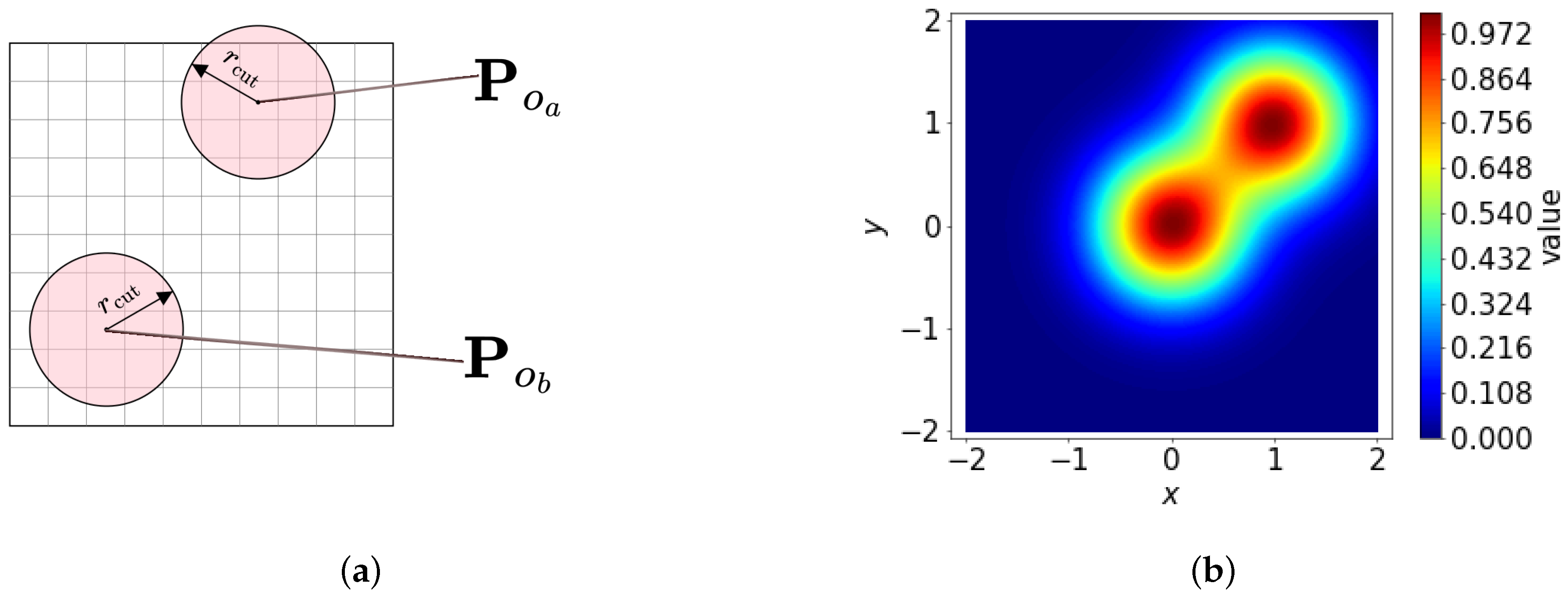
3.1.1. Density Function

We describe the local environment around a reference point ${\mathbf{r}}_o$ using a density function ${\rho }_o$, where the contributions from surrounding points within a hyperparameter $r_{\mathrm{cut}}$, are smoothly distributed through Gaussian smoothing:

$${\rho }_o(x_o,y_o,z_o)=\sum _{i}exp\left(-{\displaystyle \frac{\parallel {\mathbf{r}}_o-{\mathbf{R}}_i{\parallel }^2}{2{\sigma }_p^2}}\right),$$

(1)

where exp is the exponential function, o represents a local point, ${\mathbf{R}}_i={(x_i,y_i,z_i)}^{\top }$ are the positions of neighboring points, ${\sigma }_p$ is a hyperparameter that determines the width of the Gaussian smoothing, and ${\mathbf{r}}_o={(x_o,y_o,z_o)}^{\top }$. An example can be seen in Figure 2b.

3.1.2. Spatial Basis Function

The spatial basis function ${\Phi }_{nlm}^o(x_o,y_o,z_o)$ is defined as the product of two components: a radial function $g_{nl}^o\left(r_o\right)$ and an angular function $Y_{lm}^o({\theta }_o,{\varphi }_o)$. These components are combined as follows:

$${\Phi }_{nlm}^o(x_o,y_o,z_o)={\Phi }_{nlm}^o(r_o,{\theta }_o,{\varphi }_o)=g_{nl}^o\left(r_o\right)Y_{lm}^o({\theta }_o,{\varphi }_o),$$

(2)

where $g_{nl}^o\left(r_o\right)$ captures the radial variation, while $Y_{lm}^o({\theta }_o,{\varphi }_o)$ encodes the angular dependence in spherical coordinates, where $r_o=\sqrt{x_o^2+y_o^2+z_o^2}$ is the distance from the reference point, ${\theta }_o=arccos\left(z_o/r_o\right)$ is the polar angle, and ${\varphi }_o=arctan2(y_o,x_o)$ is the azimuthal angle (The function $\mathrm{atan}2(y,x)$ computes the angle $\theta$ between the positive x-axis and the point $(x,y)$, returning a value in $(-\pi ,\pi ]$. Unlike $arctan(y/x)$, $\mathrm{atan}2(y,x)$ accounts for the signs of both arguments to determine the correct quadrant of $\theta$). See Figure 3 as an example.

3.1.3. Radial Basis Functions

The radial basis functions $g_{nl}^o\left(r_o\right)$ capture the radial dependencies of the local environment. These functions may either depend on the angular number l (denoted as $g_{nl}^o\left(r_o\right)$) or be independent of l (denoted as $g_n^o\left(r_o\right)$). Orthonormality (A set of functions $\left\{f_i\right\}$ is orthonormal if it satisfies $\langle f_i,f_j\rangle ={\int }_a^b{f}_i\left(x\right)f_j\left(x\right)dx=0$ for $i\ne j$ (orthogonality) and $\langle f_i,f_i\rangle ={\int }_a^b{f}_i^2\left(x\right)dx=1$ (normalization)) is a key property of these basis functions, ensuring that the expansion coefficients are unique and non-redundant (See Figure 4).

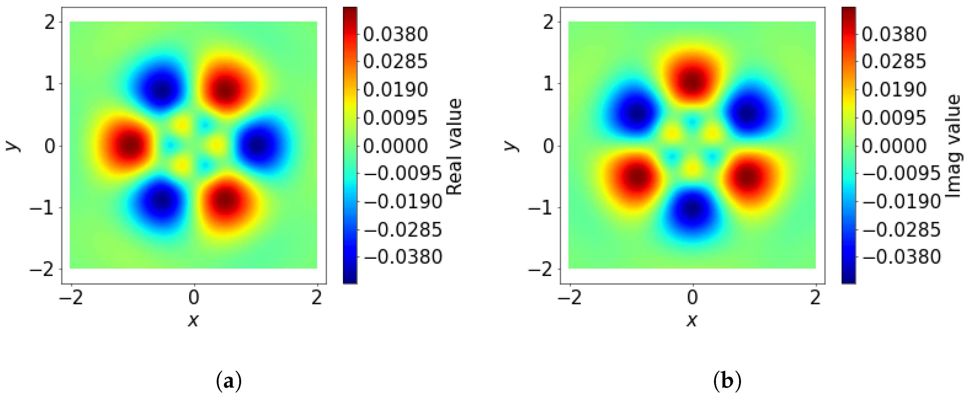
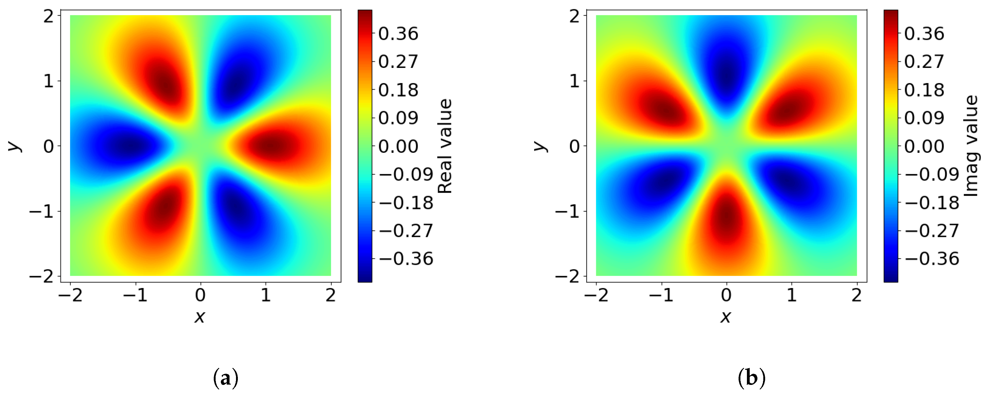
3.1.4. Angular Basis Functions

The angular basis functions $Y_{lm}^o({\theta }_o,{\varphi }_o)$ encode the angular dependencies of the local environment. These functions are constructed to represent directional information and are parameterized by two indices: l, which controls the level of angular detail, and m, which distinguishes variations within each level. This is analogous to the frequencies of sine and cosine functions around a sphere. In our case, we use spherical harmonics $Y_{lm}(\theta ,\varphi )$ as the angular basis functions (See Figure 5).

A key property of the angular basis functions is their orthonormality, ensuring that the components of the representation remain independent and non-redundant. Additionally, spherical basis functions depend only on angular coordinates, meaning they are invariant to scaling of the input vector: for any constant a,

$$Y_{lm}(x,y,z)=Y_{lm}(ax,ay,az).$$

(3)

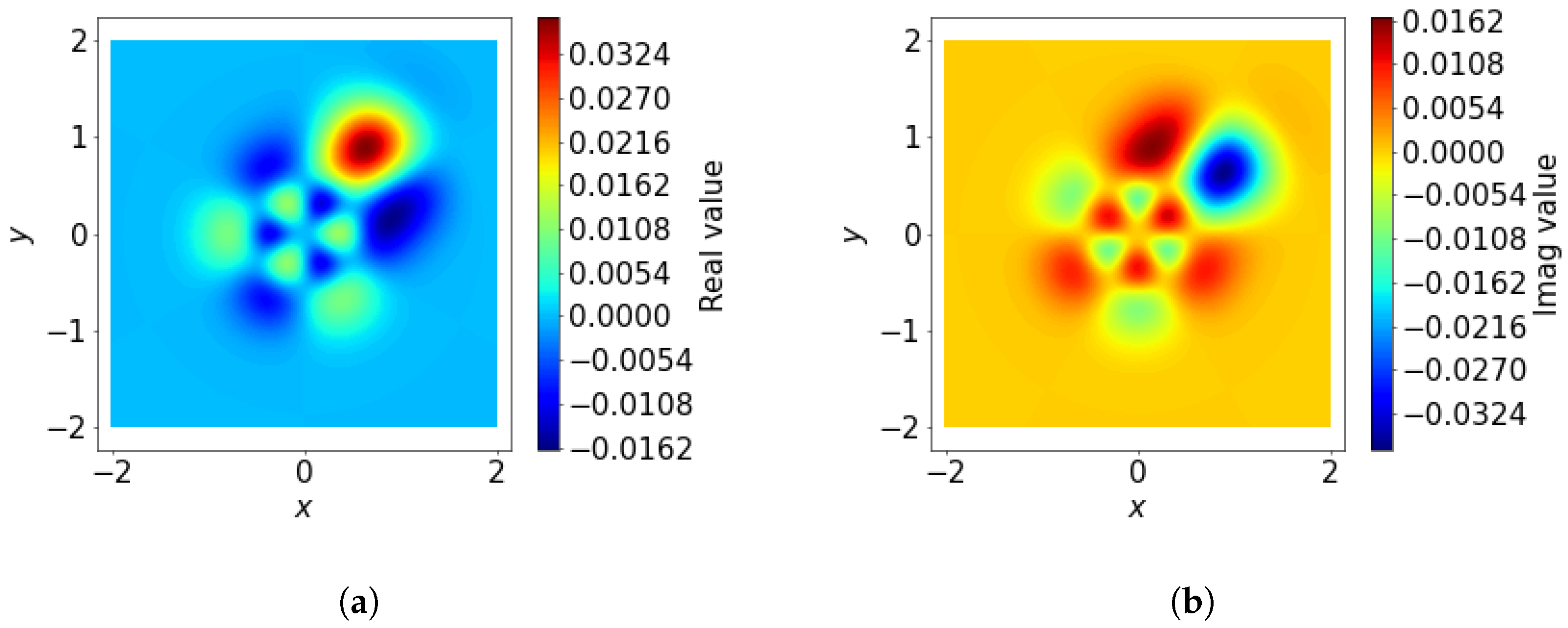
3.1.5. SOAP Expansion Coefficients

The expansion coefficients $c_{nlm}^o$ are key to representing the local environment in the SOAP formulation. These coefficients quantify the projection of the local environment density function ${\rho }_o(x_o,y_o,z_o)$ onto the spatial basis functions ${\Phi }_{nlm}^o(x_o,y_o,z_o)$, which combine radial and angular components. This projection ensures that the complex spatial information encoded in ${\rho }_o$ is transformed into a compact and expressive feature representation:

$$c_{nlm}^o={\int }_{-\infty }^{\infty }{\int }_{-\infty }^{\infty }{\int }_{-\infty }^{\infty }{\rho }_o(x_o,y_o,z_o){\Phi }_{nlm}^o(x_o,y_o,z_o)d{x}_{o}d{y}_{o}d{z}_o.$$

(4)

The orthonormality of the basis functions ensures that these coefficients are unique and non-redundant, making them an efficient and interpretable representation of the local environment. An example of an integrant is shown in Figure 6.

3.1.6. SOAP Power Spectrum

The SOAP power spectrum is a descriptor that is rotationally, translationally, and mirror invariant. It is computed as the inner product of the expansion coefficients over m, capturing the essential characteristics of the local environment. The power spectrum is defined as:

$${\mathbf{P}}_o^{\mathrm{SOAP}}=P_{n{n}^{\prime }l}^o=\pi \sqrt{{\displaystyle \frac{8}{2l+1}}}{\overline{\mathbf{c}}}_{nl}^{\top }{\mathbf{c}}_{n^{\prime }l}=\pi \sqrt{{\displaystyle \frac{8}{2l+1}}}\sum _m{\overline{c}}_{nlm}^o{c}_{n^{\prime }lm}^o,$$

(5)

where ${\overline{c}}_{nlm}^o$ is the complex conjugate of $c_{nlm}^o$. The inner product over m ensures that the power spectrum encodes information about the radial and angular dependencies while removing orientation-specific.

The resulting descriptor, ${\mathbf{P}}_o^{\mathrm{SOAP}}$, is a high-dimensional, invariant feature vector that represents the local environment around the reference point ${\mathbf{r}}_o$. This invariance is critical for tasks requiring consistent feature extraction across different orientations and positions.

A more detailed examples of the radial basis functions, angular basis functions, and coefficients, including their computation and role in feature construction, are provided in Appendix A.

3.2. Converting Images to 3D Points and Computing SOAP Descriptors

To adapt the SOAP formulation for image analysis, the pixel intensities of 2D images are converted into 3D point representations. These 3D points serve as the input for computing SOAP descriptors. This section explains the methodology for these steps.

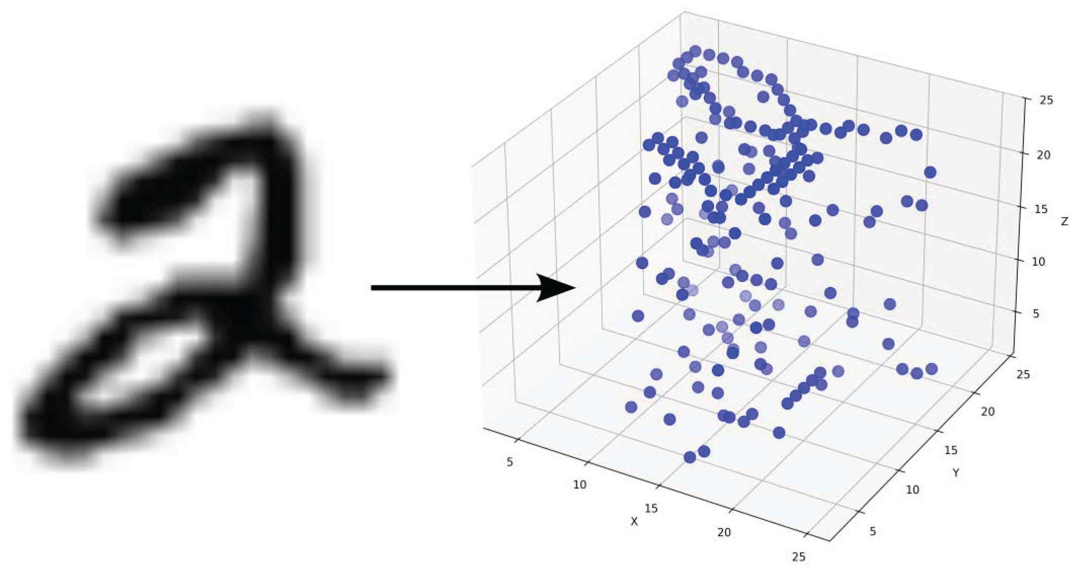
3.2.1. Converting Gray-Scale Images to 3D Points

Each image is represented as a collection of 3D points, where the x and y coordinates correspond to the pixel positions in the image, and the z-coordinate is derived from the gray-scale pixel intensity which are the values from maximum 255 divided by 10 to maximum 25.5, independent of Gaussian scaling. Algorithm 1 describes the procedure for generating the 3D representation, including an optional Gaussian displacement to account for variability or noise in the data. Variable descriptions are shown in detail in

Table A1. List of variables for SOAP descriptor computation.

Variable	Type/Dimension	Description
${\left\{{\mathbf{F}}_k\right\}}_{k=1}^n$	Collection of $N_k\times 3$ matrices	3D structure.
${\mathbf{F}}_k$	$N_k\times 3$ matrix	The k-th 3D structure containing coordinates $(x,y,z)$ of each 3D-pixel.
$\{r_{\mathrm{cut}},n_{max},l_{max},{\sigma }_p\}$	Scalars	Parameters defining the SOAP descriptor computation.
${\mathcal{P}}_k$	$N_k\times d$ matrix	SOAP descriptors for each 3D-pixel in the k-th structure.
${\mathbf{P}}_o$	$1\times d$ vector	SOAP descriptor for the o-th 3D-pixel in structure ${\mathbf{F}}_k$.
k	Integer	Index for iterating over each structure ($1\le k\le n$).
o	Integer	Index for iterating over each 3D-pixel within a structure ($1\le o\le N_k$).
${\left\{{\mathcal{P}}_k\right\}}_{k=1}^n$	Collection of $N_k\times d$ matrix	Output set of SOAP descriptors for all structures and their 3D structure.

and 

Table A2. Variables for SOAP extraction with rescaling.

Variable	Type/Dim	Description
$\mathbf{X}$	$T\times d$	Final collection of extracted and rescaled SOAP descriptors, where in our case $T=1.2\times {10}^5$ for the training data and validation data, and $T=1\times {10}^4$ for the test data.
$\mathbf{y}$	T	Labels for each row of $\mathbf{X}$.
${\mathbf{P}}_t$	$1\times d$	A single descriptor randomly chosen from ${\mathcal{P}}_r$.
${\mathbf{s}}_{RR}$	p	Robust Rescale Parameters for later use.

in Appendix B.

For a single $M_0\times M_1$ image, the intensity values of each pixel are scaled and mapped to the z-axis, while the x and y coordinates retain their pixel positions. A Gaussian displacement with standard deviation ${\sigma }_{\mathrm{disturbance}}$ is applied to the x, y, and z coordinates to introduce variability. This random displacement is particularly useful when studying the divergence of SOAP features under small perturbations. Only non-zero intensity pixels are considered in the transformation, ensuring computational efficiency by excluding irrelevant regions.

The result of this process is a 3D structure ${\mathbf{F}}_k$, where each point ${(x_i,y_i,z_i)}^{\top }$ corresponds to a pixel in the original image. This step bridges the gap between the 2D image space and the 3D local environments required for SOAP descriptor computation (Figure 7).

Algorithm 1 ConvertImagesToXYZ (3D structure)

Inputs:  ● $\left\{I_k\right\}$: A collection of n images, each of size $M_0\times M_1$, where $I_k$ is a single image.   ● ${\sigma }_{\mathrm{disturbance}}$: Standard deviation for Gaussian displacement. Outputs:  ● Points $\left\{{\mathbf{F}}_k\right\}=\left\{{(x_i,y_i,z_i)}^{\top }\right\}$ derived from the intensity values of each pixel in each image, with optional random displacement. This is the input for Algorithm 2.     1: function ImageToXYZ($I,{\sigma }_{\mathrm{disturbance}}$)       ▹ Converts a single $M_0\times M_1$ image I into 3D points. 2:     Initialize an empty list $\mathcal{P}$ for points. 3:     for $i\leftarrow 0 \mathbf{to} M_0-1$ do 4:         for $j\leftarrow 0 \mathbf{to} M_1-1$ do 5:            $z\leftarrow \lfloor I[i,j]/10\rfloor$       ▹ Squashed intensity from 255 to a scale closer to the image dimension. 6:            if $z>0$ then     ▹ Eliminated pixels that are zero 7:                $x\leftarrow j+\mathcal{N}(0,{\sigma }_{\mathrm{disturbance}}^2)$ 8:                $y\leftarrow i+\mathcal{N}(0,{\sigma }_{\mathrm{disturbance}}^2)$ 9:                $z\leftarrow z+\mathcal{N}(0,{\sigma }_{\mathrm{disturbance}}^2)$ 10:              Append $(x,y,z)$ to $\mathbf{F}$. 11:            end if 12:         end for 13:     end for 14:     return $\mathbf{F}$ 15: end function        ▹ Main procedure: convert all images $\left\{I_k\right\}$ into 3D point sets. 16: for $k\leftarrow 1 \mathbf{to} n$ do 17:     ${\mathbf{F}}_k\leftarrow$ImageToXYZ $(I_k,{\sigma }_{\mathrm{disturbance}})$ 18: end for

3.2.2. Computing SOAP Descriptors for Image 3D Structures

Once the images are converted into 3D structures, SOAP descriptors are computed for each point in the 3D space. Algorithm 2 provides a detailed procedure for this computation. Each 3D structure ${\mathbf{F}}_k$ is processed to extract per-point SOAP descriptors, capturing the local spatial arrangement of points.

For each point ${\mathbf{r}}_o={(x_o,y_o,z_o)}^{\top }$ in ${\mathbf{F}}_k$, the SOAP formulation outlined earlier is applied. Using the radial basis functions $g_{nl}^o\left(r_o\right)$ and angular basis functions $Y_{lm}^o(\theta ,\varphi )$, the density function is expanded into orthonormal basis functions. The expansion coefficients $c_{nlm}^o$ are then used to compute the power spectrum ${\mathbf{P}}_o^{\mathrm{SOAP}}$ as described in Equation (6).

The result is a matrix ${\mathcal{P}}_k$, where each row represents the SOAP descriptor ${\mathbf{P}}_o$ for a single point in the 3D structure. The descriptors encode local spatial patterns in a manner invariant to rotations, translations, and mirror symmetry. By aggregating the SOAP descriptors across all points, a comprehensive feature set for the image is obtained, enabling pixel-wise classification and other machine learning tasks.

This approach leverages the robustness of SOAP descriptors to provide a high-dimensional, invariant representation of image features, merging methodologies from quantum chemistry and computer vision.

Algorithm 2 Compute SOAP Matrices for a Set of 3D Structures

Inputs:  ● A collection of 3D structures ${\left\{{\mathbf{F}}_k\right\}}_{k=1}^n$, where each structure ${\mathbf{F}}_k$ is an $N_k\times 3$ matrix containing coordinates in 3D space: $${\mathbf{F}}_k=\left(\begin{array}{ccc}{x}_1& y_1& z_1\\ x_2& y_2& z_2\\ ⋮& ⋮& ⋮\\ x_{N_k}& y_{N_k}& z_{N_k}\end{array}\right).$$   ● Parameters for the SOAP descriptor: $\{r_{\mathrm{cut}},n_{max},l_{max},{\sigma }_p\}$. Outputs:  ● A set of SOAP matrices ${\left\{{\mathcal{P}}_k\right\}}_{k=1}^n$, where each ${\mathcal{P}}_k$ is an $N_k\times d$ matrix holding the per-point SOAP vectors $\left\{{\mathbf{P}}_o\right\}$ for ${\mathbf{F}}_k$. In other words, $${\mathcal{P}}_k=\left(\begin{array}{c}{\mathbf{P}}_{o1}\\ {\mathbf{P}}_{o2}\\ ⋮\\ {\mathbf{p}}_{o{N}_k}\end{array}\right),{\mathbf{P}}_o\in {\mathbb{R}}^d.$$   This will be the input for Algorithm 3.                     ▹Algorithm Steps 1: Initialize an empty set ${\left\{{\mathcal{P}}_k\right\}}_{k=1}^n$ store all SOAP matrices. 2: for  $k\leftarrow 1 \mathbf{to} n$ do 3:     Let ${\mathbf{F}}_k$ be of size $(N_k\times 3)$. 4:     Define ${\mathcal{P}}_k$ as an $(N_k\times d)$ matrix. 5:     for $o\leftarrow 1\mathbf{to}{N}_k$ do       ▹ Compute SOAP vector ${\mathbf{P}}_o$ for the o-th point of structure ${\mathbf{F}}_k$. 6:         ${\mathbf{P}}_o\leftarrow \mathrm{SOAP}\left({\mathbf{F}}_k;r_{\mathrm{cut}},n_{max},l_{max},{\sigma }_p\right)$       ▹ Compute SOAP Spectra for each non-zero pixel. 7:         Insert ${\mathbf{P}}_o$ (a $1\times d$ vector) into the o-th row of ${\mathcal{P}}_k$. 8:     end for 9:     Store ${\mathcal{P}}_k$ in the overall result set ${\left\{{\mathcal{P}}_k\right\}}_{k=1}^n$. 10: end for 11: return ${\left\{{\mathcal{P}}_k\right\}}_{k=1}^n$    ▹ Each ${\mathcal{P}}_k$ is a matrix capturing SOAP descriptors of ${\mathbf{F}}_k$.

Algorithm 3 Random Extraction of SOAP Spectra with Rescaling

Inputs:  Collection of SOAP vectors from 3D structures, ${\left\{{\mathcal{P}}_k\right\}}_{k=0}^{N_k-1}=\{{\mathcal{P}}_0,\dots ,{\mathcal{P}}_{N_k-1}\}$. Outputs:  Extracted and rescaled SOAP descriptors $\mathbf{X}\in {\mathbb{R}}^{T\times d}$, and corresponding labels $\mathbf{y}\in {\mathbb{R}}^T$ with the rescaler ${\mathbf{s}}_{R}R$. This will be the dataset for the experiments.     1: Initialize $\mathbf{X}\leftarrow {\mathbf{0}}_{T\times d}$ 2: Initialize $\mathbf{y}\leftarrow {\mathbf{0}}_T$ 3: for  $t\leftarrow 1$ to T do 4:     Pick a random index $r\in \{0,\dots ,N_k-1\}$ 5:     Select a random descriptor ${\mathbf{P}}_t\in {\mathbb{R}}^d$ from file ${\mathcal{P}}_r$ 6:     $\mathbf{X}[t,:]\leftarrow {\mathbf{P}}_t$ 7:     $\mathbf{y}\left[t\right]\leftarrow {\ell }_r$ 8: end for 9: $(\mathbf{X},{\mathbf{s}}_{RR})\leftarrow \mathrm{RobustRescalor}\left(\mathbf{X}\right)$ 10: return  $\mathbf{X},\mathbf{y},{\mathbf{s}}_{RR}$

4. Experiments and Results

To evaluate the performance of SOAP-based pixel-wise classification, a series of experiments were conducted. This section details the creation of the training datasets and outlines the experimental setups used to validate the methodology.

To systematically assess the effectiveness of SOAP-based pixel-wise classification, we conduct three key experiments. The first experiment focuses on hyperparameter optimization and pixel predictions, where we explore the impact of various SOAP descriptor parameters on model performance to determine an optimal configuration, then predict their classification of each pixel on the validation and test set. The second experiment investigates SOAP vector compression, evaluating different dimensionality reduction techniques—including PCA, linear autoencoding, and deep autoencoding—to quantify the trade-off between compression and classification accuracy. Finally, the third experiment examines robustness to pixel position perturbations, introducing Gaussian noise to pixel coordinates to assess the stability of SOAP-based feature extraction in the presence of spatial distortions.

4.1. Training Data Preparation

The training data for the experiments was derived from the SOAP descriptors computed for the 3D structures obtained from the MNIST dataset of handwritten digits. This dataset consists of 60,000 gray-scale images of size $28\times 28$ pixels. Each image was converted into a 3D structure following the methodology described in Section 3.2. 120,000 random SOAP spectra were collected, and split into 0.8:0.2 training and validation sets. The test dataset was collected from the MNIST handwritten dataset of 10,000 gray-scale images, and 10,000 random SOAP spectra were collected as a test set. The processes for generating the datasets in each experiment are detailed in Algorithm 3.

As for the training and validation, a collection of SOAP matrices, ${\left\{{\mathcal{P}}_k\right\}}_{k=0}^{N_k-1}$, was computed using the Dscribe Python, package, version 2.1.1 [6,24] and then randomly sampled to extract $T=12\times {10}^4$ descriptors. These descriptors form the training feature matrix $\mathbf{X}\in {\mathbb{R}}^{T\times d}$. Each SOAP vector ${\mathbf{P}}_t$ was assigned a corresponding label ${\ell }_r$, indicating its association with the r-th digit class in the MNIST dataset.

By using the MNIST dataset, this study leverages the well-established benchmark for handwritten digit recognition, enabling a rigorous evaluation of the proposed methodology and facilitating comparisons with other approaches.

To ensure numerical stability and facilitate model convergence, the SOAP descriptors were rescaled using a robust rescaling procedure, RobustRescalor, which adjusts the data based on the distribution of feature values. The rescaled descriptors and their corresponding labels constitute the final dataset, $(\mathbf{X},\mathbf{y})$, with the parameters for robust rescaling for later use ${\mathbf{s}}_{RR}$ used in subsequent experiments.

The creation of this dataset ensures diversity in the sampled descriptors and maintains a balanced representation across the different input structures, facilitating robust model training and evaluation.

4.2. Experiment 1: Hyperparameter Optimization for SOAP and Predictions

4.2.1. Objective

The objective of this experiment is to identify the optimal SOAP descriptor parameters ($r_{\mathrm{cut}}$, $n_{\max }$, $l_{\max }$, and ${\sigma }_p$) for pixel-wise digit classification and to evaluate their impact on model performance. This experiment aims to establish the sensitivity of the model to these parameters and determine the configurations that maximize validation accuracy while minimizing redundancy.

4.2.2. Methods

In this experiment, we employed a hyperparameter search using a Monte Carlo sampling strategy [25] over 168 trials. Monte Carlo sampling refers to a probabilistic technique where values are drawn randomly from specified distributions rather than systematically exploring all possible combinations (as in grid search). This approach allows for efficient exploration of high-dimensional hyperparameter spaces by sampling diverse configurations, reducing the computational cost associated with exhaustive search. 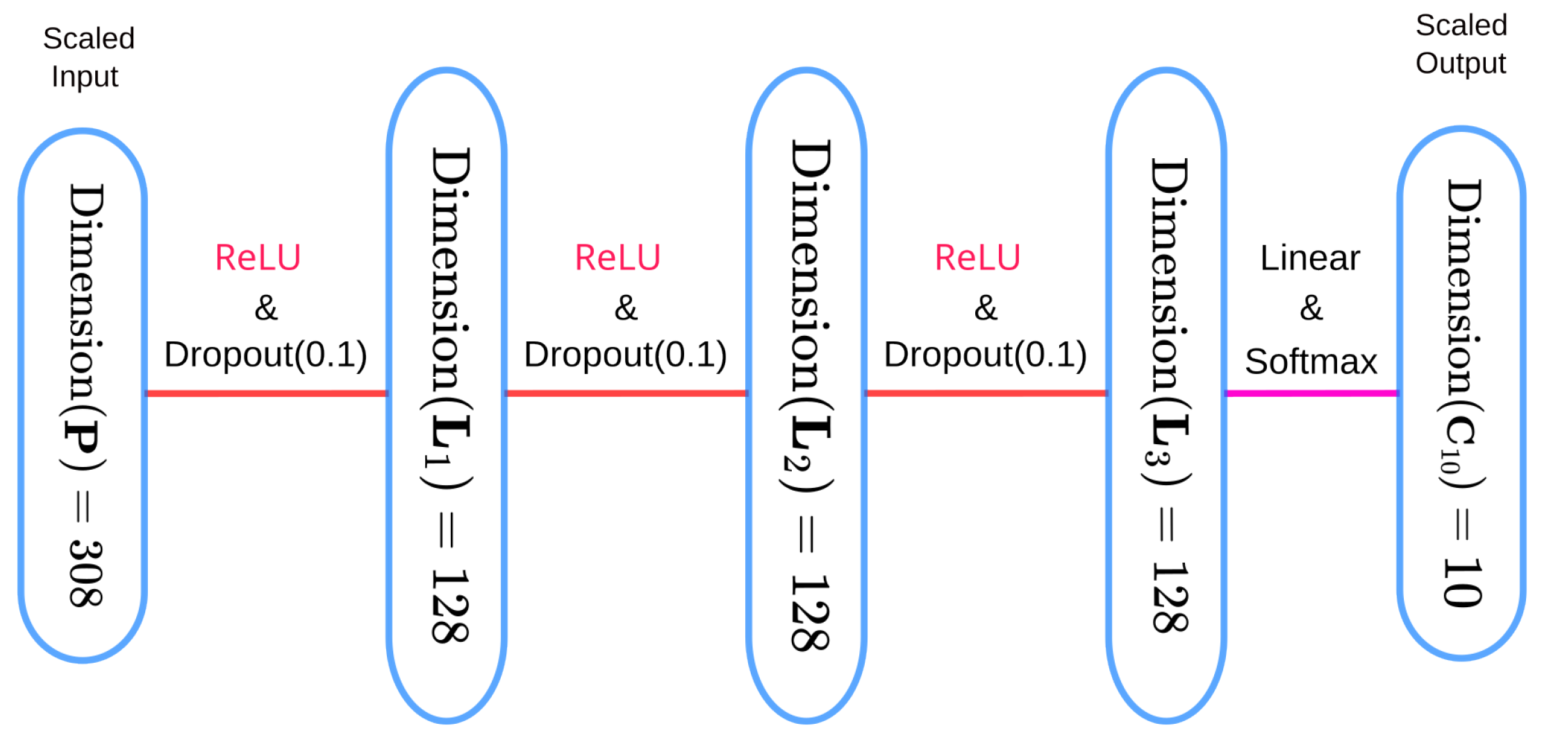The search explored the following ranges: the neighborhood radius $r_{\mathrm{cut}}$ was varied between 2 and 100, the radial basis count $n_{\max }$ between 2 and 11, the angular resolution $l_{\max }$ between 2 and 11, and the Gaussian width ${\sigma }_p$ between 1 and 10. The model architecture used was the pixel-wise classification model (see Figure 8), trained on 120,000 data points consisting of SOAP descriptors derived from MNIST images. The training protocol included the Adam optimizer [26] with a learning rate of 0.001, a batch size of 128, and 300 training epochs, with the data split into 80% for training and 20% for validation. Validation accuracy served as the primary metric, and the influence of individual hyperparameters was analyzed by correlating them with accuracy trends across the trials.

4.2.3. Results

The best combination of hyperparameters, listed in Table A1, yielded a validation accuracy of 0.6844. Notably, $r_{\mathrm{cut}}$ exerted the greatest influence on accuracy, while ${\sigma }_p$ performed best between 2 and 5. The parameters $n_{\max }$ and $l_{\max }$ had less impact, provided they were larger than approximately 6. The size of the pixel-wise SOAP spectra with the optimal parameters was $7(7+1)/2\times (10+1)=308$. The results are summarized in

Table 1. Test values for the optimal hyperparameters found by Monte Carlo search using validation accuracy as benchmark. The parameters found are $r_{\mathrm{cut}}=63$, $n_{\max }=7$, $l_{\max }=10$, ${\sigma }_p=3$. The validation accuracy yielded 0.6844 while test accuracy yielded 0.6863.

Accuracy	Recall	Precision	F1 Score
0.6863	0.6863	0.6821	0.6832

and the confusion matrix on the test set is shown in Figure 9. Figure 10 presents scatter plots illustrating the relationships between the different hyperparameters ($n_{\max }$, $l_{\max }$, $r_{\mathrm{cut}}$, and ${\sigma }_p$) and their effect on validation accuracy.

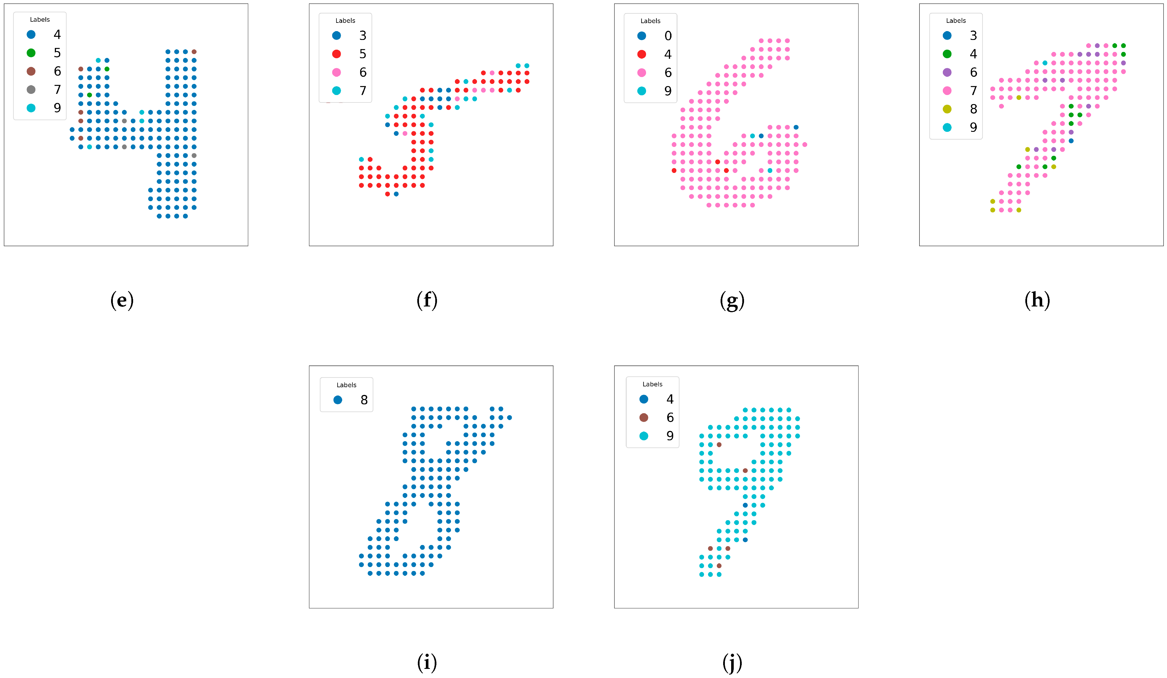
Figure 11 shows examples of handwritten digits that are relatively easy to classify, indicating near-perfect predictions on clear and unambiguous shapes. These images highlight situations where SOAP-based features can successfully capture local environments without requiring additional data augmentation (e.g., rotation or flipping).

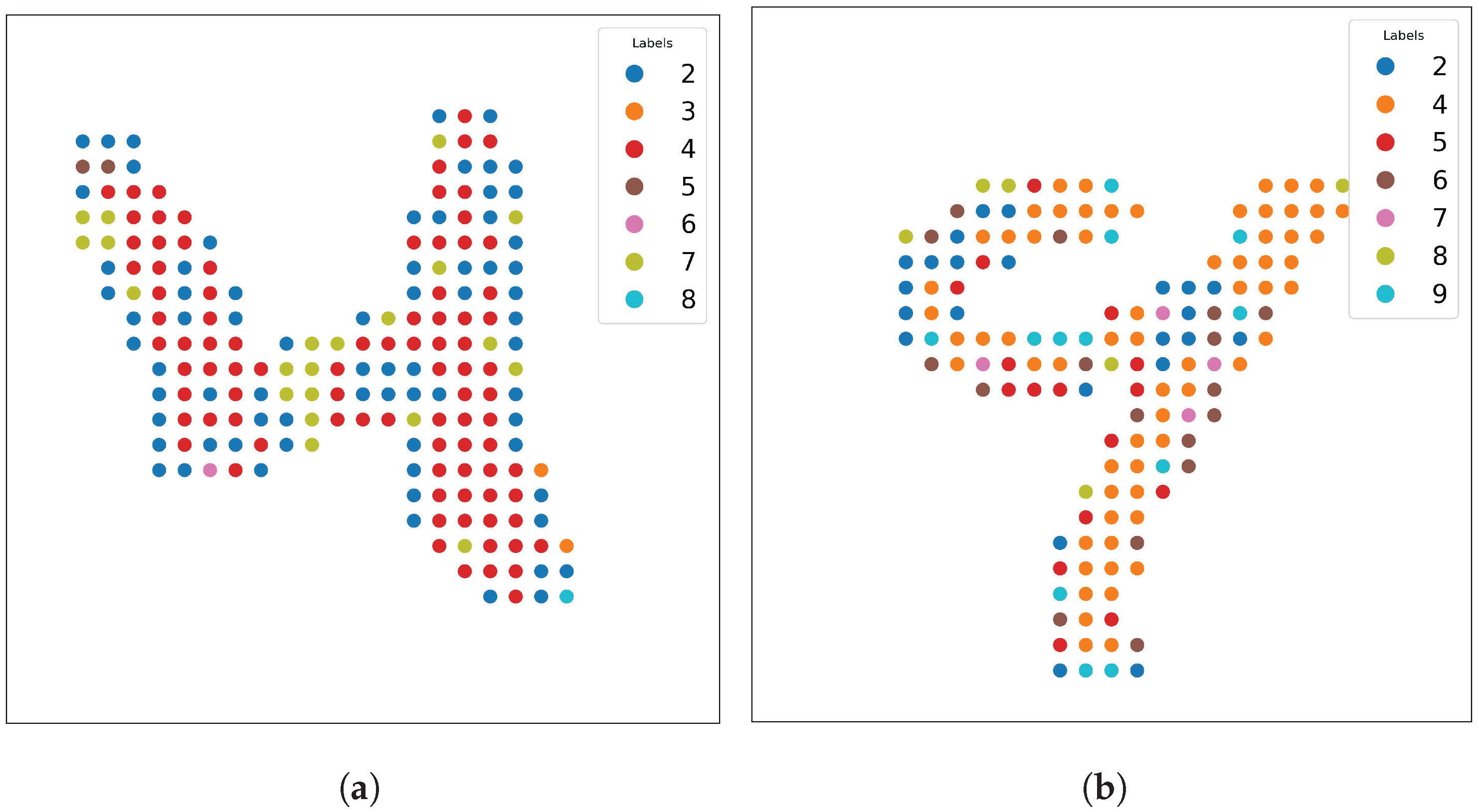
Figure 12 demonstrates a challenging case where a handwritten 7 (Figure 12a) can be rotated 90 degrees and mirror-flipped (Figure 12b), causing the model to misclassify it as a 4. This misclassification arises because SOAP features do not inherently distinguish between these symmetries.

Figure 13 displays another example where points far from the handwritten shape (digit 3) tend to be predicted less accurately. These edge points do not strongly resemble any digit, indicating that SOAP features, while robust, still depend on local geometry and can produce errors on pixels far from the number’s main structure.

Finally, Figure 14 shows ambiguous shapes of handwritten digits (e.g., a 4 and a 9) that can confuse not only the model but also human observers. In such cases, even the most sophisticated feature extraction approaches may fail if the digit is too ambiguous.

4.2.4. Discussion

The results underscore the importance of selecting an appropriate $r_{\mathrm{cut}}$ and ensuring ${\sigma }_p$ lies in the range of 2–5 for improved accuracy. By leveraging SOAP features, our model does not require augmentation for training, such as rotation, translation, or mirror flipping. This is because SOAP naturally encodes local geometric information of each pixel or point in the handwritten digits.

However, the same property that makes SOAP robust against certain transformations also introduces challenges when symmetrical orientations are key to correct identification. For instance, as shown in Figure 12, a handwritten digit 7 rotated 90 degrees and mirror-flipped closely resembles a 4. Humans also tend to misinterpret it in such an orientation [27], but in deep learning-based models without built-in symmetry handling, such misclassifications can be frequent. Moreover, SOAP struggles with highly ambiguous handwriting (see Figure 14), although this limitation is not unique to SOAP.

Computational cost must also be taken into account, as the pipeline introduces additional steps not present in typical CNN-based methods—such as the conversion of image data into 3D point clouds and the calculation of SOAP descriptors, which involve relatively high computational complexity (see Appendix A).

In summary, SOAP-based feature extraction presents a strong option for digit classification tasks, particularly for reducing the need for data augmentation. It is especially effective for clear, unambiguous shapes and for learning from relatively limited data. Yet, there are limitations for SOAP (e.g., not being able to distinguish between 6 and 9 sometimes due to rotational invariance), and additional strategies to account for orientation or symmetries may be required to further improve accuracy.

4.3. Experiment 2: SOAP Vector Compression and Impact on Prediction Accuracy

4.3.1. Objective

The high-dimensional nature of SOAP descriptors (308 dimensions in our optimal configuration) introduces computational challenges for downstream machine learning tasks. This experiment evaluates the compressibility of SOAP vectors by comparing three encoding methods—principal component analysis (PCA), linear autoencoding, and deep autoencoding—and quantifies the trade-off between compression ratio and reconstruction accuracy. We further analyze how compression impacts the performance of digit classification.

4.3.2. Methods

For this experiment, we use a subset of 120,000 SOAP descriptors from Experiment 1, which is divided into training (80%) and validation (20%) sets. The compression techniques considered include PCA, which performs linear dimensionality reduction via singular value decomposition; a linear autoencoder, implemented as a single-layer neural network with $h_e$ hidden units and linear activation (see Figure 15); and a deep autoencoder, which employs a non-linear architecture with an encoder defined as $f_e:{\mathbb{R}}^{308}\to {\mathbb{R}}^{308h_m}\to {\mathbb{R}}^{h_e}$ and a decoder defined as $f_d:{\mathbb{R}}^{h_e}\to {\mathbb{R}}^{308h_m}\to {\mathbb{R}}^{308}$, where $h_m\in \{2,4,10\}$ controls the hidden layer capacity (see Figure 16). The evaluation metrics include the reconstruction loss, measured as the mean squared error (MSE) [28] between the original and reconstructed SOAP vectors, and the classification accuracy of Model A (from Experiment 1) when using the compressed features. All autoencoders are implemented using the Adam optimizer with a learning rate of 0.0001 and a batch size of 512, and they are trained for 10,000 epochs.

4.3.3. Results

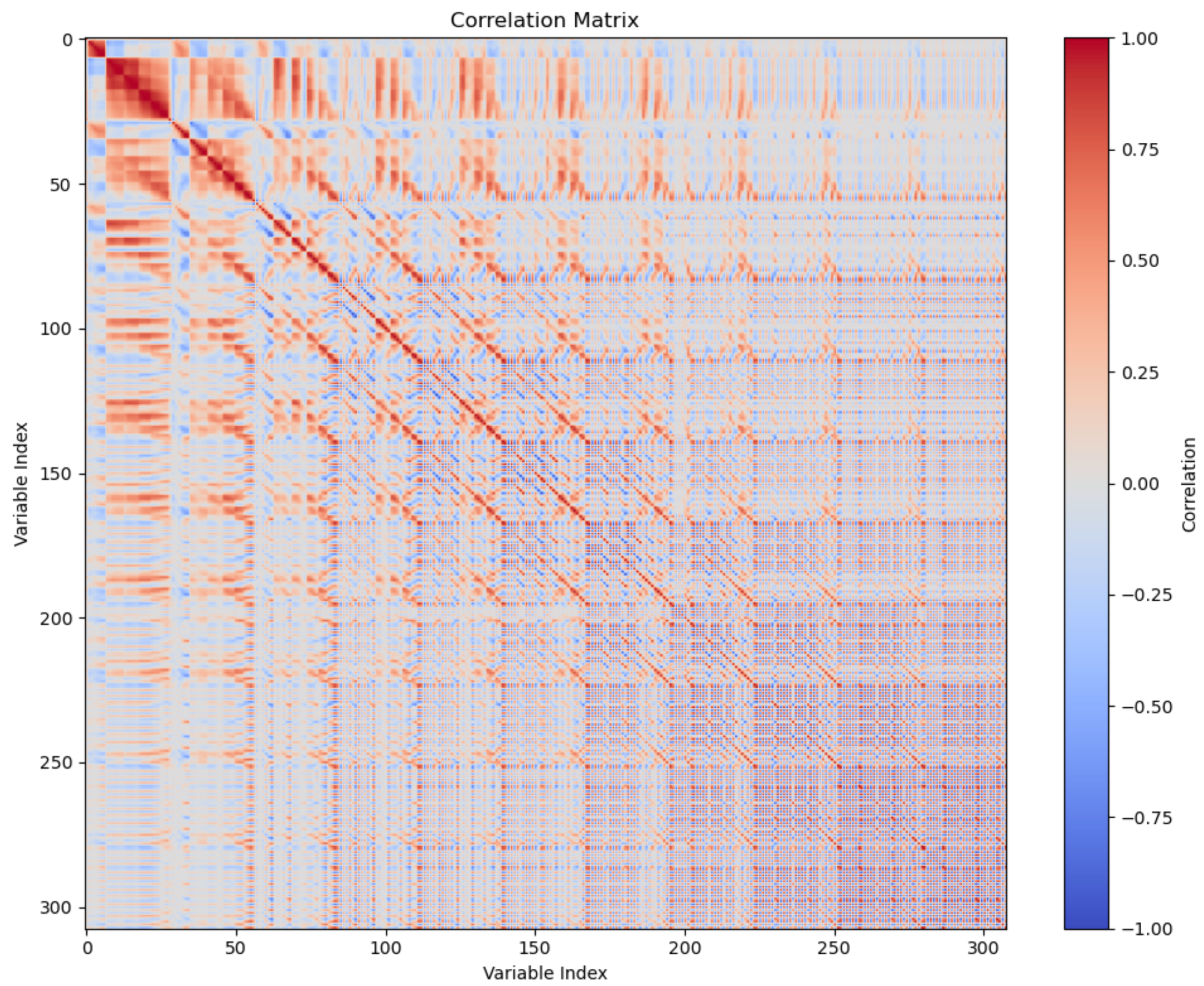
Figure 17 reveals strong correlations between SOAP vector components, suggesting significant redundancy and motivating compression to eliminate redundant dimensions without sacrificing predictive power. Figure 18 shows the relationship between the encoding dimension $h_e$ and the reconstruction loss, where both PCA and a linear autoencoder exhibit identical performance for $h_e<200$, with PCA becoming superior at higher dimensions due to its optimal linear subspace identification, while a deep autoencoder outperforms linear methods for $h_e<50$ by leveraging non-linear mappings to preserve information. 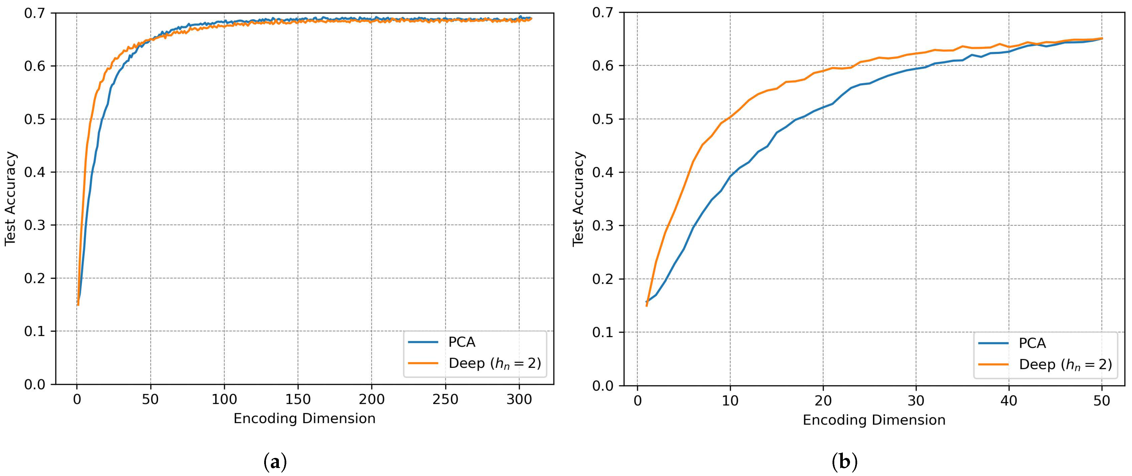Furthermore, Figure 19 demonstrates the impact of compression on classification accuracy: for high dimensions ($h_e>50$), all methods achieve more than 95% of the baseline accuracy (308 dimensions), with PCA slightly outperforming autoencoders, whereas under aggressive compression ($h_e<50$), test accuracy suddenly drops and deep autoencoding outperforms PCA.

4.3.4. Discussion

SOAP vectors exhibit substantial redundancy, enabling compression to approximately 100 dimensions (one-third of the original size) without any loss in accuracy. The key findings include computational efficiency—since principal component analysis (PCA) provides optimal compression for $h_e>50$, requiring no training and minimal implementation effort—and performance in the high compression regime, where deep autoencoders outperform linear methods for $h_e<50$, albeit at the cost of increased model complexity. Moreover, for MNIST classification, compressing to $h_e=100$ results in nearly no loss in prediction accuracy (98% of the baseline). This analysis confirms that SOAP’s rotational and translational invariance does not preclude efficient compression, and it indicates that the choice between linear and non-linear compression depends on the target dimensionality and acceptable accuracy trade-offs. Future work could explore hybrid approaches or task-specific compression to further optimize this balance.

4.4. Experiment 3: Robustness to Pixel Position Perturbations

4.4.1. Objective

To evaluate the robustness of SOAP-based feature extraction against noise, we introduce Gaussian perturbations to pixel positions and measure the impact on validation accuracy. This experiment tests whether the method gracefully degrades with increasing noise, thereby reflecting its stability in real-world scenarios with imperfect data.

4.4.2. Methods

In our approach, noise is injected into each image by perturbing the pixel coordinates $(x,y)$ and the intensity-derived z-values with additive Gaussian noise according to the equation

$${\mathbf{r}}_i^{\prime }={\mathbf{r}}_i+ϵ,ϵ\sim \mathcal{N}(0,{\sigma }_{\mathrm{disturbance}}^2\mathbf{I}),$$

where ${\sigma }_{\mathrm{disturbance}}$ controls the noise magnitude (tested over a range from $0.1$ to $5.0$ in 20 logarithmic steps). The dataset consists of 10,000 MNIST test images converted to 3D structures with noise using the same SOAP parameters as in Experiment 1 ($r_{\mathrm{cut}}=63$, $n_{\max }=7$, $l_{\max }=10$, ${\sigma }_p=3$), and the model employed is our three-layer prediction model (see Figure 8). The primary metric for evaluation is the validation accuracy as a function of ${\sigma }_{\mathrm{disturbance}}$.

4.4.3. Results

The results, as shown in Figure 20, indicate that validation accuracy decreases smoothly with increasing ${\sigma }_{\mathrm{disturbance}}$. At a noise level of ${\sigma }_{\mathrm{disturbance}}=1.0$, accuracy remains at 92% of the baseline (i.e., the case when ${\sigma }_{\mathrm{disturbance}}=0$), demonstrating robustness to moderate noise; however, performance drops to chance levels (approximately 51%) at ${\sigma }_{\mathrm{disturbance}}=3.9$, a point where local pixel neighborhoods are irrecoverably distorted. Additionally, a critical threshold is observed: accuracy declines sharply beyond ${\sigma }_{\mathrm{disturbance}}=0.5$.

4.4.4. Discussion

These findings demonstrate that SOAP-based features exhibit gradual performance degradation under controlled noise, confirming their stability for practical applications. The smooth decline in accuracy, rather than a catastrophic failure, validates the method’s suitability for scenarios with noisy data and positional uncertainty, and suggests that future work could couple SOAP with denoising techniques to further enhance robustness.

4.5. Experiment 4: Comparison of SOAP and CNN Under Rotation Augmentation

4.5.1. Objective

The objective of this experiment is to compare the performance of SOAP descriptors and CNN-based models under rotation-based data augmentation. Specifically, we evaluate how both approaches perform when trained on datasets with and without rotation augmentation and tested on uniformly rotated versions of the MNIST dataset.

4.5.2. Methods

Two training datasets were constructed from the MNIST handwritten digits training set. For the first dataset, we randomly selected 6000 images and applied random in-plane rotations between 0 and 360 degrees. From each rotated image, a local patch of size $15\times 15$ pixels was extracted, centered on a pixel with a non-zero value to ensure the region contained part of a digit.

The second training dataset consisted of 6000 samples selected in the same manner, but without applying any rotation. In both cases, the local patches were cropped from the original $28\times 28$ images.

The test set consisted of 10,000 local $15\times 15$ patches extracted from the MNIST test set. Each test image was randomly rotated between 0 and 360 degrees. Importantly, in all cases, only the center pixel of each $15\times 15$ patch was used for label prediction. For the SOAP model, this means that a SOAP spectrum was computed exclusively at the center of each local image region, corresponding to the pixel to be classified.

SOAP descriptors were parameterized as in Experiment 1: $r_{\mathrm{cut}}=42$, $n_{\max }=5$, $l_{\max }=10$, and ${\sigma }_p=2$.

For the CNN baseline, we used a standard architecture comprising two convolutional layers followed by fully connected layers. The network consisted of: a convolutional layer with 16 filters of size $3\times 3$, followed by ReLU activation and $2\times 2$ max pooling; a second convolutional layer with 32 filters of size $3\times 3$, again followed by ReLU activation and $2\times 2$ max pooling; a flattening step; a fully connected layer with 64 hidden units and ReLU activation; and finally, a 10-way softmax output layer for classification. This network operates directly on the $15\times 15$ image patches.

Training was performed with an 80:20 train–validation split, using a batch size of 2048, a learning rate of 0.0001, and for 1000 epochs. Testing was conducted using the model that achieved the best validation accuracy. Results were averaged over 10 independent runs to reduce variance. Performance was evaluated by incrementally increasing the training set size from 100 to 6000 samples, in steps of 100.

4.5.3. Results

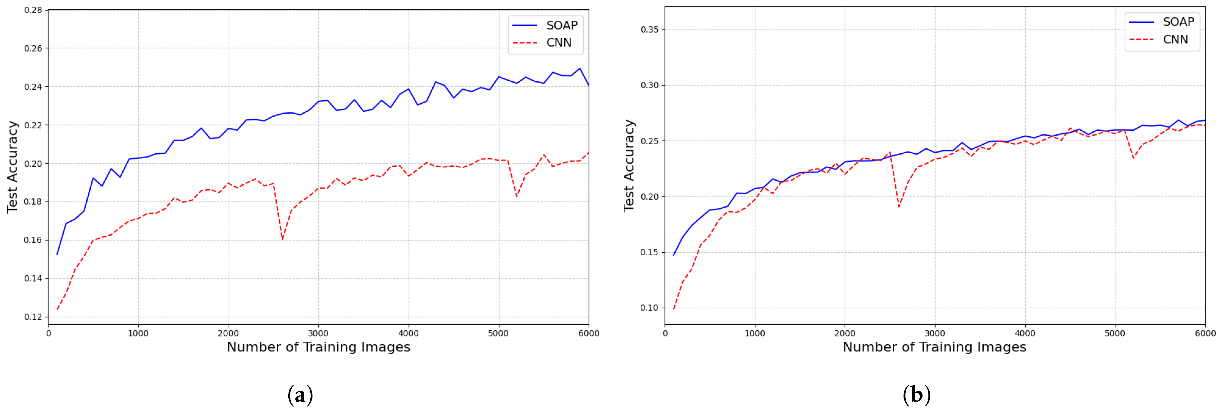
Figure 21 shows the test accuracy curves for both the SOAP and CNN models under the two training conditions: (a) training without rotation augmentation, and (b) training with rotation augmentation. Each point on the curve represents the average test accuracy over 10 independent runs.

4.5.4. Discussion

The results clearly show that when the training set does not include rotation augmentation, the SOAP model significantly outperforms the CNN model on rotated test images. This supports the idea that SOAP inherently encodes rotational invariance, reducing the need for explicit augmentation.

However, when both models are trained with rotation-augmented data, their performance becomes comparable for training sizes larger than approximately 1000 samples. This demonstrates that CNNs can learn rotational robustness with sufficient data and augmentation, although at the cost of requiring more training samples and additional data augmentation.

While this experiment used simple geometric augmentation (in-plane rotation) on a relatively clean dataset, in real-world applications such transformations are often more complex and difficult to engineer. In such cases, the invariance properties of SOAP could offer practical advantages. That said, the computational cost of SOAP—including the conversion of each local patch into a 3D point cloud and the evaluation of the descriptor—must be taken into account (see Appendix A).

5. Future Work

While this study has demonstrated the potential of SOAP-based descriptors for pixel-wise classification as a benchmark, several extensions and improvements can be explored in future work. One intriguing direction is the adaptation of SOAP for RGB images rather than gray-scale. Since SOAP includes species as a hyperparameter, different channels of an RGB image could be encoded using distinct species. For instance, one could draw an analogy by assigning the red, green, and blue channels to chemical species such as hydrogen (H), helium (He), and lithium (Li), respectively. This approach may introduce a richer feature space by allowing inter-channel interactions to be represented in a way similar to multi-species atomic environments.

Another key limitation of SOAP is its inherent invariance to symmetry transformations, which may discard crucial orientation-dependent information. To address this, a strategy of forced symmetry breaking could be employed. One possible method is to introduce auxiliary points near each pixel, such as a structured line below a handwritten digit, to provide directional context. This additional information could help encode spatial orientation, enabling the descriptors to retain some asymmetry where needed.

Beyond pixel-wise classification, future work could explore leveraging SOAP vectors to construct global representations for entire images. For example, one could compute an aggregate representation by averaging SOAP vectors across all pixels in an image, creating a holistic descriptor that remains invariant yet captures key structural patterns. Alternatively, more sophisticated approaches such as graph neural networks could be applied to learn higher-order relationships between SOAP descriptors, potentially enhancing performance in global classification tasks.

Additionally, in this study, we utilized the SOAP power spectrum, which provides a robust yet relatively compact representation of local environments. However, SOAP also offers a more expressive addition known as the bispectrum, which retains higher-order structural correlations and can encode more intricate geometric details. Future work could investigate whether incorporating the SOAP bispectrum leads to improved classification performance, particularly in tasks where capturing finer structural nuances is critical.

Finally, another potential avenue is the direct application of SOAP-based descriptors to point cloud classification tasks. Given that SOAP was originally designed for atomic-scale modeling, its extension to three-dimensional point clouds in computer vision could be a natural progression. This could involve adapting SOAP to tasks such as 3D object recognition, scene reconstruction, or LiDAR data analysis, where local geometric structures play a crucial role in classification.

These directions illustrate the versatility of SOAP-based feature extraction and open up exciting possibilities for extending its applications beyond gray-scale image classification to more complex and structured data representations.

6. Conclusions

In this work, we have demonstrated how the Smooth Overlap of Atomic Positions (SOAP), originally developed for atomic-scale modeling in chemistry and materials science, can be adapted to extract pixel-wise descriptors for images. By viewing each pixel as a local “environment” and lifting 2D image data into 3D space, we obtain SOAP vectors that capture rich local structure while maintaining invariance to translation, rotation, and mirror symmetry. One of the primary strengths of this method is that it obviates the need for extensive data augmentation for these transformations, allowing us to train models effectively without having to create or include rotated, translated, or mirrored variants of the input images. However, if mirror-flipping information (or other orientation-dependent cues) is intrinsically relevant to the classification task, SOAP’s invariant nature can become a limitation, since it effectively discards such distinguishing orientation-specific features, such as distinguishing between the numbers 6 and 9.

Our experiments on MNIST show that careful tuning of SOAP hyperparameters, especially the cutoff radius, is critical for optimal classification performance. Furthermore, we have illustrated the high compressibility of SOAP features via PCA and autoencoders, reducing dimensionality without significantly degrading predictive accuracy. We also investigated the robustness of SOAP-based descriptors to positional noise. Perturbing the pixel coordinates with Gaussian noise revealed a smooth decline in accuracy, confirming that SOAP gracefully handles moderate spatial uncertainties. This resilience is valuable for real-world datasets where image acquisition or labeling may be imperfect.

A major strength of this approach is its general applicability to any set of data points that can be projected into 3D space. Beyond images, the same pipeline can potentially be readily applied to diverse domains such as 3D object recognition, geospatial data analysis, or even higher-dimensional biomedical images where pixel or voxel intensities can be mapped into spatial coordinates. By combining inherent invariance, robust local feature encoding, and flexible dimensionality reduction, SOAP-based descriptors provide a framework for learning tasks that rely on capturing local patterns in a manner invariant to common image transformations. The results presented here open a potential avenue for future work in computer vision and related fields, where the capacity to incorporate sophisticated descriptors from quantum chemistry can lead to robust, efficient, and interpretable representations.