Hysteresis in Neuron Models with Adapting Feedback Synapses


Abstract
1. Introduction
2. Continuous Neuron Models with Adapting Feedback Synapse
3. Discrete Neuron Models with Adapting Feedback Synapse
4. Conclusions
Author Contributions
Funding
Institutional Review Board Statement
Informed Consent Statement
Data Availability Statement
Acknowledgments
Conflicts of Interest
Appendix A
| % MATLAB Program. |
| % See Figure 2. Animated Single Neuron with Adaptive Synapse. |
| % Start with u=-0.1 and s=1. |
| % Plot the single trajectory as the parameter alpha goes from 0 to 5. |
| clear |
| clear |
| xa=zeros(10000); |
| xmin=-0.2;xmax=0.2; |
| ymin=0.2;ymax=2.6; |
| q=5;p=5;epsilon=0.2;w=2*pi; |
| t_int=500; |
| for j=1:500 |
| F(j)=getframe; |
| alpha=0.01*j; |
| sys = @(t,x) [-x(1)+f1(q*x(2))*f1(p*x(1))+epsilon*sin(w*t); |
| -alpha*x(2)+alpha*f1(p*x(1))*f1(p*x(1))]; |
| options = odeset("RelTol",1e-4,"AbsTol",1e-4); |
| [t,xa]=ode45(sys,[0 100],[-.1 1],options); |
| plot(xa(end-t_int:end,1),xa(end-t_int:end,2),"b") |
| axis([xmin xmax ymin ymax]) |
| fsize=20; |
| set(gca,"FontSize",fsize); |
| xlabel("u(t)"); |
| ylabel("s(t)"); |
| F(j)=getframe; |
| end |
| movie(F,2) |
| % End Program. |
Appendix B
| % MATLAB Program. |
| % See Figure 4c. |
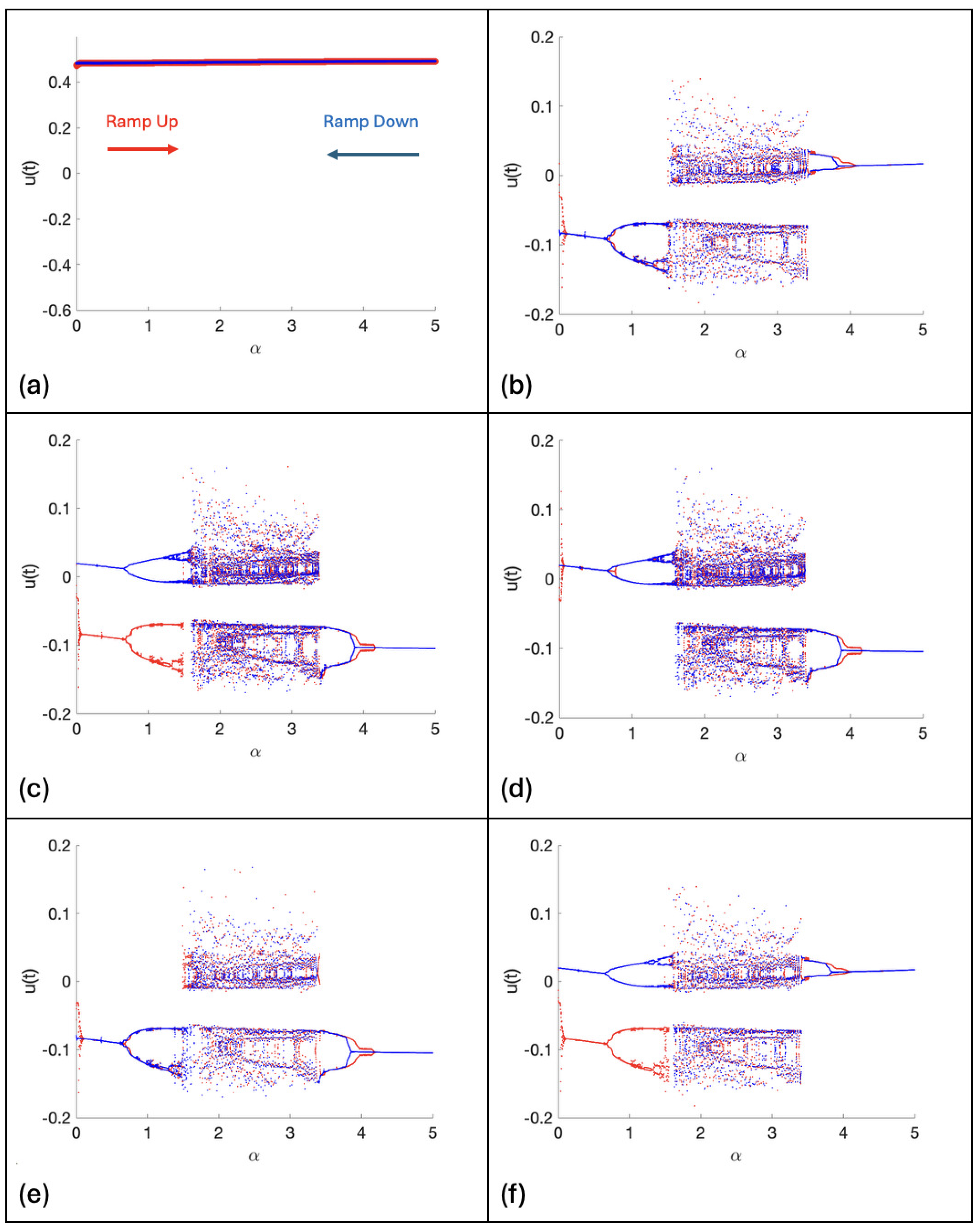
| % Bifurcation Diagram using the Second, Iterative Method with Feedback. |
| clear |
| figure |
| global alpha; |
| xmin=0;xmax=5; |
| ymin=-0.2;ymax=0.2; |
| % Parameters. |
| Max=10000;step=0.0005;interval=Max*step; |
| u=0.1;s=1; % Initial conditions. |
| % Ramp alpha up. Take 2pi time intervals. |
| for n=1:Max |
| alpha=step*n; |
| [t,x]=ode45(’Sys1’,0:2*pi,[u,s]); |
| u=x(2,1); |
| s=x(2,2); |
| rup(n)=x(2,1); |
| end |
| % Ramp alpha down. Take 2pi time intervals. |
| for n=1:Max |
| alpha=interval-step*n; |
| [t,x]=ode45(’Sys1’,0:2*pi,[u,s]); |
| u=x(2,1); |
| s=x(2,2); |
| rdown(n)=x(2,1); |
| end |
| % Plot the bifurcation diagram. |
| hold on; |
| rr=step:step:interval; |
| plot(rr,rup,’r.’,’MarkerSize’,1); % Ramp up, red dots. |
| plot(interval-rr,rdown,’b.’,’MarkerSize’,1); % Ramp down, blue dots. |
| hold off; |
| fsize=20; |
| set(gca,’FontSize’,fsize); |
| axis([xmin xmax ymin ymax]); |
| xlabel(’\alpha’); |
| ylabel(’u(t)’); |
| % Activation function. |
| function [y] = f1(x) |
| y = 3*x*exp(-x^2/2); |
| end |
| % Single Neuron System. |
| function xdot=Sys1(t,x) |
| q=5;p=5;epsilon=0.2;w=2*pi; |
| global alpha; |
| xdot(1)=-x(1)+f1(q*x(2))*f1(p*x(1))+epsilon*sin(w*t); |
| xdot(2)=-alpha*x(2)+alpha*f1(p*x(1))*f1(p*x(1)); |
| xdot=[xdot(1);xdot(2)]; |
| end |
| % End of Program. |
Appendix C
| # Python Program. |
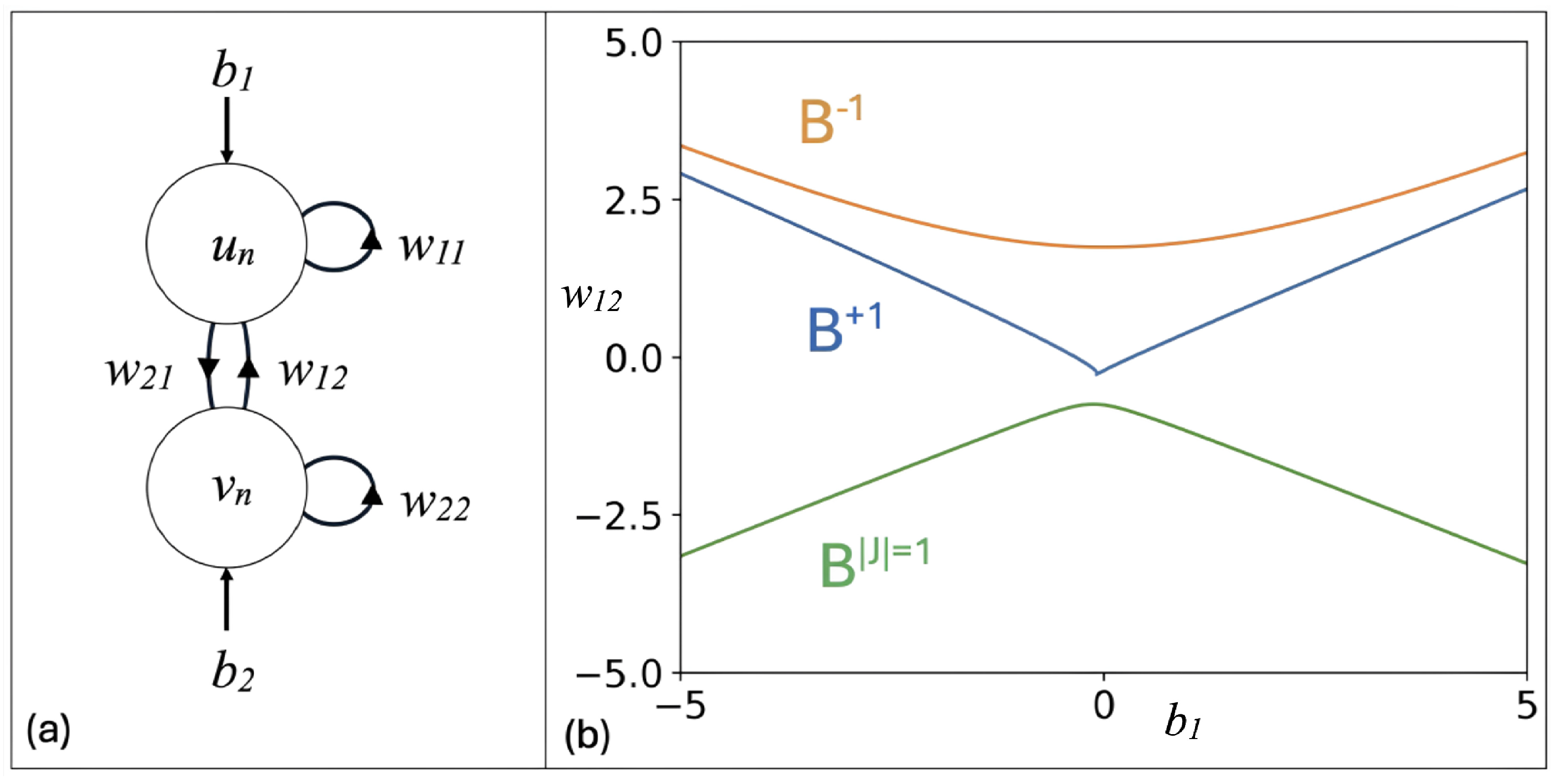
| # Stability diagram. See Figure 6b. |
| import numpy as np |
| import matplotlib.pyplot as plt |
| b2 , w11 , w21 , a , b = -1 , 1.5 , 5 , 0.3 , 0.1 |
| x = np.linspace(-2.5 , 3.2 , 1000) |
| y = b2 + w21 * 3 * (a * x) * np.exp(-a**2*x**2/2) |
| plt.axis([-5 , 5 , -5 , 5 ]) |
| w12 = (1 - w11 *(3 * a * np.exp(-a**2*x**2/2) - 3 * a**3 * x**2 * \ |
| np.exp(-a**2*x**2/2))) / (w21*(3*a*np.exp(-a**2*x**2/2)- \ |
| 3*a**3*x**2*np.exp(-a**2*x**2/2))*(3*b*np.exp(-b**2*y**2/2) \ |
| -3*b**3*y**2*np.exp(-b**2*y**2/2))) |
| b1 = x - w11*(3*(a*x)*np.exp(-a**2*x**2/2)) - \ |
| w12*(3*b*y*np.exp(-b**2*y**2/2)) |
| plt.plot(b1 , w12) |
| plt.xlabel("$b_1$") |
| plt.ylabel("$w_{12}$") |
| plt.rcParams["font.size"] = 30 |
| w12 = (1 + w11 *(3 * a * np.exp(-a**2*x**2/2) - 3 * a**3 * x**2 * \ |
| np.exp(-a**2*x**2/2))) / (w21*(3*a*np.exp(-a**2*x**2/2) - \ |
| 3*a**3*x**2*np.exp(-a**2*x**2/2))*(3*b*np.exp(-b**2*y**2/2) - \ |
| 3*b**3*y**2*np.exp(-b**2*y**2/2))) |
| b1 = x - w11*(3*(a*x)*np.exp(-a**2*x**2/2)) - \ |
| w12*(3*b*y*np.exp(-b**2*y**2/2)) |
| plt.plot(b1 , w12) |
| w12 = - 1 / (w21*(3*a*np.exp(-a**2*x**2/2) - \ |
| 3*a**3*x**2*np.exp(-a**2*x**2/2)) * \ |
| (3*b*np.exp(-b**2*y**2/2)-3*b**3*y**2*np.exp(-b**2*y**2/2))) |
| b1 = x - w11*(3*(a*x)*np.exp(-a**2*x**2/2)) - \ |
| w12*(3*b*y*np.exp(-b**2*y**2/2)) |
| plt.plot(b1 , w12) |
| plt.savefig("stability.png" , dpi = 400) |
| plt.show() |
Appendix D
| # Python Program. |
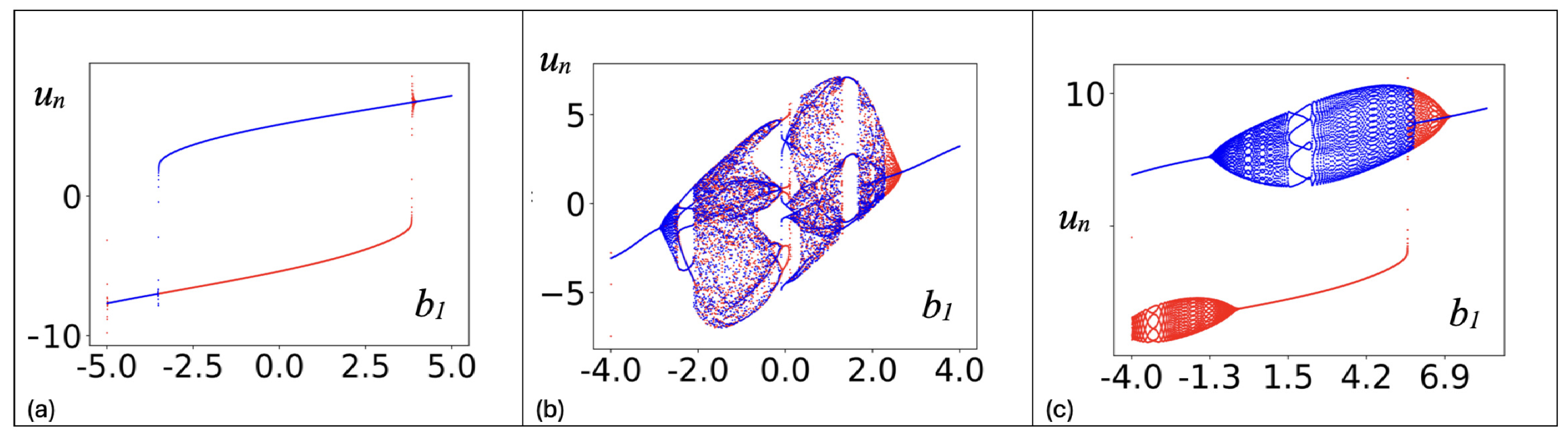
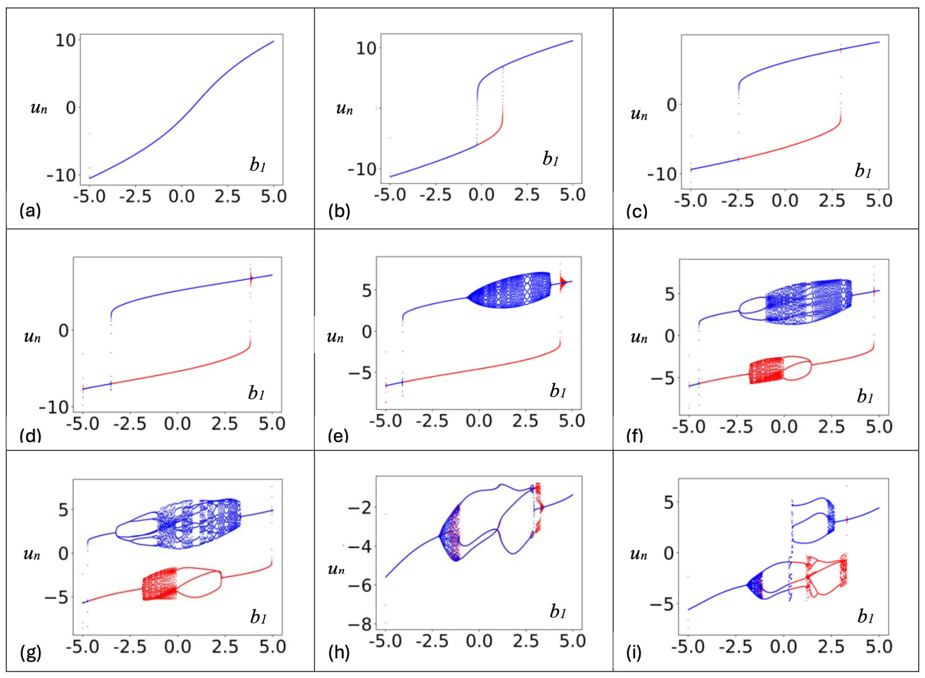
| # See Figure 7b. |
| # Bifurcation Diagrams for a Two-Neuron Module with Adaptive Synapses. |
| # Unstable. |
| from matplotlib import pyplot as plt |
| import numpy as np |
| w12 = -2 |
| b2 , w11 , w21 , a , b = -1 , 1.5 , 5 , 0.3 , 0.1 |
| start, max = -4, 8 |
| half_N = 9999 |
| N = 2 * half_N + 1 |
| N1 = 1 + half_N |
| xs_up, xs_down = [], [] |
| x0, y0 = -7.5, 5 |
| ns_up = np.arange(half_N) |
| ns_down = np.arange(N1, N) |
| def f(x): |
| return 3 * x * np.exp(-x**2 / 2) |
| # Ramp b1 up |
| for n in ns_up: |
| b1 = start + n*max / half_N |
| x = b1 + w11 * f(a * x0) + w12 * f(b * y0) |
| y = b2 + w21 * f(a * x0) |
| xn = x |
| x0 , y0 = x , y |
| xs_up.append([n, xn]) |
| xs_up = np.array(xs_up) |
| # Ramp b1 down |
| for n in ns_down: |
| b1 = start + 2*max - n*max / half_N |
| x = b1 + w11 * f(a * x0) + w12 * f(b * y0) |
| y = b2 + w21 * f(a * x0) |
| xn = x |
| x0 , y0 = x , y |
| xs_down.append([N-n, xn]) |
| xs_down = np.array(xs_down) |
| fig, ax = plt.subplots() |
| xtick_labels = np.linspace(start, max, 7) |
| ax.set_xticks([(-start + x) / max * N1 for x in xtick_labels]) |
| ax.set_xticklabels(["{:.1f}".format(xtick) for xtick in xtick_labels]) |
| plt.rcParams["font.size"] = 30 |
| plt.plot(xs_up[:, 0], xs_up[:, 1], "r.", markersize=1) |
| plt.plot(xs_down[:, 0], xs_down[:,1], "b.", markersize=1) |
| plt.xlabel(r"$b_1$") |
| plt.ylabel(r"$u_n$") |
| plt.show() |
References
- Dong, D.W.; Hopfield, J.J. Dynamic properties of neural networks with adapting synapses. Netw. Comput. Neural Syst. 1992, 3, 267–283. [Google Scholar] [CrossRef]
- Abbott, L.R.; Nelson, S.B. Synaptic plasticity: Taming the beast. Nat. Neurosci. 2000, 3, 1178–1183. [Google Scholar] [CrossRef] [PubMed]
- Tresca, H.E. Mémoire sur l’écoulement des corps solides. Mémoire Présentés par Divers Savants Acad. Sci. Paris 1872, 20, 75–135. [Google Scholar]
- Ewing, J.W. Experimental researches in magnetism. Trans. R. Soc. Lond. 1885, 176, 523640. [Google Scholar]
- Lynch, S. Python for Scientific Computing and Artificial Intelligence; CRC Press: Boca Raton, FL, USA, 2023. [Google Scholar]
- Noori, H.R. Hysteresis Phenomena in Biology; Springer: New York, NY, USA, 2014. [Google Scholar]
- Albesa-González, A.; Froc, M.; Williamson, O.; van Rossum, M.C.W. Weight dependence in BCM leads to adjustable synaptic competition. J. Comput. Neurosci. 2022, 50, 431–444. [Google Scholar] [CrossRef] [PubMed]
- Hu, S.M.; Liu, J.X.; Yao, L.Y.; Song, H.J.; Zhong, X.L.; Wang, J.B. Enlarging the frequency threshold range of Bienenstock-Cooper-Munro rules in WOx-based memristive synapses by Al doping. J. Mater. Chem. C 2025, 13, 3311–3319. [Google Scholar] [CrossRef]
- Wen, W.; Turrigiano, G.G. Developmental Regulation of Homeostatic Plasticity in Mouse Primary Visual Cortex. J. Neurosci. 2021, 41, 9891–9905. [Google Scholar] [CrossRef] [PubMed]
- Yee, A.X.; Hsu, Y.T.; Chen, L. A metaplasticity view of the interaction between homeostatic and Hebbian plasticity. Philos. Trans. R. Soc. B Biol. Sci. 2017, 372, 1715. [Google Scholar] [CrossRef] [PubMed]
- Schmidt, A.; Meindl, T.; Albu-Schäffer, A.; Franklin, D.W.; Stratmann, P. Influence of serotonin on the long-term muscle contraction of the Kohnstamm phenomenon. Sci. Rep. 2025, 15, 16588. [Google Scholar] [CrossRef] [PubMed]
- Ben-Ari, Y.; Danchin, É.É. Limitations of genomics to predict and treat autism: A disorder born in the womb. J. Med. Genet. 2025, 62, 303–310. [Google Scholar] [CrossRef] [PubMed]
- Briones, T.L.; Suh, E.; Jozsa, L.; Rogozinska, M.; Woods, J.; Wadowska, M. Changes in number of synapses and mitochondria in pre-synaptic terminals in the dentate gyrus following cerebral ischemia and rehabilitation training. Brain Res. 2005, 1033, 51–57. [Google Scholar] [CrossRef] [PubMed]
- Briones, T.L.; Suh, E.; Jozsa, L.; Hattar, H.; Chai, J.; Wadowska, M. Behaviorally-induced ultrastructural plasticity in the hippocampal region after cerebral ischemia. Brain Res. 2004, 997, 137–146. [Google Scholar] [CrossRef] [PubMed]
- Liu, Y.Z.; Zhao, J.Y.; Xiao, Y.; Chen, P.; Chen, H.S.; He, E.H.; Lin, P.; Pan, G. Variation-resilient spike-timing-dependent plasticity in memristors using bursting neuron circuit. Neuromorphic Comput. Eng. 2025, 5, 024013. [Google Scholar] [CrossRef]
- Lee, S.H. Plasticity and Memory Retention in ZnO-CNT Nanocomposite Optoelectronic Synaptic Devices. Materials 2025, 18, 2293. [Google Scholar] [CrossRef] [PubMed]
- Provata, A.; Almirantis, Y.; Li, W.T. Multistable Synaptic Plasticity Induces Memory Effects and Cohabitation of Chimera and Bump States in Leaky Integrate-and-Fire Networks. Entropy 2025, 27, 257. [Google Scholar] [CrossRef] [PubMed]
- Bao, B.; Zhu, Y.X.; Ma, J.; Bao, H.; Wu, H.G.; Chen, M. Memristive neuron model with an adapting synapse and its hardware implementations. Sci. China Technol. Sci. 2021, 64, 1107–1117. [Google Scholar] [CrossRef]
- Seralan, V.; Chandrasekhar, D.; Pakiriswamy, S.; Rajagopal, K. Collective behavior of an adapting synapse-based neuronal network with memristive effect and randomness. Cogn. Neurodyn. 2024, 18, 4071–4087. [Google Scholar] [CrossRef] [PubMed]
- Ma, T.; Al-Barakati, A.A.; Jahanshahi, H.; Miao, M. Hidden dynamics of memristor-coupled neurons with multi-stability and multi-transient hyperchaotic behavior. Phys. Scr. 2023, 98, 105202. [Google Scholar] [CrossRef]
- Lynch, S. Dynamical Systems with Applications Using Maple, 2nd ed.; Springer International Publishing: New York, NY, USA, 2010. [Google Scholar]
- Lynch, S. Dynamical Systems with Applications Using Mathematica, 2nd ed.; Springer International Publishing: New York, NY, USA, 2017. [Google Scholar]
- Lynch, S. Dynamical Systems with Applications Using MATLAB, 3rd ed.; Springer International Publishing: New York, NY, USA, 2025. [Google Scholar]
- Lynch, S. Dynamical Systems with Applications Using Python; Springer International Publishing: New York, NY, USA, 2018. [Google Scholar]
- Li, C.; Chen, G. Coexisting chaotic attractors in a single neuron model with adapting feedback synapse. Chaos Solitons Fractals 2005, 23, 1599–1604. [Google Scholar] [CrossRef]

Disclaimer/Publisher’s Note: The statements, opinions and data contained in all publications are solely those of the individual author(s) and contributor(s) and not of MDPI and/or the editor(s). MDPI and/or the editor(s) disclaim responsibility for any injury to people or property resulting from any ideas, methods, instructions or products referred to in the content. |
© 2025 by the authors. Licensee MDPI, Basel, Switzerland. This article is an open access article distributed under the terms and conditions of the Creative Commons Attribution (CC BY) license (https://creativecommons.org/licenses/by/4.0/).
Share and Cite
Lynch, S.T.; Lynch, S. Hysteresis in Neuron Models with Adapting Feedback Synapses. AppliedMath 2025, 5, 70. https://doi.org/10.3390/appliedmath5020070
Lynch ST, Lynch S. Hysteresis in Neuron Models with Adapting Feedback Synapses. AppliedMath. 2025; 5(2):70. https://doi.org/10.3390/appliedmath5020070
Chicago/Turabian StyleLynch, Sebastian Thomas, and Stephen Lynch. 2025. "Hysteresis in Neuron Models with Adapting Feedback Synapses" AppliedMath 5, no. 2: 70. https://doi.org/10.3390/appliedmath5020070
APA StyleLynch, S. T., & Lynch, S. (2025). Hysteresis in Neuron Models with Adapting Feedback Synapses. AppliedMath, 5(2), 70. https://doi.org/10.3390/appliedmath5020070