Article

The Sequential Hotelling Game with One Parameterized Location

Complex Systems Group, Universidad Politécnica de Madrid, C.Universitaria, 28040 Madrid, Spain
*
Author to whom correspondence should be addressed.
AppliedMath 2025, 5(2), 69; https://doi.org/10.3390/appliedmath5020069
Submission received: 9 April 2025 / Revised: 12 May 2025 / Accepted: 22 May 2025 / Published: 13 June 2025

Abstract

:
This article studies the location–price Hotelling game. Numerous studies have been conducted on the Hotelling game with simultaneous decisions; however, in real-life scenarios, decisions are frequently sequential. Unfortunately, studies on the sequential Hotelling (SHOT) game are quite scarce. This article contributes to the study of the SHOT game by considering the case in which the location of one of the players, either the leader or the follower, is externally fixed. The game is studied analytically and by numerical simulation to address scenarios where mathematical analysis is cumbersome due to the discontinuous nature of the game. Simulation is found to be particularly useful in evaluating the subgame perfect equilibrium (SPE) solution of these SHOT games, where the follower outperforms the leader as a very general rule, with very few exceptions. This article complements a previous study of the SHOT game where the two locations are parameterized and paves the way to address the analysis of more sophisticated formulations of the SHOT game, such as those with reservation cost and with elastic demand.

1. Introduction

The spatial competition model defined by H. Hotelling in [1] involves two vendors located on a line selling an identical product with customers equally spread along this line. These firms compete on location and price in the proposed homogeneous market, so that a customer decides to buy the product of a firm depending on the price and the transportation cost to the point of sale, assumed to be linear with the distance in the initial model. The sum of the price of the product and the transportation cost associated with a customer represents the costs associated with purchasing the product by this customer. He established what is known as the principle of minimum differentiation, which means that firms make product that tends to be more equal or, as Hotelling said in his article: “an undue tendency for competitors to imitate each other in quality of goods, location, and in other essential ways”. In the concrete case of Hotelling’s initial model, it implies that companies tend to select similar locations for their stores. Subsequently, a large body of literature on spatial competition and product differentiation emerged, inspiring the development of spatial models of political competition and becoming an indispensable part of economics teaching [2].
Although the Hotelling game caused great criticism due to its limitations, it could not be proven that the principle of minimum differentiation is invalid until fifty years later in [3], where it was proven that a Nash equilibrium (NE) does not exist when the players are too close, which was not noticed in the seminal analysis by Hotelling [1]. In order to circumvent this problem of the nonexistence of NE, the quadratic instead of linear transportation cost was introduced in [3], although some authors are reluctant to adopt this variant of the game, facing its relevance and/or validity [4].
In the usual approach to the Hotelling game, both players decide simultaneously. In contrast to this, the aim of this article is the study of the behavior of the game when the players decide in a leader–follower sequential manner and the location of one of the players, either the leader or the follower, is externally fixed.
The sequential approach to the Hotelling game has been very little studied. This article contributes to its study in the conventional formulation of the game from a simulation-based perspective. This approach can be applied to more sophisticated formulations of the Hotelling game and to other continuous games with discontinuities in their payoff functions.
Section 2 introduces the Hotelling game both with simultaneous choices and with sequential choices (SHOT game in Section 2). The numerical simulation technique implemented in this article is introduced in Section 3. The SHOT game with linear transportation cost is simulated in Section 4, and the SHOT game with quadratic transportation cost (SHOT2) is simulated in Section 5.

2. The Hotelling Game

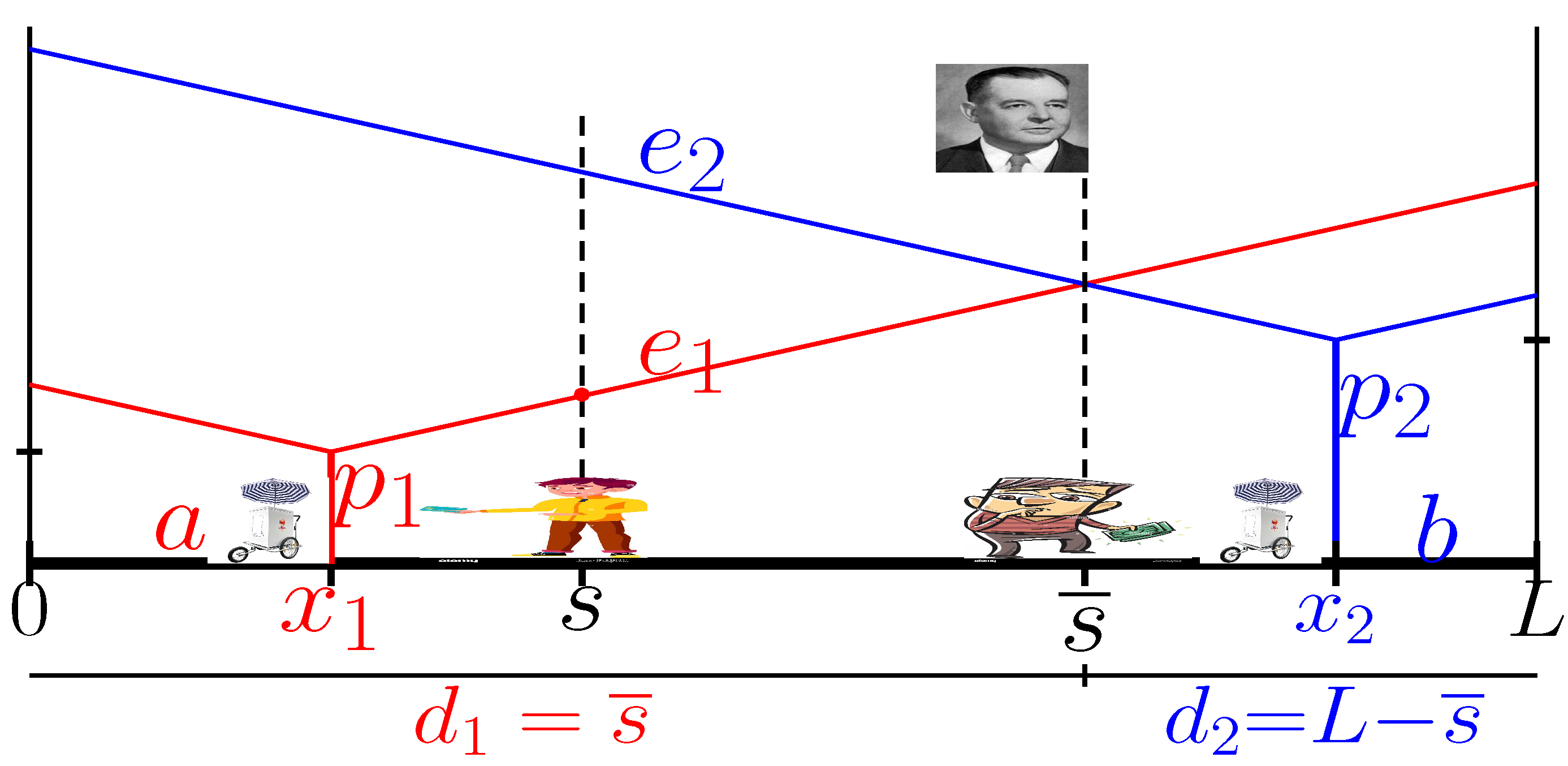
In the Hotelling (HOT) game introduced in the seminal article [1], two players (1 and 2) are located in a line of length L at locations x 1 = a L / 2 and x 2 = L b L / 2 . They sell a homogeneous product at prices p 1 and p 2 to consumers uniformly distributed throughout the line. If the transportation cost is linear with respect to the distance to the player, the expenses (or full prices) of a generic consumer located at s are as follows: e i ( s ) = p i + t | s x i | , i = 1 , 2  . As a result, the indifferent consumer, where e 1 ( s ) = e 2 ( s ) , is located at s ¯ = 1 2 s x + p 2 p 1 t , s x = x 1 + x 2 = L + k ; k = a b , so that the demands to both players are d 1 = s ¯ , d 2 = L s ¯ .
The HOT game is sketched in Figure 1, where the players are presented as “ice cream dealers” [4]. In the figure, two consumers have been identified: one who buys from player 1, and the indifferent one, maybe the young Hotelling (inset).
The payoff functions ( u ) in the HOT game are given in Equation (1), which also take into account the capture of the entire market by a player who charges a very low price, namely, that undercuts the other player. Note that there are two discontinuities in the u -formulas of Equation (1)  (e.g., Figure 6b,c). The existence of such discontinuities is at the origin of the difficulties that arise in the study of the HOT game.
u 1 = L p 1 if p 1 < p 2 t d x d 1 p 1 if | p 1 p 2 | < t d x 0 if p 1 > p 2 + t d x , u 2 = L p 2 if p 2 < p 1 t d x d 2 p 2 if | p 1 p 2 | < t d x 0 if p 2 > p 1 + t d x d x = x 2 x 1
The Nash equilibrium (NE) in prices in the HOT game with given locations found in [1] is given in Equation (2)1. That is, p 1 is the best response to p 2 and p 2 is the best response to p 1 .
( p 1 , p 2 ) = t 1 3 ( 3 L + k , 3 L k ) ( d 1 , d 2 ) = 1 6 ( 3 L + k , 3 L k )
Because u 1 * = d 1 * p 1 * increases with a and u 2 * = d 2 * p 2 * with b , both players would tend to coincide in their location, a phenomenon that in [1] is referred to as the minimum differentiation principle. However, long after the seminal article by Hotelling, it was proven that an NE only exists under constraints that impede such an unrestricted approach in the player locations in NE [3,5,6,7]. In order to circumvent the serious problem of the nonexistence of an NE, quadratic transportation cost with respect to the distance, i.e., e i ( s ) = p i + t ( s x i ) 2 , i = 1 , 2 was proposed in [3]. The HOT game Quadratic transportation cost is also considered in this study, albeit some authors are reluctant to consider this somehow ad hoc variant of the game. For example, T.Puu stated in [8]: “Further, to escape some consequences of the paradox, the unrealistic and contrived idea of quadratic transportation costs was launched and became popular”.
Note that the HOT game is not studied in a global way, that is, considering simultaneously location and price variables, a scenario in which no NE exists [9]. In contrast to the global approach, the game is analyzed in a two-stage process, first analyzing the effect of the choice of prices with fixed locations and then considering the locations as variable parameters. It is also important to note that in the standard approach to the game, both players decide simultaneously.
There exists an immense body of literature dealing with the original Hotelling game and with its variants that is not reviewed here. However, we refer to the recent overview in [2]. References dealing with sequential moves in the HOT game in particular are quite scarce. Among them, the article by S.Anderson, to which we will refer in this study, stands out. In reference [10], only the linear transportation cost is considered. In contrast to this, most of the not numerous articles dealing with the SHOT game stray to quadratic transportation cost, easier to analyze. This is the case of the reference [11]. By the way, in the HOT review reference [2], sequential HOT is not mentioned, in fact the article [10] does not appear in its bibliography.

The Sequential Hotelling Game

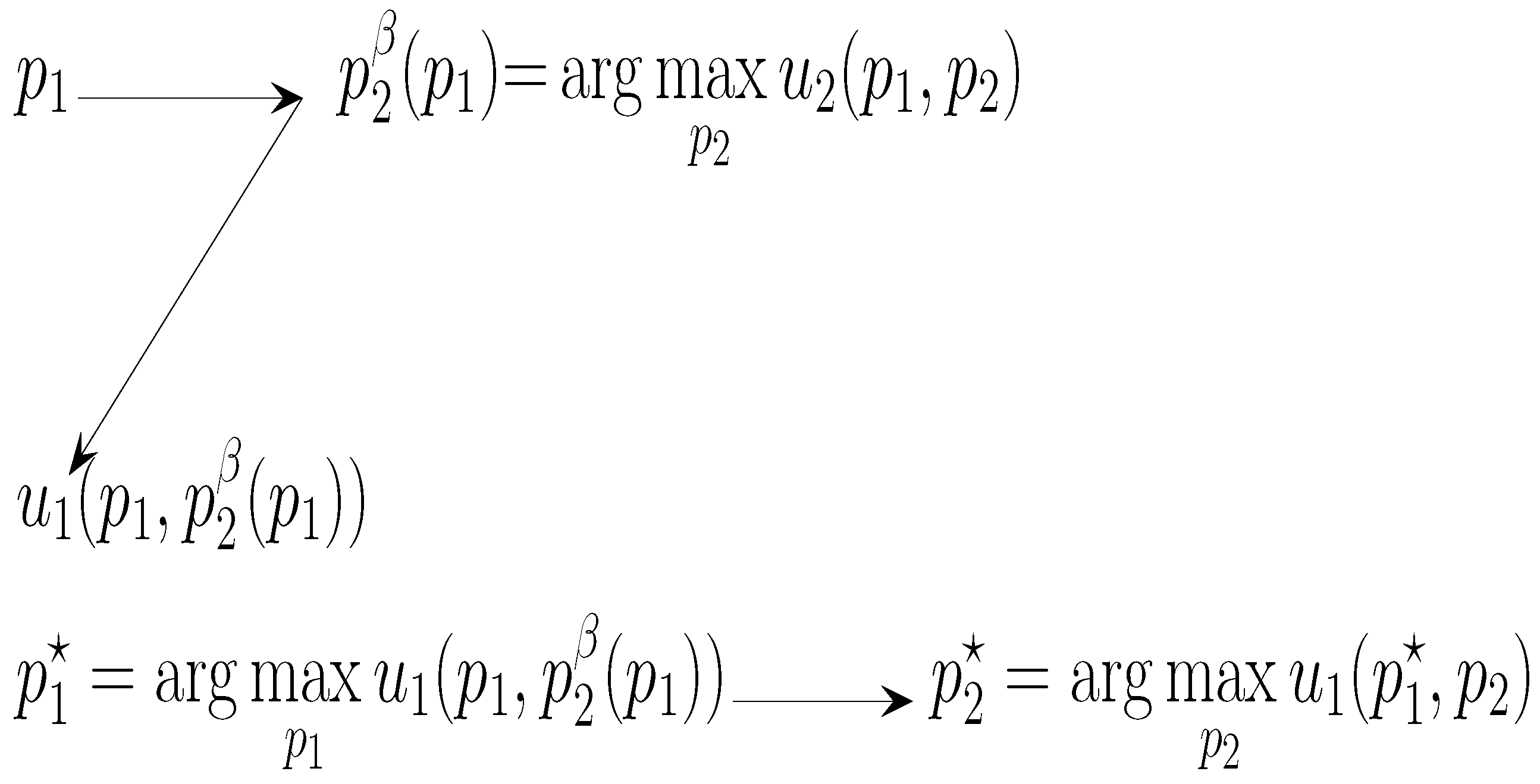
At variance with an implicit assumption in the seminal formulation of the HOT game, in this article the players do not decide simultaneously but sequentially. Thus, one of the players, the leader (or first mover) decides first, then the other player, the follower (or second mover), adopts the best response to the known decision of the leader. The sequential Hotelling game will be referred to as the SHOT game, where according to the backwards induction principle, in the SHOT game the leader assumes that the follower player 2 would react optimally to any choice of player 1. Figure 2 sketches the backwards induction principle in the price variables, where β stands for best response and the -marked prices denote the SPE solution.
In a previous study [12], the two-stage approach (first prices, then locations) was scrutinized in the SHOT game. In this work, an advance is made in the direction of a global approach to the study of the SHOT game by analyzing two complementary SHOT game scenarios: ( i ) the leader decides not only the price but also the location, while the location of the follower is fixed exogenously (scenario referred to as SHOT-b), and ( i i ) the follower decides not only the price but also the location, whereas the location of the leader is fixed exogenously (SHOT-a).
The mathematical analysis of the SHOT game is complicated in general due to the discontinuities in the response functions. This is why we will resort to simulation in a lattice, as explained in the next section. Additionally, the backwards induction principle will be programmed in a direct way (as explained when commenting Figures 13 and 18), although this approach demands very high computational resources.

3. Numerical Simulation

In the numerical simulations in this article, a large number of players of type 1 (leader) and of type 2 (follower) are arranged in a two-dimensional N × N lattice. Every ( i , j ) cell of the lattice is occupied by a player, alternating in site occupation in a chessboard form, so that if 0 ( i + j ) ( mod 2 ) the cell ( i , j ) is occupied by a player 1, and if 1 ( i + j ) ( mod 2 ) the cell ( i , j ) is occupied by a player 2.
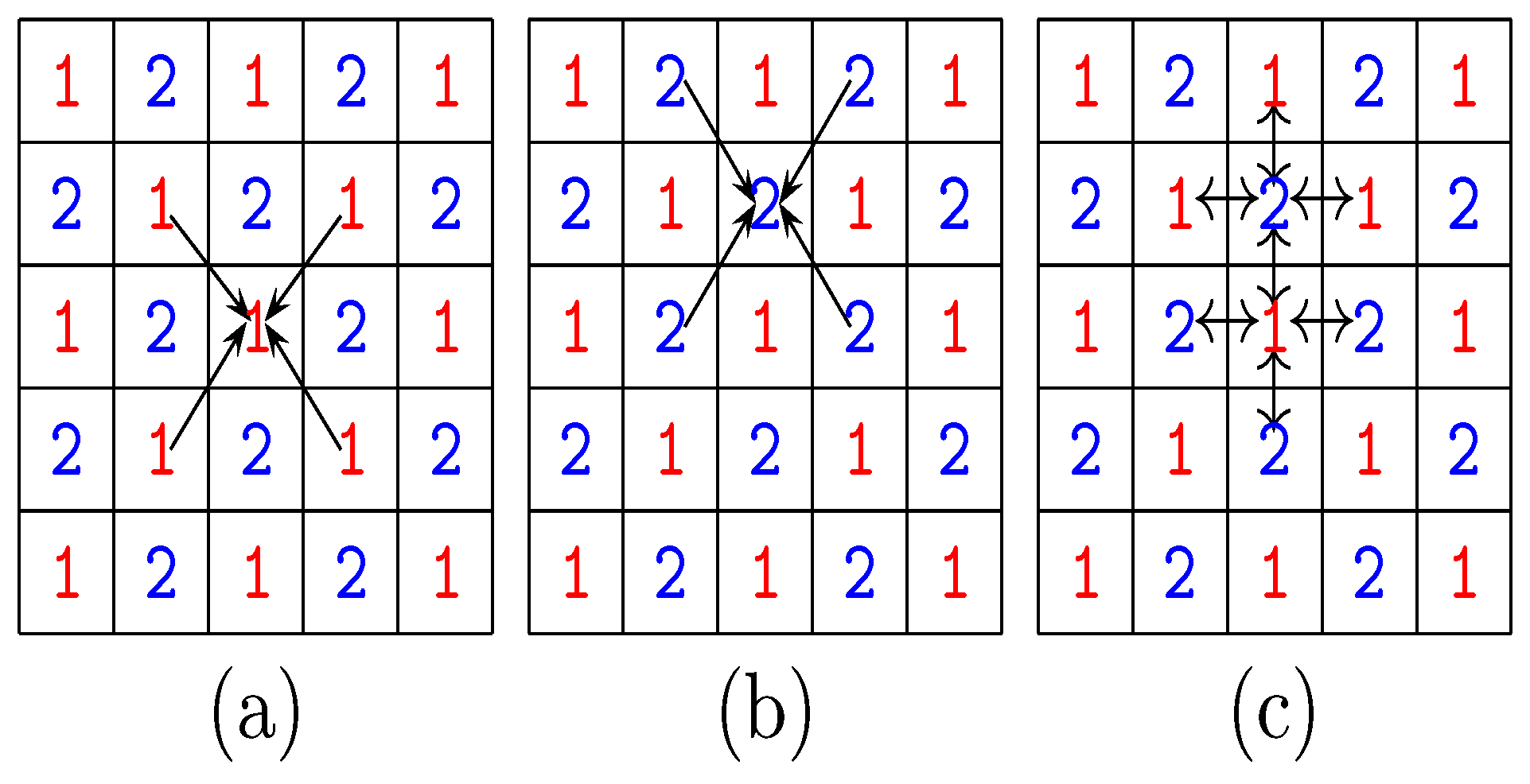
Consequently, every player is surrounded by four partners ( 1 - 2 , 2 - 1 ), and four mates ( 1 - 1 , 2 - 2 ) as Figure 3 illustrates.
The initial prices p are assigned to both types of players at random from a uniform distribution in the [ 0 , p m a x ] interval, where p m a x denotes the maximum available price. Thus, initially it is p ¯ p m a x / 2 and σ p p m a x 2 / 12 for both players. In the SHOT-b game, the initial locations x 1 are assigned to the leader players at random from a uniform distribution in the [ 0 , L / 2 ] interval, while all the player 2 followers in the lattice are assigned to a fixed x 2 location. Therefore, it is initially x 1 ¯ L / 4 in the SHOT-b game. In the SHOT-a game, the initial locations x 2 are assigned to the follower players at random from a uniform distribution in the [ L / 2 , L ] interval, while all the player 1 leaders in the lattice are assigned to a fixed location x 1 . Therefore, it is initially x 2 ¯ 3 L / 4 in the SHOT-a game. In both scenarios, it is initially σ x L 2 / 28 ,
The game is iterated in a cellular automata (CA) manner [13], i.e., with uniform, local, and synchronous interactions. The arrows in the generic players in Figure 3 aim to make clear that the interactions are local, i.e., they involve only nearest-neighbors. Thus, in the updating steps (Figure 3a,b) both types of player scrutinize their NE–NW–SE–SW mate neighbors (Please note that NE stands here for north–east and not Nash equilibrium), whereas playing concerns (Figure 3c) the N–S–E–W partner neighbors.
At every time-step,
  • Every leader player 1 in the lattice will act first and will locate which state variables among that of himself and those of his mate neighbors would provide him the highest payoff applying the backwards induction principle. Such a generic leader will adopt the best local state variables (Figure 3a).
  • After updating the state variables of every player 1 in the lattice, each follower player 2 will locate among that of himself and those of his mate neighbors the state variables that provide the best payoff when playing with his partner neighbors: The generic follower will adopt the best values of the state variables (Figure 3b).
  • Once the moves are made, every player plays with his four adjacent partners such that the payoff u i , j ( T ) of a given individual at time-step T is the average over these four games (Figure 3c).
The simulations performed in this article have been implemented using Fortran code with double precision variables. Table 1 shows the Fortran code that implements the leader update in the SHOT-b game with t = 1 . The HOT subroutine implements the Hotelling game with L r l l , 2 L r 2 L and x 2 x x 2 , whose values are accessible via the common sentence. The subroutine performs the updating of the location and price of the leader in the (i,j) cell site up to x1x and p1p supported in the current values of the locations and prices stored in the WXX and WPP working matrices. The application of the backwards induction principle is supervised in Table 1 because only the three best potential responses to the ( p 1 , a ) choice of the leader, U , M and N given in Equation (3) are scouted. An example of the best response of type M is given in Figures 5–7c and an example of the best response of type U is given in Figures 6 and 7b.
p 2 U ( p 1 , a ) = p 1 t ( L b a + ϵ )
p 2 M ( p 1 , a ) = 1 2 ( p 1 + t ( L a + b ) )
p 2 N ( p 1 , a ) = p 1 + t ( L b a ϵ )
Table 2 shows the Fortran code that implements the update of the follower’s price located in the (i, j) cell up to the p2p price, again in the SHOT-b game with t = 1 .
The Fortran codes that implement the update of the leader and of the follower in the SHOT-a game with t = 1 are given in Table A1 and Table A2 in the Appendix A.
In the simulations of this work, N = 200 and p m a x = 10 . Only the model with t = 1 will be considered, and the length of the market will be fixed to L = 3.0 or to L = 1.0 . In the forthcoming figures, information regarding the leader player 1 will be in red, and the information regarding the follower player 2 will be in blue. A toy example of the initial iteration in the SHOT-b game is given in Figure A1 in the Appendix A.

4. Simulation of the Sequential Hotelling Game

4.1. The SHOT-b Game

4.1.1. Simulation Dynamics

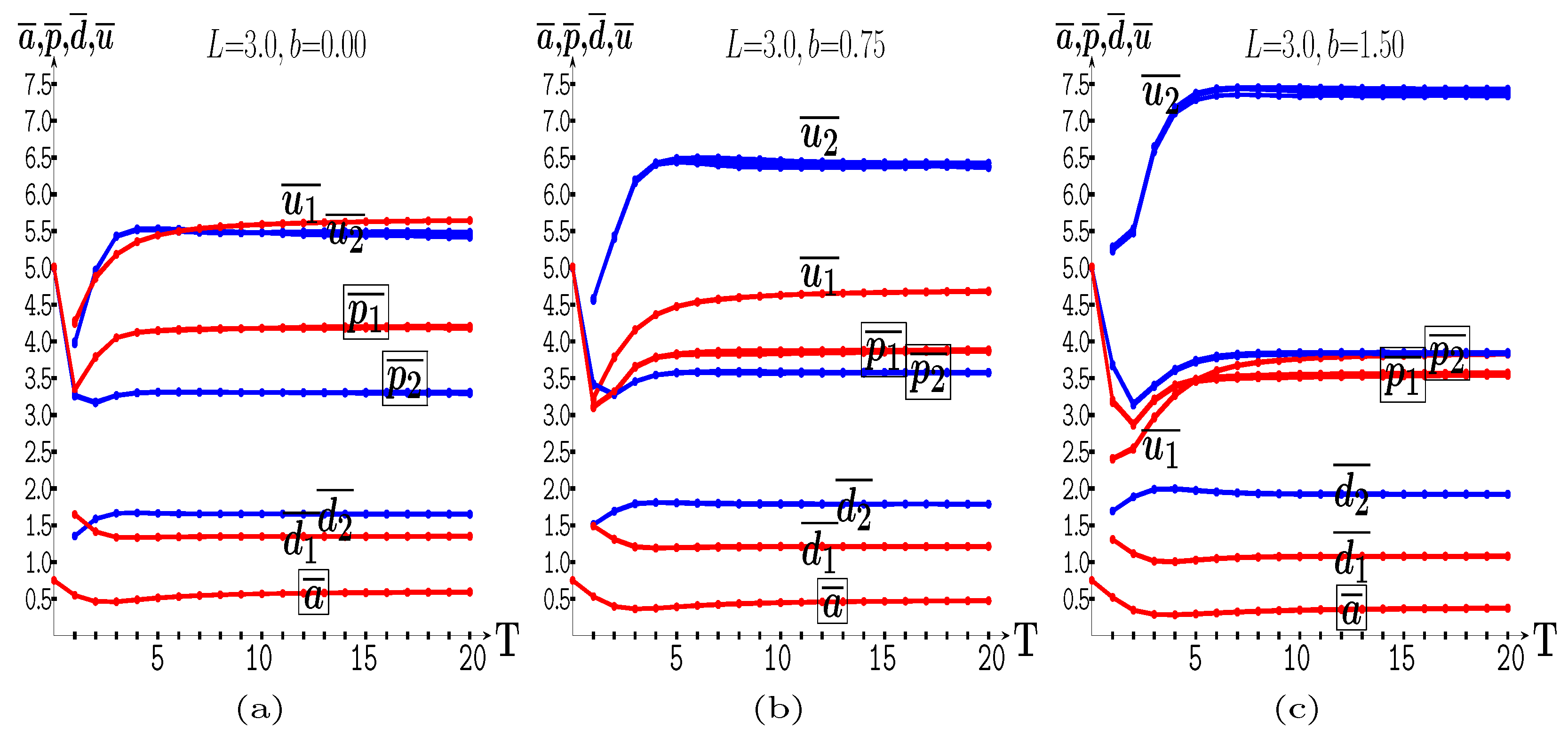
Figure 4 deals with the dynamics in the simulation of the SHOT-b game with three values of b up to T = 20 . In these three scenarios, the averages of the state variables quickly converge to a steady state, so that by T = 20 (or before) the dynamics are virtually stabilized. This is so in the five simulations, i.e., five initial randomizations of prices and location of the follower, reported in the figure, which are almost coincident. In Figure 4a, the follower is located at the right end of the market segment ( b = 0.0 ) uch that the leader exceeds the follower in the steady state, although to a very low extent. In contrast to this, in Figure 4b with the follower located at 3 L / 4 and in Figure 4c where the follower is located in the middle of the market segment ( b = 1.5 ), the follower exceeds the leader in the steady state; this is particularly true in the latter case.
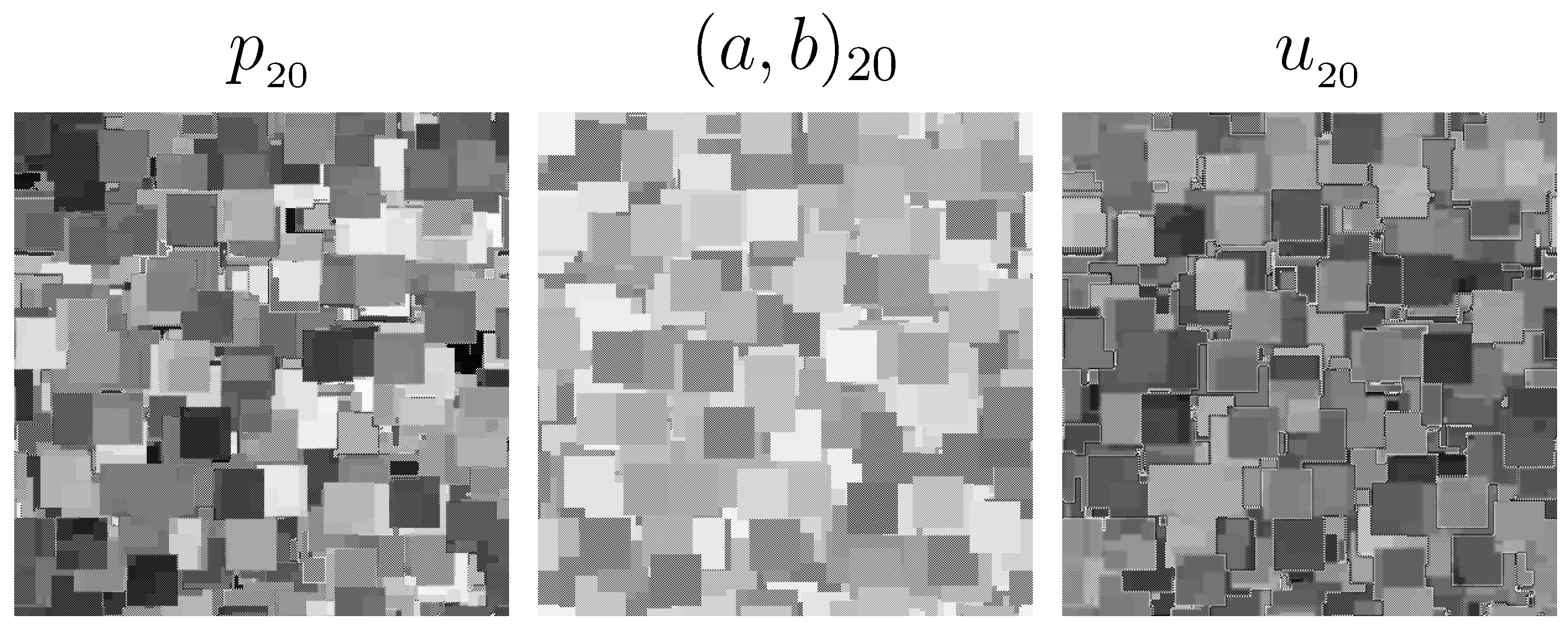
The patterns of p , ( a , b ) and u in one simulation of Figure 4c at T = 20 are given in Figure A2 in the Appendix A.
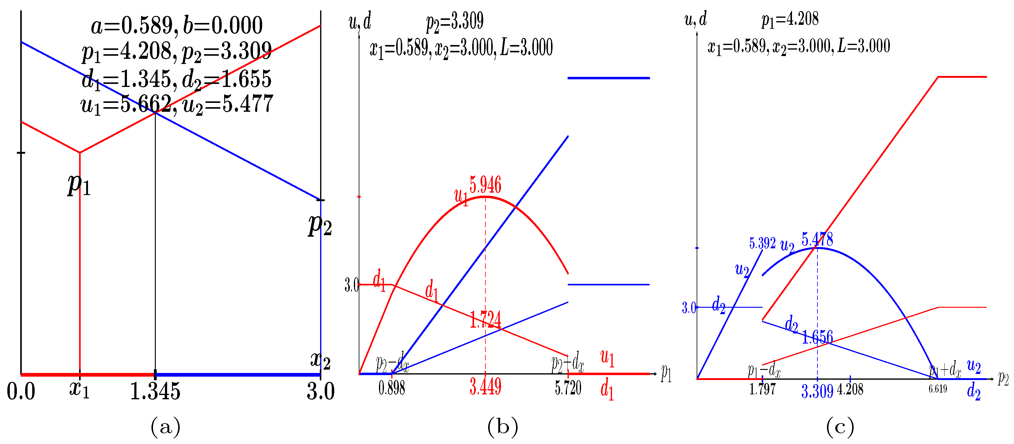
Figure 5, Figure 6 and Figure 7 deal with the games in the steady states of the simulations of Figure 4. The layout of such games are shown in the far-left snapshots of the figures. The payoffs and demands of the games in which the price of one player is parameterized are shown in the central and far-right snapshots. These are obtained by sampling the [ 0 , 1.1 ( p + d x ) ] p -interval in 4000 equidistant points.
In Figure 5, it is k = 0.589 0.000 = 0.589 . In Figure 5b, it is shown that the best response to p 2 = 3.309 is not p 1 = 4.208 but p 1 M ( p 2 = 3.309 ) = 3.449 d 1 = 1.724 u 1 = 5.496 . Figure 5c proves that the best response to p 1 = 4.208 is p 2 M ( p 1 = 4.208 ) = 3.309 = d 2 = 1.665 u 2 = 4.208 · 1.665 = 5.478 .
In Figure 6b, it is shown that the best response to p 2 = 3.584 is not p 1 = 3.889 but p 1 U ( p 2 ) = 1.805 = 3.584 ( 2.250 0.471 ) 0.001 . Figure 6c proves that the best response to p 1 = 3.889 is p 2 M ( p 1 = 3.889 ) = 3.584 d 2 = 1.792 u 2 = 3.889 · 1.792 = 6.424 .
In Figure 7b, it is shown that the best response to p 2 = 3.839 is not p 1 = 3.547 but p 1 M ( p 2 = 3.389 ) = 2.710 = 3.839 ( 1.500 1.129 ) 0.001 . Figure 7c proves that the best response to p 1 = 3.547 is p 2 M ( p 1 = 3.547 ) = 3.838 d 2 = 1.919 u 2 = 3.838 · 1.919 = 7.365 .
The price values were the payoffs of the U and M responses equalize, i.e., u i U ( p ^ j ) = u i M ( p ^ j ) , ( i , j ) = ( 1 , 2 ) , ( 2 , 1 ) , are given in Equation (4)2. Thus, for example, in the scenario of Figure 7c it is p ^ 1 = 9.000 + 0.371 1.500 4 3.0 · 0.371 ) = 3.651 , very close to p 1 = 3.547 . That is why u 2 U = 7.357 is very close to u 2 M = 7.365 .
p ^ 1 = ( 3 L + a b 4 L a ) t , p ^ 2 = ( 3 L a + b 4 L b ) t
No best response is of type N in any the three (c)-scenarios of Figure 5, Figure 6 and Figure 7. This is because the players are not close enough to allow to the N response to emerge as the best solution3.

4.1.2. a -Response Given b and Prices

Figure 8 shows the features of the a -response in the HOT game given the prices achieved in the steady states of the simulations of Figure 4. In the three scenarios of Figure 8, the increase in a , i.e, movement to the center, induces an increase in the payoff of player 1 and a decrease in the payoff of player 24.

4.1.3. Parameterized b

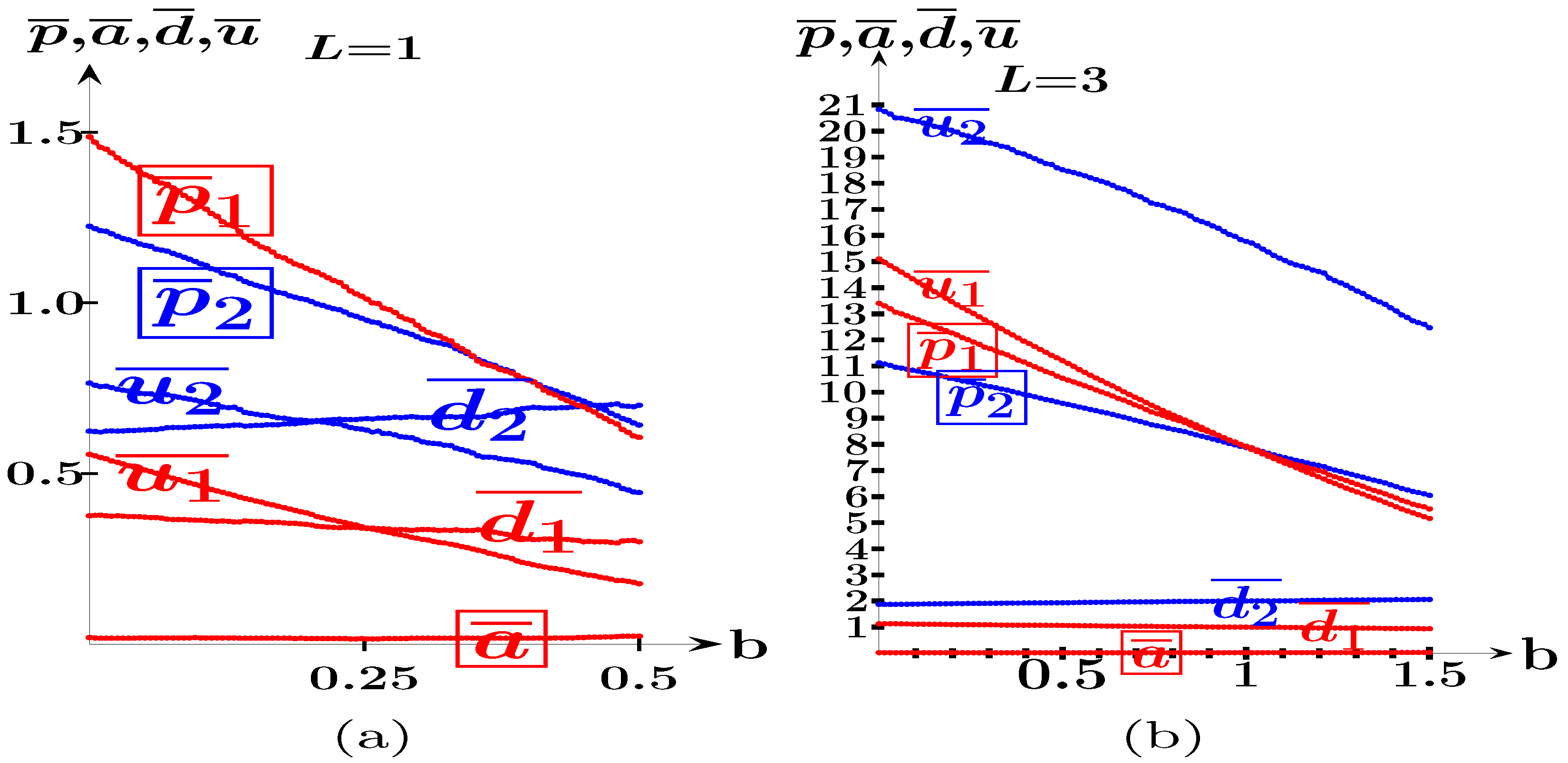
Figure 9 deals with the simulation of the SHOT-b game with variable b . Figure 9a deals with the case of L = 1.0 , whereas Figure 9b deals with the case of L = 3.0 . In both scenarios, ( i ) the leader exceeds the follower only with very low values of b , that is, when the follower is very far away from the market center, and ( i i ) the maximum advantage of the follower is reached at b = L / 2 , that is, when the follower is located at the market center.
The average values of the (location, price) of the leader and that of the follower’s price shown in Figure 9 fit almost perfectly to the values in the SPE solution of the SHOT-b game given in Equation  (5), which induce d 1 = L a  5, so that u 1 = L a 3 L + a b 4 L a t  6.
It is discovered that p 1 = p ^ 1 ( a , b ) and that the price in Equation (5c) is the M -response from b to ( a , p 1 ) , that is, p 2 = p 2 M ( a , p 1 ) . Equation (5) generalize those provided in [10] for L = 1.0 . Incidentally, in the article [14], the L = 1 scenario is also only taken into account with an additional, somehow spurious, variant in the notation: b is the distance to zero, not to one as is customary in the notation of the HOT game.
a = 1 9 23 L + 3 b 8 L ( 7 L + 3 b )
p 1 = 3 L + a b 4 L a t
p 2 = 1 2 p 1 + t ( L a + b )
According to Figure 9, the follower obtains the maximum payoff when he is located in the center of the market segment, in which case,
b # = L 2 , a # = 1 9 49 2 8 17 2 L = 0.1307 L
p 1 # = 5 L 2 + a # 4 L a # t = 1.1846 L t
p 2 # = 1 2 p 1 # + t ( 3 L 2 a # ) = 1.2769 L t
The demands and payoffs associated to the solution in Equation (6) are7,
d 1 # = 0.3615 L , u 1 # = 0.4282 L 2 t
d 2 # = 0.6385 L , u 2 # = 0.8153 L 2 t

4.2. The SHOT-a Game

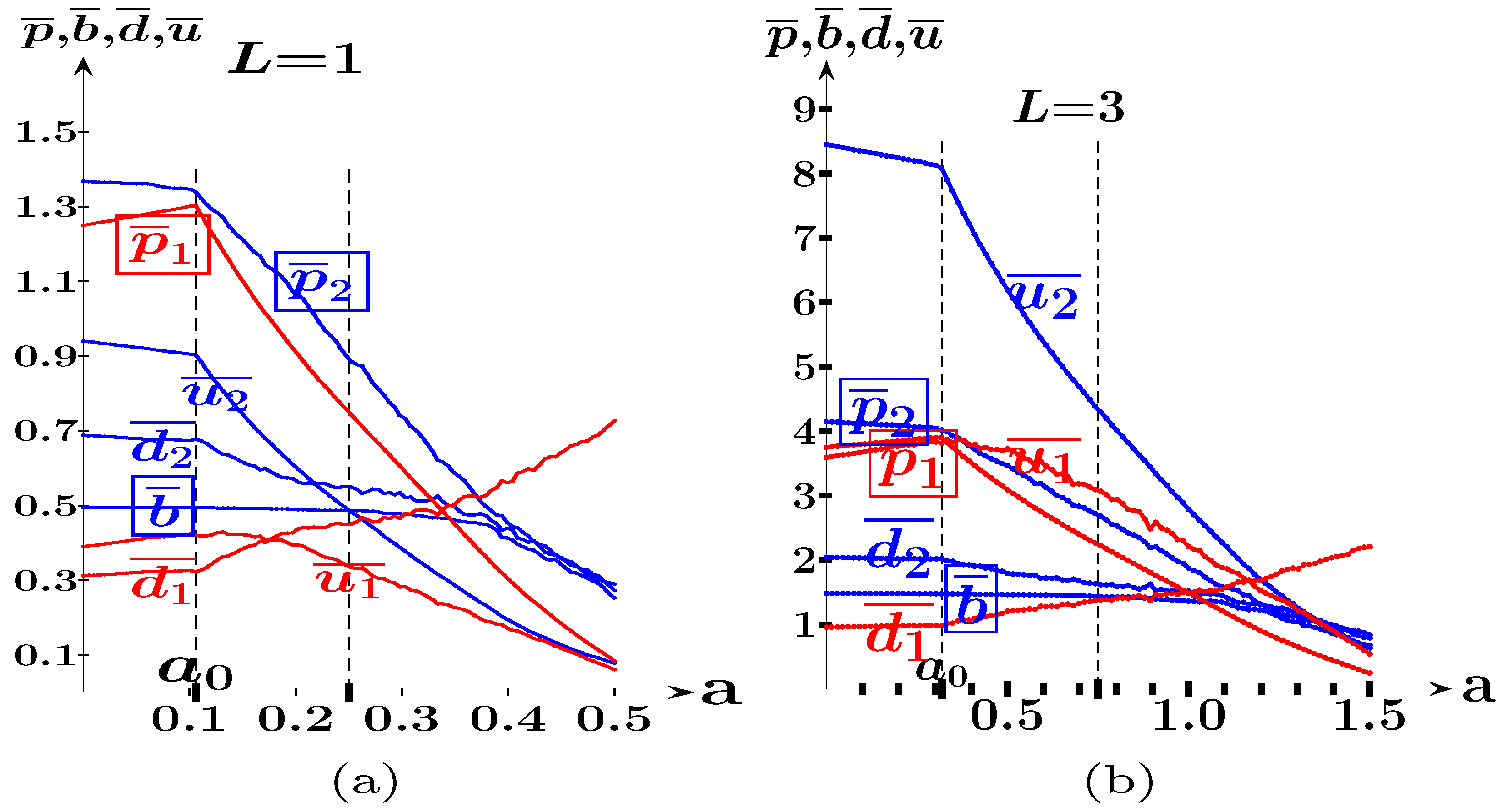
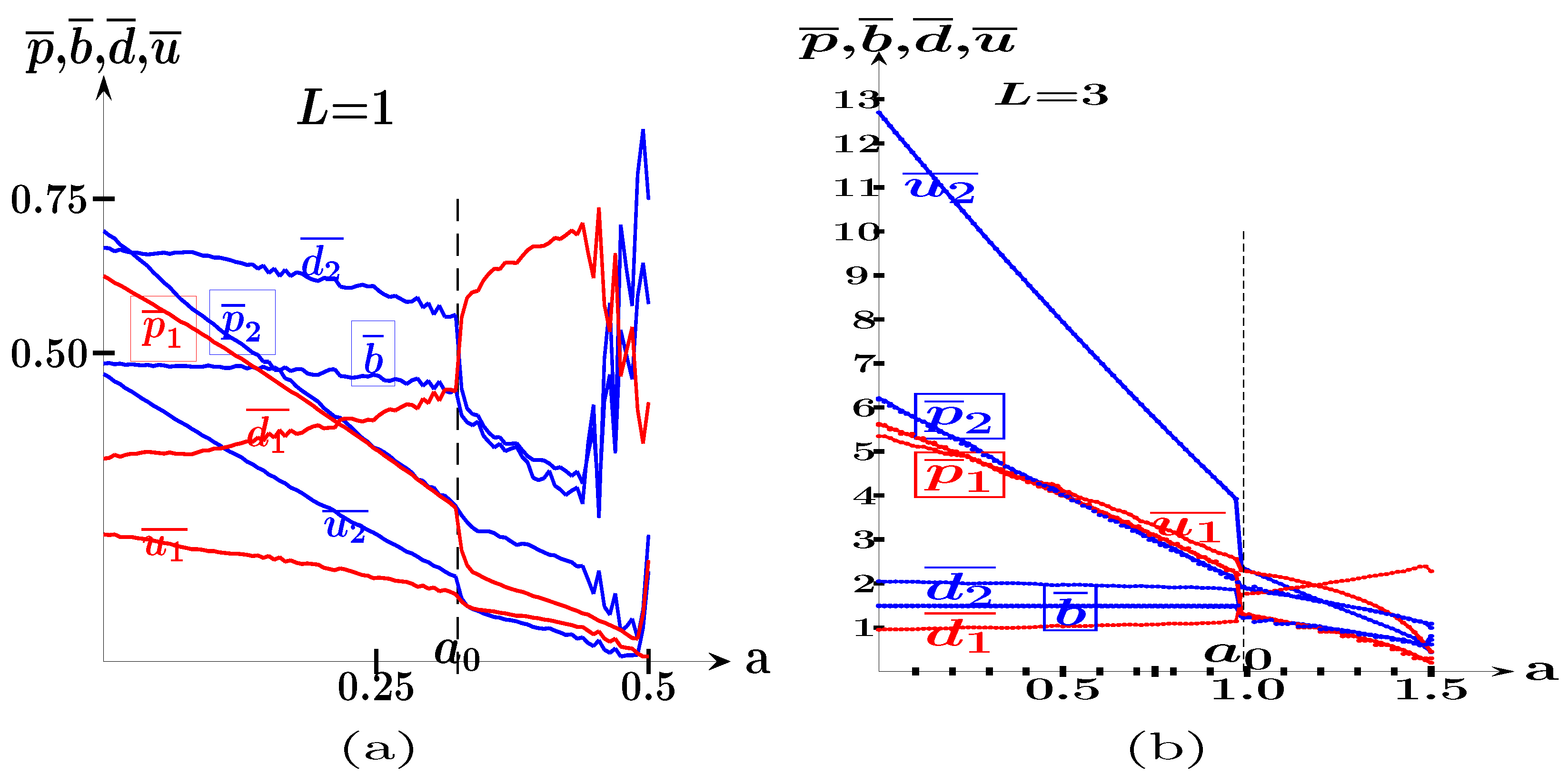
Figure 10 deals with the simulation of the SHOT-a game with variable a . Figure 10a deals with the case of L = 1.0 , whereas Figure 10b deals with the case of L = 3.0 . In both scenarios, ( i ) the follower player 2 exceeds the leader, although the follower advantage decreases with increasing a such that with high a both players obtain a virtually equal payoff, ( i i ) it is b ¯ L / 2 up to a at least L / 4 , that is, the follower is located in the center of the market segment, provided that the leader is not close to the center, and ( i i i ) The aspect of the graphs changes at the critical value a 0 whose value is given in Equation (88. Therefore, in Figure 10a, it is a 0 = 0.106 , and in Figure 10b, it is a 0 = 0.318  .
a 0 = 59 2 24 3 2 L
In the two scenarios of Figure 10, if a < a 0 , the average variables in the simulation fit very well the values in the SPE solution given in Equation  (9a). It is revealed that p 1 = 1 2 3 L + a b t , and that p 2 = p 2 M ( b , p 1 ) = 1 2 p 1 + t ( L a + b ) .
b = 1 2 L , p 1 = 1 2 5 2 L + a t , p 2 = 1 4 11 2 L a t
d 1 = 1 8 5 2 L + a , u 1 = 1 16 5 2 L + a 2 t
d 2 = 1 8 11 2 L a , u 2 = 1 32 11 2 L a 2 t
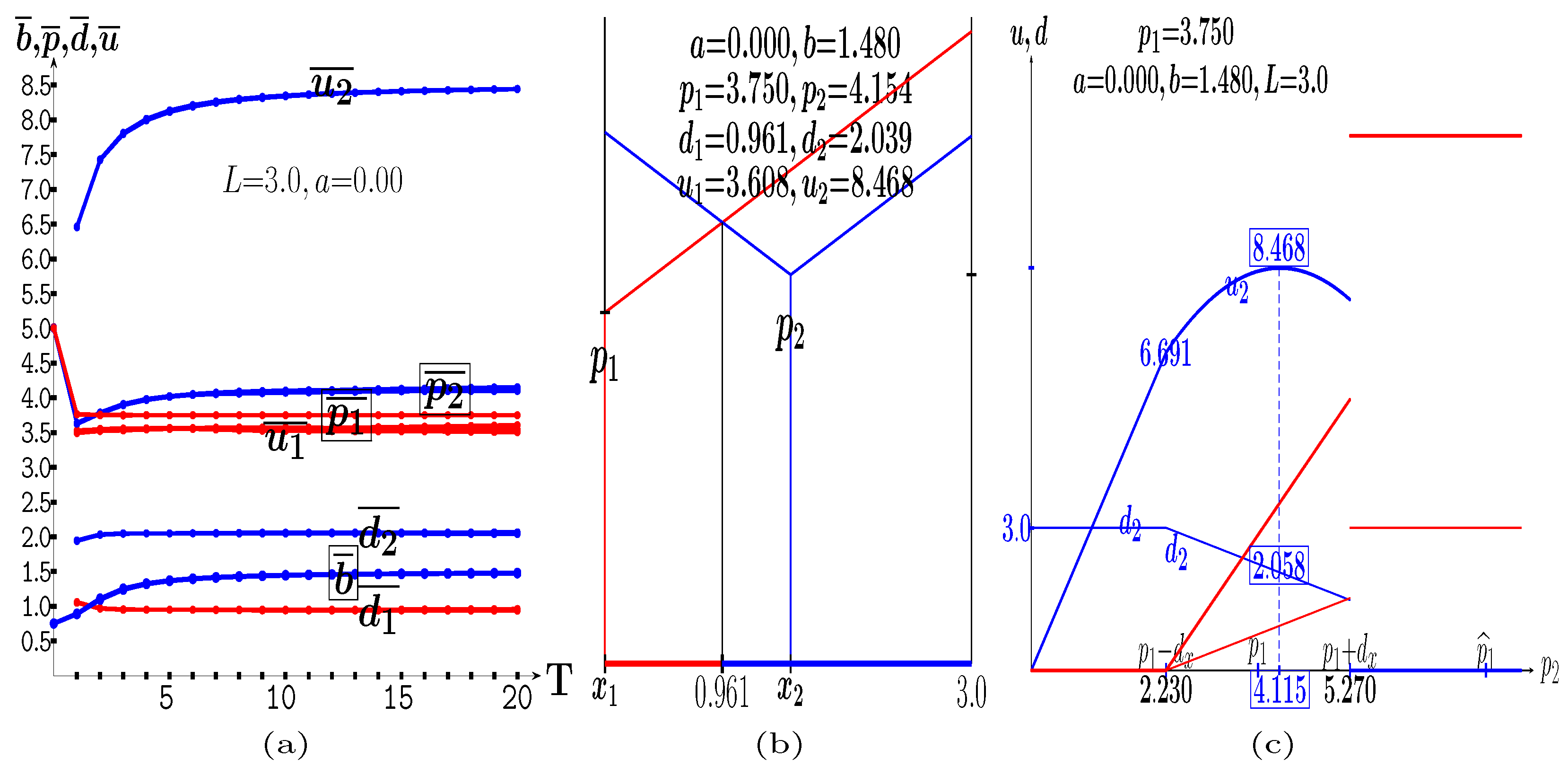
Figure 11 deals with the SHOT-a=0.0 game. Figure 11a shows the dynamics up to T = 20 , where the simulations quickly converge to virtually the same average steady-state variables. The game with the average values at T = 20 of one simulation is shown in Figure 11b. Figure 11c shows the effect of the price response of player 2 in the scenario of the game of Figure 11b. Remarkably, the average value of the player 2 price reached through simulation, p ¯ 2 = 4.154 , is very close to p 2 M = 4.115 . Moreover, u ¯ 2 = u 2 M = 8.468 .
In the [ a 0 , L / 4 ] interval of Figure 10, the average variables in the simulation very well fit the values in the SPE solution given in Equation (10a). It is shown that p 1 = p ^ 1 ( b ) = ( 3 L + a b 4 L a ) t and that p 2 = p 2 M ( p 1 , b ) , as in the [ 0 , a 0 ] interval 9.
b = 1 2 L , p 1 = 5 2 L + a 4 L a t , p 2 = 2 L L a t
d 1 = L a , u 1 = L a 5 2 L + a 4 L a t
d 2 = L L a , u 2 = 2 L L a 2 t
Figure 12 deals with the simulation of the SHOT-a=L/4=0.75 game. Diverging from the scenario in Figure 11, in Figure 12 the average value of the player 2 price reached through simulation, p ¯ 2 = 2.854 , is not so close to p 2 M = 2.993 . In any case, u ¯ 2 = 4.468 is not far from u 2 M = 4.479 . Incidentally, p 2 M = 2.992 is very close to p 2 N = 3.015 in Figure 12c.
The output of the lattice simulation becomes rather unclear with high a . Therefore, we will resort here to the direct implementation of the backwards induction principle. This has been performed by means of the Fortran code in Table A3 in the Appendix A. This code produces the outputs in Figure 13, where player 1 obtains the maximum payoff at the location a # already referred in Equation (6a10. Thus, the pair ( a # , p 1 # ) , ( b # , p 2 # ) whose formulas are given in Equation (6) is the SPE solution in the location–price SHOT game.
The demands in Equation (10) equalize at a = L / 4 ( L a = L L a ). Further increase in a up to a = 3 L / 8 induces the price of the leader in the SPE solution to become of the form p 1 = L + b L b ( L b a ) and the best response of the follower to become of the type N . Therefore, Equation (11) describe the SPE solution when a [ L / 4 , 3 L / 8 ] , where is b = d 1 , 2 = L / 2 . At a = L / 3 , it is p 1 = L / 2 , p 2 = 4 L / 3 , and at a = 3 L / 8 , it is p 1 = 3 L / 8 , p 2 = L / 2 .
b = L 2 , p 1 = 3 L 2 a t , p 2 = 2 L 2 a t
d 1 = L 2 , u 1 = 3 L 2 a L 2 t ; d 2 = L 2 , u 2 = 2 L 2 a L 2 t
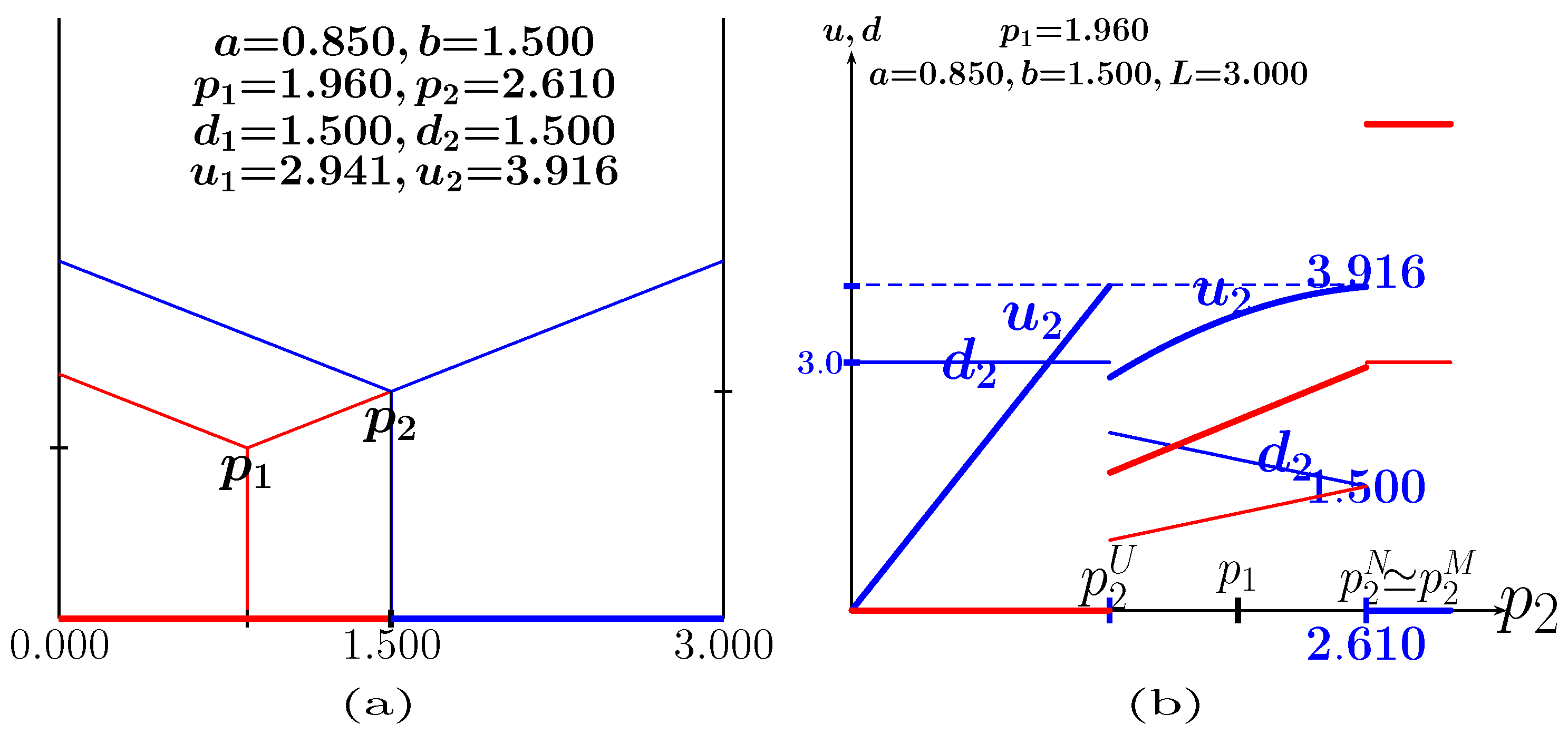
Figure 14 deals with the SHOT-a game at a = 0.85 , L = 3.0 . Figure 14a shows that in the market segment [ L / 2 , L ] the expenses regarding both players are equal such that the players in this segment are in principle indifferent as to which firm (player) to buy from. To overcome this indefiniteness, the Fortran code has been programmed so that consumers in this segment will buy from their closer firm, i.e., player 2.
In the [ 3 L / 8 , L / 2 ] a -interval, b equalizes p 2 , with b = p 2 = 1 2 ( p 1 + L a ) 11. Moreover, d 2 = b = p 2 , with p 1 = 2 b + a L 12, and as a result, Equation (12) describes the SPE solution in the [ 3 L / 8 , L ]   a -interval13.
b = p 2 = ( L 1 2 2 L ( 4 a L ) ) t , p 1 = ( L + a 2 L ( 4 a L ) ) t
d 1 = 1 2 2 L ( 4 a L ) , d 2 = L 1 2 2 L ( 4 a L )
Both prices continue to decrease with an increase in a > 3 L / 8 , which induces a decrease in both payoffs. At a = L 2 it is b = p 2 = d 2 = ( 1 2 2 ) L t p 1 = ( 3 2 2 ) L t ; therefore u 1 = ( 1 2 2 ) 2 L 2 t u 1 = 1 2 ( 3 2 2 ) L 2 t . It is ( 1 2 2 ) 2 = 0.086 1 2 ( 3 2 2 ) = 0.043 , so that u 1 > u 1 at a = L 2  14.

5. Quadratic Transportation Cost

In place of considering the linear transportation cost, it can be assumed that this cost is quadratic with respect to the distance, so that e i = p + t ( s x i ) 2 , i = 1 , 2   [3]. In the Hotelling game with quadratic transportation cost (HOT2), the indifferent consumer is located at the s ¯ given by Equation (13) and the payoff functions ( u ) are given in Equation (14).
s ¯ = d 1 = 1 2 s x + p 2 p 1 t d x , d x = x 2 x 1
u 1 = 0 if s ¯ < 0 d 1 p 1 if 0 s ¯ L L p 1 if s ¯ > L , u 2 = L p 2 if s ¯ < 0 d 2 p 2 if 0 s ¯ L 0 if s ¯ > L
In the HOT2 game, the undercutting solutions become p 1 U ( p 2 ) = p 2 ( 2 L s x ) d x t = p 2 ( L k ) d x t , p 2 U ( p 1 ) = p 1 s x d x t = p 1 ( L + k ) d x t 15, while the M solutions become p 1 M ( p 2 ) = 1 2 ( p 2 + t ( L + k ) d x ) and p 2 M ( p 1 ) = 1 2 ( p 1 + t ( L k ) d x ) . The intersection of such M responses leads to prices in NE that are those given in Equation (2) multiplied by d x . As a result, in the HOT2 game—opposite to what happens in the HOT game—the NE u 1 * decreases with a and u 2 * decreases with b . This is mainly induced by the presence of the factor d x = L a b in the payoff
In the SHOT2 game, the prices in the SPE solution are given in Equation (15a) (see [12]). These prices induce the demands given in Equation (15b), and finally the payoffs given in Equation (15c), which equalize when k = 0.314 L 16.
p 1 = 1 2 ( 3 L + k ) d x t , p 2 = 1 4 ( 5 L k ) d x t
d 2 = 1 8 ( 3 L + k ) , d 2 = 1 8 ( 5 L k )
u 1 = 1 16 ( 3 L + k ) 2 d x t , u 2 = 1 32 ( 5 L k ) 2 d x t

5.1. The SHOT2-b Game

In order to calculate the best response of the follower to a given price of the leader in the SHOT2-b game, we will resort to unsupervised simulation by calculating the response of the follower to a given p 1 in the [ 0 , p 1 + d x ] interval across 1000 equidistant points to locate the best one. This is done so in Table A4 in the Appendix A, which shows the Fortran code that implements the update of the price and location of the leader in the cell (i,j) in such a raw way, where HOT2 implements the Hotelling game with quadratic transportation cost. This kind of brute-force simulation demands very high computer resources, much higher than those demanded by the code in Table A1. Incidentally, replacing HOT2 with HOT in Table A4, the subroutine will provide the unsupervised leader updating with linear transportation cost. More importantly, by activating in Table A4 the subroutines that implement the calculation in more sophisticated variants of the HOT game, one can address the simulation of the said game variants, in which mathematical analysis becomes almost impossible.
Figure 15 is the analogue to Figure 9 with quadratic transportation cost. In the L = 1.0 scenario of Figure 15a, the follower player 2 exceeds the leader to roughly the same extent and the average value of a is close to zero regardless of b . In the L = 3.0 scenario of Figure 15b the main features of the L = 1.0 scenario are preserved, it being notable that a ¯ is virtually zero regardless of b . Contrary to what happens with linear transportation cost in Figure 9, in the SHOT2-b game the payoff of follower player 2 decreases with the increase in b .
Taking a = 0 in the prices in Equation (15a) (i.e., k = 0 b = b , d x = L b 0 = L b ), the SPE solution of the SHOT2-b game becomes that in Equation (16), where it is p 1 = p 2 = 8 L 2 / 9 at b = L / 3 .
a = 0 , p 1 = 1 2 3 L b ( L b ) t , p 2 = 1 4 5 L + b ( L b ) t
d 1 = 1 8 3 L b , d 2 = 1 8 5 L + b
u 1 = 1 16 3 L b 2 ( L b ) t , u 2 = 1 32 5 L + b 2 ( L b ) t
The average values in the simulation of Figure 15 fit fairly well with those given in Equation  (16). Thus, for example, it is p 1 = p 2 = 8 / 9 at a = 1 / 3 in Figure 15a, and p 1 = p 2 = 8.0 at a = 1.0 in Figure 15b.
Figure 16 deals with the particular case of the SHOT2- b = 0.75 game from Figure 15b. Figure 16a, shows the dynamics in the simulation, therefore, it is the analogue to Figure 4b with quadratic transportation cost. Figure 16b shows the game with the average values of the variables reached at T = 20 . In such a game, it is as follows: d x = 2.250 0.026 = 2.224 , k = 0.026 0.750 = 0.724 . Figure 16c shows that the best response to p 1 = 9.232 is p 2 M ( p 1 = 9.232 ) = 8.738 = 1 2 ( 9.223 + ( 3.000 0.724 ) 2.224 ) . Incidentally, the player 2 undercuts the player 1 in Figure 16c when p 2 p 2 U ( p 1 = 9.232 ) = 4.170 17.

5.2. The SHOT2-a Game

Figure 17 is the analogue to Figure 10 with quadratic transportation cost. An unexpected discontinuity of the first kind emerges circa a 0 L / 3 . Before a 0 , the average variables in the simulation fit in broad strokes to the solution in Equation (17a). This solution arises by making b = L 2 in Equation (15a) and is the solution given in Equation (9a) with the prices multiplied by d x = L 2 a .
b = L 2 , p 1 = 1 2 5 2 L + a ( 1 2 L a ) t , p 2 = 1 4 11 2 L a ( 1 2 L a ) t
d 1 = 1 8 5 2 L + a , d 2 = 1 8 11 2 L a
u 1 = 1 16 5 2 L + a 2 ( 1 2 L a ) t , u 2 = 1 32 11 2 L a 2 ( 1 2 L a ) t
In order to improve the understanding of the effect of the variation of a in the SHOT-a game, and quantify the discontinuity at a 0 , we will resort to the code in Table A3 in the Appendix A, replacing the calls to SHOT with calls to SHOT2. This code produces the output shown in Figure 18, where the leader player 1 obtains his maximum payoff in Figure 18 at a = 0.0 . Thus, the SPE solution in the location–price SHOT2 game is that given in Equation (18a).
a # = 0.0 , p 1 # = 5 8 L 2 t ; b # = L 2 , p 2 # = 11 16 L 2 t
d 1 # = 5 16 L , d 2 # = 11 16 L
u 1 # = 25 128 L 3 t , u 2 # = 121 256 L 3 t
The shift of the leader’s location to the left end of its market segment ( a # = 0.0 ) in the SPE solution of the SHOT2 game is reminiscent of what happens in the HOT2 game, where the maximum differentiation principle applies, so that both players are drawn to the extremes of their market segments in the NE solution. Thus, it applies the opposite of the minimum differentiation principle, i.e., the tendency towards the center of the market, introduced in the seminal article by Hotelling. This is a rather surprising result, which leads some researchers in this field to invalidate the quadratic transportation cost in the HOT game.
The discontinuity at a 0 in Figure 18 is quantified as follows. In the scenario of Figure 18a at a = 0.3290 it is p 1 = 0.242 , b = 0.500 , p 2 = 0.222 , and at a = 0.3295 it is p 1 = 0.146 , b = 0.410 . p 2 = 0.214 . In the scenario of Figure 18b, at a = 0.981 it is p 1 = 2.200 , b = 1.500 , p 2 = 2.020 , and at a = 0.984 it is p 1 = 1.300 , b = 1.203 , p 2 = 1.960 . The discontinuity in the game variables at a 0 is transmitted mainly to the payoff of player 2 which decreases in such a way that at a 0 the payoffs of both players virtually equalize, and u 1 exceeds u 2 in the [ a 0 , L / 2 ϵ ] interval. In any case, this is at a little extent and does not happen at a = L / 2 , where quite unexpectedly u 2 > u 1 , again a very little extent18.
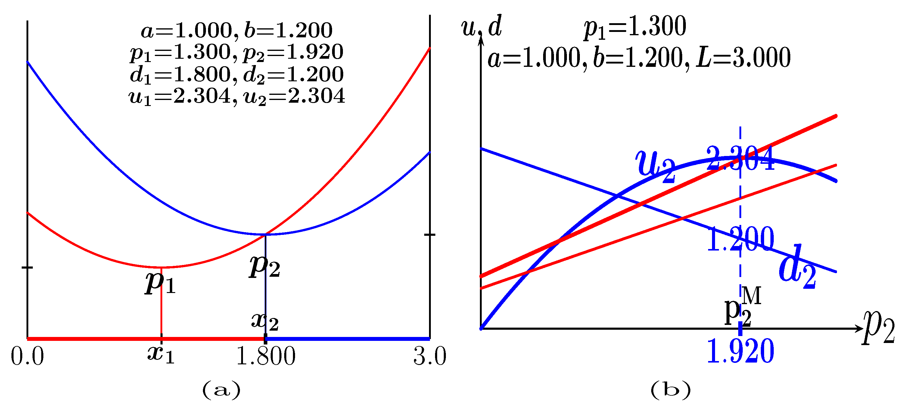
Figure 19 deals with the SHOT2-a game at a = 1.00 , L = 3.0 . Figure 19a shows that, much as in Figure 14a, it is d 2 = b , although expenses do not equalize in the ( x 2 , L ] market interval (which is not feasible with quadratic transportation cost). In Figure 19b it is p 2 M ( p 1 ) = 1 2 ( p 1 + ( L k ) d x ) = 1 2 ( 1.3 + ( 3.0 1.0 + 1.2 ) 0.8 ) = 1.920 . Note that in the game of Figure 19 it is u 1 = u 2 = 2.304 .
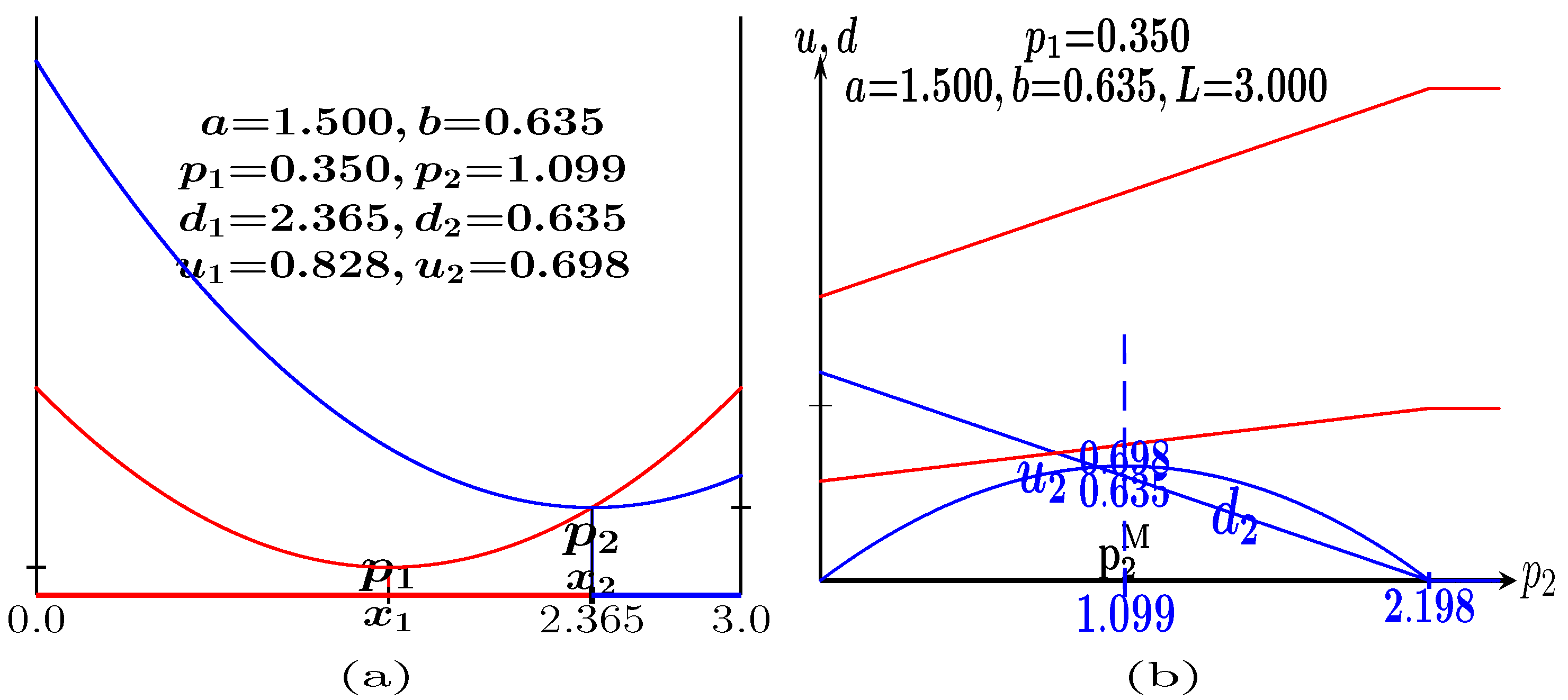
At a = 1.500 in Figure 18b it is p 1 = 0.350 , d 1 = 2.365 , b = d 2 = 0.635 , p 2 = 1.099 , u 1 = 0.828 , u 2 = 0.698 as shown in Figure 20. In Figure 20b u 2 becomes zero after the maximum when p 2 = p 1 + ( L + b a ) ( L b a ) = p 1 + ( L / 2 + b ) ( L / 2 b ) = 0.350 + ( 1.500 + 0.635 ) ( 1.500 0.635 ) = 2.198 = 2 p 2 M .
In the SHOT2-a game with a ( a 0 , L / 2 ] it is p 2 M ( p 1 ) p 2 = p 1 + ( L b a ) 2 . As a result, p 1 = ( a + 3 b L ) ( L b a ) , b = d 2 = 1 3 2 ( L a ) ( L a ) 2 3 p 1 19. Therefore, in the game of Figure 20, where a = L / 2 , it is p 2 = p 1 + ( L 2 b ) 2 = 0.350 + ( 1.500 0.635 ) 2 = 1.099 , and p 1 = ( 3 b L 2 ) ( L 2 b ) = ( 1.905 1.500 ) ( 1.500 0.635 ) = 0.350 , b = d 2 = 1 3 L ( L 2 / 4 3 p 1 13 3.000 ( 9 / 4 3 · 0.350 = 0.635 .

6. Conclusions

Numerical simulation is a powerful tool for studying the sequential Hotelling game (SHOT) where the location of the leader (SHOT-a) or that of the follower (SHOT-b) is exogenously fixed. The main findings of this article are summarized in what follows.
  • The subgame perfect equilibrium (SPE) solution exists in both scenarios regardless of the proximity of players in a finite market of length L .
  • The follower overrates the leader as a general rule. The only exception applies to the SHOT-b game with very low b , that is, in which case the leader overrates the follower to a low extent.
  • In the SHOT-b game, the advantage of the follower increases with b in a linear-like way, reaching its maximum when the follower is located in the market center.
  • In the SHOT-a game, the effect of the variation in a is quite sophisticated, so the maximum payoff of the leader is reached at a = 0.106 L , which defines the SPE solution in the location–price SHOT game.
  • In the SHOT game with quadratic transportation cost, the follower advantage notably increases compared to that found with linear transportation cost, and in the SPE solution in the location–price SHOT game, the leader shifts to his market end.
The study of the SHOT game with reservation cost [15,16] and of the SHOT game with elastic demand [14,15,17] is planned for a later study. The study of these sophisticated variants of the SHOT game will be addressed by implementing unsupervised or brute force simulation mechanisms which have already been tested in this work when dealing with the model with quadratic transportation cost.

Author Contributions

Conceptualization, L.G.-P., J.G.-C. and R.A.-S.; Validation, L.G.-P., J.G.-C. and J.C.L.; Investigation, R.A.-S.; Resources, J.C.L.; Data curation, L.G.-P.; Writing—original draft, J.G.-C. and J.C.L.; Writing—review & editing, R.A.-S. All authors have read and agreed to the published version of the manuscript.

Funding

This work has been funded by the Spanish Grant PID2021-122711NB-C21. The computations of this work were performed in FISWULF, an HPC machine of the Campus of Excellence of Moncloa.

Data Availability Statement

Data are contained within the article.

Conflicts of Interest

The authors declare no conflicts of interest.

Appendix A

Appendix A.1. Initial Simulation Iteration

Figure A1 shows the quantities involved in the initial iteration in a 5 × 5 lattice subset in the simulation of Figure 4b, that is, with x 2 = 2.25 . The snapshot under ( p 1 0 , x 1 0 )   ( p 2 0 , x 2 ) shows the initial prices of both players and of the leader locations. In the snapshot under ( p 1 1 , x 1 1 )   ( p 2 0 , x 2 ) the leader locations and prices have been updated. Thus, for example, in the box-framed central cell, the leader has changed from (9.90,0.73) into (1.24,0.93).
Figure A1. Initial iteration in a 5 × 5 lattice subset in the simulation of Figure 4. Red-marked cells are leader players and blue marked cells are follower players.
Appliedmath 05 00069 g0a1
In the snapshot under ( p 1 1 , x 1 1 )   ( p 2 0 , x 2 ) the follower prices have been updated. Thus, for example, in the box-framed cell, the follower price has changed from 9.67 into 2.16. The snapshot under ( u 1 1 , u 2 1 ) shows the payoffs in the Hotelling game after the first update. Thus, for example, the central leader player obtains the payoff:
u 1 = 3.122 = ( u 1 [ ( 1.24 , 0.93 ) , ( 2.16 , 2.25 ) ] ] u 1 [ ( 1.24 , 0.93 ) , ( 2.16 , 2.25 ) ] + u 1 [ ( 1.24 , 0.93 ) , ( 5.08 , 2.25 ) ] + u 1 [ ( 1.24 , 0.93 ) , ( 5.08 , 2.25 ) ] ) / 4 = ( 2.536 + 3.707 + 2.536 + 3.707 ) / 4 .

Appendix A.2. Patterns

Figure A2 shows the patterns of p , ( a , b ) , and u in the simulation of Figure 4b at T = 20 , where it is as follows: p ¯ 1 = 3.889 , x ¯ 1 = 0.471 , u ¯ 1 = 6.889 p ¯ 2 = 3.584 , u ¯ 2 = 6.427 . The patterns show a kind of patchwork, despite that the standard deviations of the magnitudes are quite small: σ p 1 = 0.184 , σ x 1 = 0.048 , σ u 1 = 0.079 σ p 2 = 0.110 , σ u 2 = 0.039 .
Figure A2. Patterns in the simulation of Figure 4b at T = 20 . Increasing gray levels indicate increasing values. p m i n = 3.103 , p m a x = 4.575 ; x 1 m i n = 0.284 , x 1 m a x = 0.687 ; u m i n = 3.897 , u m a x = 7.951 .
Appliedmath 05 00069 g0a2

Appendix A.3. Fortran Codes

Table A1. Code for the update of leader in the (i,j) cell in the SHOT-a game.
 SUBROUTINE SHOTALEAD(BC,WPP,p1p,i,j,n)
   double precision WPP(n,n);integer BC(0:n+1)
   COMMON /HOT/ rL,rL2,r2L,xx1
   ux=0.d0;p1p=WPP(i,j);fx2=rL2/1000.d0
   DO jj=j-1,j+1;DO ii=i-1,i+1;ik=BC(ii);jh=BC(jj)
      if(mod(ik+jh,2)==1)cycle;pp1=WPP(ik,jh)
      p2x=0.d0;x2x=0.d0;u2x=0.d0
      DO ix2=1,1001
         x2=rL2+(ix2-1)*fx2;diffx=x2-xx1;sumx=x2+xx1
         p2=pp1-diffx-0.001d0;if(p2x<0.d0) goto 1      !U
            u2=p2*rL
            if(u2>u2x)then;p2x=p2;x2x=x2;u2x=u2;endif
1       p2=(pp1+r2L-sumx)/2.d0                   !M
            call HOT(rL,pp1,p2,xx1,x2,u1,u2)
            if(u2>u2x)then;p2x=p2;x2x=x2;u2x=u2;endif
         p2=pp1+diffx-0.001d0                  !N
            call HOT(rL,pp1,p2,xx1,x2,u1,u2)
            if(u2>u2x)then;p2x=p2;x2x=x2;u2x=u2;endif
         ENDDO
         call HOT(rL,pp1,p2x,xx1,x2x,u1,u2)
         if(u1>ux)then;ux=u1;p1p=pp1;endif
      ENDDO;ENDDO
   END
Table A2. Follower update in the (i,j) cell in the SHOT-a game.
SUBROUTINE SHOTAFOLLOW(BC,WPP,WXX,p2p,x2x,i,j,n)
double precision WPP(n,n),WXX(n,n)
integer BC(0:n+1);COMMON /HOT/ rll,xx1
ux=0.d0;p2p=0.d0;x2x=0.d0
DO jj=j-1,j+1;DO ii=i-1,i+1;ik=BC(ii);jh=BC(jj)
   if(mod(ik+jh,2)==0)cycle
   p2=WPP(ik,jh);x2=WXX(ik,jh);uux=0.d0
   DO jjj=j-1,j+1;DO iii=i-1,i+1;ik=BC(iii);jh=BC(jjj)
      if(mod(ik+jh,2)==1)cycle
      p1p=WPP(ik,jh)
      call HOT(rll,p1p,p2,xx1,x2,u1,u2)
      uux=uux+u2
   ENDDO;ENDO
   if(uux>ux)then;ux=uux;p2p=p2;x2x=x2;endif
ENDDO;ENDDO
END
Table A3. Direct simulation of the SHOT-a game.
     SUBROUTINE SHOTA-SCRATCH
     integer, parameter::nsx=1000; double precision SHOTA(nsx+1,8)
     commom/HOT/ rL,rL2; rix=rL2/nsx
     plim=2.d0;if(rL==3.d0)plim=10.d0;pip=plim/nsx
     DO ia=1,nsx+1;xa=(ia-1)*rix
        uli=0.d0;pa=0.d0;xb=0.d0;pb=0.d0
        DO ipi=1,nsx+1;plix=(ipi-1)*pip
        xbx=0.d0;fop=0.d0;pli=0.d0;ufo=0.d0
           DO ixb=1,nsx+1;bx=(ixb-1)*rix
              x2=rll-bx;diffx=x2-xa
              fopx=plix-diffx-0.001d0 !————-U—————
              if(fopx<0.d0)goto 1
              u2=fopx*rll
              if(u2>ufo)then; xbx=bx;fop=fopx;pli=plix;ufo=u2; endif
1              fopx=(plix+rll-xa+bx)/2.d0 !——–M—————-
              call XHOT(rll,plix,fopx,xa,x2,u1,u2)
              if(u2>ufo)then; xbx=bx;fop=fopx;pli=plix;ufo=u2; endif
              fopx=plix+diffx-0.001d0 !————-N—————-
              call XHOT(rll,plix,fopx,xa,x2,u1,u2)
              if(u2>ufo)then; xbx=bx;fop=fopx;pli=plix;ufo=u2; endif
           ENDDO
        call HOT(rL,pli,fop,xa,rL-xbx,u1,u2)
        if(u1>uli)then; uli=u1;pa=pli;xb=xbx;pb=fop; endif
        ENDDO
        SHOTA(ia,1)=xa;SHOTA(ia,2)=pa;SHOTA(ia,3)=xb;SHOTA(ia,4)=pb
     ENDDO
     DO ia=1,nsx+1
        xa=SHOTA(ia,1);pa=SHOTA(ia,2);xb=SHOTA(ia,3);pb=SHOTA(ia,4)
        call XHOT(rL,pa,pb,xa,rL-xb,d1,d2,u1,u2)
        SHOTA(ia,5)=d1;SHOTA(ia,6)=d2;SHOTA(ia,7)=u1;SHOTA(ia,8)=u2
     ENDDO
c————– print SHOTA————
     END
Table A4. Unsupervised updating of the leader in the (i,j) cell in the SHOT-b game with quadratic transportation cost.
subroutine RAWBLEAD(bc,WPP,WXX,p1p,x1x,i,j,n)
   double precision WPP(n,n),WXX(n,n)
   integer bc(0:n+1);common/hot/rll,xx2
   ux=0.d0;p1p=WPP(i,j)
   DO jj=j-1,j+1;DO ii=i-1,i+1;ik=bc(ii);jh=bc(jj)
      if(mod(ik+jh,2)==1)cycle;pp1=WPP(ik,jh);xx1=WXX(ik,jh)
      diffx=xx2-xx1
      p2x=0.d0;u2x=0.d0;fp2=(pp1+diffx)/1000.d0
      DO ipo=1,1001
         p2=(ipo-1)*fp2
         call HOT2(rll,pp1,p2,xx1,xx2,u1,u2)
         if(u2>u2x)then;u2x=u2;p2x=p2;endif
      ENDDO
      call HOT2(rll,pp1,p2x,xx1,xx2,u1,u2)
      if(u1>ux)then;ux=u1;p1p=pp1;x1x=xx1;endif
   ENDDO;ENDDO
end

References

  1. Hotelling, H. Stability in competition. Econ. J. 1929, 39, 41–57. [Google Scholar] [CrossRef]
  2. Hinloopen, J.; Martin, S. The Hotelling Line at 95: Introduction to the Special Issue. Rev. Ind. Organ. 2024, 65, 627–648. [Google Scholar] [CrossRef]
  3. d’Aspremont, C.; Gabszewicz, J.J.; Thisse, J.F. On Hotelling’s “Stability in competition”. Econometrica 1979, 47, 1145–1150. [Google Scholar] [CrossRef]
  4. Puu, T. Hotelling’s “Ice cream dealers” with elastic demand. Ann. Reg. Sci. 2002, 36, 1–17. [Google Scholar] [CrossRef]
  5. Graitson, D. On Hotelling’s ’stability in competition’ again. Econ. Lett. 1980, 6, 1–6. [Google Scholar] [CrossRef]
  6. Iskakov, M.; Iskakov, A. Solution of the Hotelling’s game in secure strategies. Econ. Lett. 2012, 117, 115–118. [Google Scholar] [CrossRef]
  7. Shy, O. Hotelling’s Model with Firms Located Close to Each Other. Rev. Ind. Organ. 2024, 65, 649–668. [Google Scholar] [CrossRef]
  8. Puu, T.; Sushko, I. Oligopoly Dynamics: Models and Tools; Springer: Berlin/Heidelberg, Germany, 2002. [Google Scholar]
  9. Gabszewicz, J.J.; Schweizer, U.; Thisse, J.F.; Fujita, M. Location Theory; Routledge: London, UK, 2001. [Google Scholar]
  10. Anderson, S. Spatial competition and price leadership. Int. J. Ind. Organ. 1987, 5, 69–398. [Google Scholar] [CrossRef]
  11. Neven, D. Two stage (perfect) equilibrium in Hotelling’s game. J. Ind. Econ. 1985, 23, 317–325. [Google Scholar] [CrossRef]
  12. Garcia-Perez, L.; Grau-Climent, J.; Losada, J.C.; Alonso-Sanz, R. Simulation of the Stackelberg-Hotelling game. Games 2024, 15, 34. [Google Scholar] [CrossRef]
  13. Wolfram, S. A New Kind of Science; Wolfram Media: Champaign, IL, USA, 2002. [Google Scholar]
  14. Fleckinger, P.; Lafay, T. Product flexibility and price competition in Hotelling’s duopoly. Math. Soc. Sci. 2010, 60, 61–68. [Google Scholar] [CrossRef]
  15. Grau-Climent, J.; Garcia-Perez, L.; Losada, J.C.; Alonso-Sanz, R. Simulation of the Hotelling-Smithies game: Hotelling was not so wrong. Commun. Nonlinear Sci. Numer. Simul. 2022, 110, 106513. [Google Scholar] [CrossRef]
  16. Lerner, A.P.; Singer, H.W. Some notes on duopoly and spatial competition. J. Political Econ. 1937, 45, 145–186. [Google Scholar] [CrossRef]
  17. Smithies, A. Optimum location in spatial competition. J. Political Econ. 1941, 49, 423–439. [Google Scholar] [CrossRef]
1
The NE obtained in [1] is achieved at the intersection of the optimized reaction functions of the two players obtained via
derivatives. Namely, at the intersection of ( i ) u 1 p 1 = 0 p 1 = 1 2 ( p 2 + t s x ) , i.e., p 1 M ( p 2 ) = 1 2 ( p 2 + t ( L + a b ) ) , and
( i i )   u 2 p 2 = 0 p 2 = 1 2 ( p 1 + t ( 2 L s x ) ) , i.e., p 2 M ( p 1 ) = 1 2 ( p 1 + t ( L a + b ) ) .
2
u 1 U ( p 2 ) = p 2 ( L b a ) t L ; u 1 M ( p 2 ) = 1 2 ( p 2 + ( L + a b ) t ) 1 2 L b + a + p 2 1 2 ( p 2 + ( L + a b ) t ) t =
1 4 ( p 2 + ( L + a b ) t ) 1 2 L b + a + p 2 t = 1 8 p 2 ( L b + a ) + p 2 2 t + ( L + a b ) 2 t + ( L + a b ) p 2 =
1 8 1 t 2 p 2 ( L b + a ) t + p 2 2 + ( L + a b ) 2 t 2 ; u 1 U ( p 2 ) = u 1 M ( p 2 ) p 2 ( L b a ) t L 8 t = 2 p 2 ( L b + a ) t +
p 2 2 + ( L + a b ) 2 t 2 p 2 2 + 2 ( 3 L b + a ) p 2 t + ( L + a b ) 2 + 8 ( L b a ) L t 2 . Δ = ( 4 ( 3 L b + a ) 2
4 ( L + a b ) 2 + 8 ( L b a ) L ) t 2 =   4 ( 9 L 2 + b 2 + a 2 + 6 L b 6 L a 2 a b L 2 a 2 b 2 2 L a + 2 L b +
2 a b 8 L 2 + 8 b L + 8 a L ) ) t 2 = 4 · 16 L b t 2   p 2 = 1 2 2 ( 3 L + b a ) 8 L b t p ^ 2 = ( 3 L + b a 4 L b ) t .
In the location-symmetric game it is p ^ 1 = ( 3 L 4 L a ) t , in which case a 9 L / 16 supports p ^ 1 0 .
3
p 1 N < p 1 M p 2 + L b a < ( p 2 + L + a b ) / 2 p 2 < 3 a + b L > 0 , and p 2 N < p 2 M p 1 + L b a <
( p 2 + L a + b ) / 2 p 1 < 3 b + a L > 0 . Both constraints reduce in the location-symmetric game to a = b > L / 4 .
4
d 1 ( a ) = 1 2 L b + a + p 2 p 1 t u 1 ( a ) = d a p 1 .   Thus, in Figure 8a, d 1 ( a ) = 1 2 ( 3.0 0.0 + a + 3.309 4.208 ) =
1 2 ( 2.101 + a ) u 1 ( a ) = 4.208 1 2 ( 2.101 + a ) , so that u 1 ( a = 0.0 ) = 4.422 , u 1 ( a = 1.5 ) = 4.579 .In Figure 8b,
d 1 ( a ) = 1 2 ( 3.0 0.750 + a + 3.584 3.889 ) = 1 2 ( 2.555 + a ) u 1 ( a ) = 3.889 1 2 ( 2.555 + a ) , so that
u 1 ( a = 0 ) = 3.783 , u 1 ( a = 1.5 ) = 6.701 . In Figure 8c, d 1 ( a ) = 1 2 ( 3.0 1.500 + a + 3.839 3.547 ) =
1 2 ( 1.792 + a ) u 1 ( a ) = 3.547 1 2 ( 1.792 + a ) , so that u 1 ( a = 0.0 ) = 3.180 . In Figure 8c, x 2 x 1 = p 2 p 1 becomes
3.0 1.5 a = 3.839 3.47 = 0.279 a = 1.208 , so that with a > 1.208 it is d 1 = 3.0 u 1 = 3.0 · 3.547 = 10.641 .
5
From Equations (5b) and (5c), 1 t p 2 p 2 = 1 2 ( p 1 + ( L a + b ) ) = 1 2 ( 3 L a + b + 4 L a + L a + b ) =
L + b a + 2 L a ) d 1 = 1 2 L b + a L + b a + 2 L a = L a .
6
From a generic a , it is u 1 = L a 3 L + a b 4 L a t . Thus, u 1 a = t L 3 L + 3 a b 8 L a   u 1 a = 0
3 a 8 L a + 3 L b = 0   a = 4 L 7 L + 3 b 3 a = 23 L + 3 b 8 7 L + 3 b 9 .
7
1 t ( p 2 # p 1 # ) = 1 2 1 t p 1 # + ( 3 L 2 a # ) = 1 2 5 L 2 a # + 4 L a # + 3 L 2 a # = L 2 a # + 2 L a # d 1 =
1 2 L 2 + a # L 2 a # + 2 L a # = L 0.1307 L = 0.3615 L .
8
This value arises from 3 L + a b = 8 L a with b = L / 2 , that is, from 5 2 L + a 2 = 64 L a .
9
Note that there is no value discontinuity in the prices at a = a 0 . Thus, for example, in the case of L = 3 at a 0 = 0.318 it
is as follows: p 1 = 1 2 5 2 3 + 0.318 = 5 2 3 + 0.318 4 3 · 0.318 = 3.909 and p 2 = 1 4 11 2 3 0.318 =
2 3 4 3 · 0.318 = 4.046
10
This may be proven by maximizing the u 1 given in Equation (10b) or just referring to footnote 7 in the particular case of
b = L / 2
11
u 2 ( p 1 , p 2 N ( p 1 ) ) = ( p 1 + ( L b a ) ) L 1 2 s x + ( L b a ) = p 2 L 1 2 L b + a + L b a = p 1 +
( L b a ) b .       u 2 b = ( p 1 + L b a ) b u 2 b = 0   b = 1 2 ( p 1 + L a ) = p 2 = p 1 + L 1 2 ( p 1 + L a ) a
12
d 1 ( p 1 , p 2 ( p 1 ) = b ( p 1 ) ) = 1 2 L p 2 + a + ( p 2 p 1 ) = 1 2 ( L + a p 1 ) d 2 = 1 2 ( p 1 + L a ) . It is p + L b a =
p 2 = b p 1 = 2 b + a L
13
p 1 + ( L L 2 a ) L = p 1 + ( L 1 2 ( p 1 + L a ) a ) 1 2 ( p 1 + L a ) p 1 = L + a 2 L ( 4 a L ) ̲ . Note that at
a = 3 8 L it is, b = p 2 = d 2 = L 1 2 2 L ( 4 3 8 L L ) = L 1 2 L = 1 2 L , and p 1 = L + 3 8 L 2 L ( 4 3 8 L L ) = 11 8 L
1 2 L = 3 8 L . Therefore, there is no discontinuity in the values of the variables at a = 3 8 L . Moreover, if a < 3 8 L it is
b > 1 2 L according to Equation (12a). That is why it is b = 1 2 L when a < 3 L / 8 .
14
In Figure 13 at a = L / 2 , with L = 1 it is p 1 = 0.088 , d 1 = 0.706 , p 2 = d 2 = b = 0.293 , u 1 = 0.062 < u 2 = 0.086 , and
with L = 3 it is p 1 = 0.280 , d 1 = 2.100 , p 2 = 0.880 d 2 = b = 0.900 , u 1 = 0.588 < u 2 = 0.792 .
15
s ¯ = 0 = s x + p 2 p 1 t d x p 2 = p 1 s x d x t ;     s ¯ = L = s x + p 2 p 1 t d x p 1 = p 2 ( L s x ) d x t .
16
  u 1 = u 2 1 16 ( 3 L + k ) 2 = 1 32 ( 5 L k ) 2 2 ( 3 L + k ) = 5 L k k = 5 3 2 1 + 2 L = 0.314 L .
17
p 2 U = p 1 s x d x t = 9.232 2.276 · 2.224 = 4.170 . It is s ¯ = L 2 L = s x + p 2 p 1 t d x p 2 = p 1 + ( 2 L s x ) d x t ; therefore, p 1 = 9.232 undercuts player 2 when p 2 > 9.2232 + ( 6.000 2.276 ) 2.224 = 17.514 in Figure 16c, far beyond
the scope of p 2 in this figure.
18
With L = 1.0 it is p 1 = 0.024 , b = 0.194 , p 2 = 0.118 , u 1 = 0.024 · 0.807 = 0.019 < 0.118 · 0.193 = 0.023 = u 2 ; and
with L = 3.0 it is p 1 = 0.240 , b = 0.582 , p 2 = 1.080 , u 1 = 0.210 · 2.422 = 0.509 < 1.060 · 0.578 = 0.613 = u 2 .
19
1 2 ( p 1 + ( L k ) d x ) = p 1 + d x 2 p 1 = ( L k ) d x 2 d x 2 = ( L a + b 2 L + 2 b + 2 a ) d x = ( a + 3 b L ) ( L b a ) ̲ .
Additionally, u 2 = ( p 1 + d x 2 ) b . Therefore, u 2 b = 0 b = 1 3 2 ( L a ) ( L a ) 2 3 p 1 .
Figure 1. The HOT game.
Appliedmath 05 00069 g001
Figure 2. The backwards induction principle in price variables.
Appliedmath 05 00069 g002
Figure 3. The layout of the interactions in the numerical simulation. (a) Leader updating. (b) Follower updating. (c) Game play. Arrows indicate cell interactions.
Appliedmath 05 00069 g003
Figure 4. Dynamics in the simulation of the SHOT-b game. L = 3.0 , t = 1.0 . Five simulations. (a) b = 0.00 . (b) b = 0.75 . (c) b = 1.50 .
Appliedmath 05 00069 g004
Figure 5. The HOT game in the steady state of the simulation of Figure 4a. (a) The game at T = 20 . (b) The game with variable p 1 and p 2 = 3.309 . (c) The game with variable p 2 and p 1 = 4.208 .
Appliedmath 05 00069 g005
Figure 6. The HOT game in the steady state of the simulation of Figure 4b. (a) The game at T = 20 . (b) The game with variable p 1 and p 2 = 3.584 . (c) The game with variable p 2 and p 1 = 3.889 .
Appliedmath 05 00069 g006
Figure 7. The HOT game in the steady state of the simulation of Figure 4c. (a) The game at T = 20 . (b) The game with variable p 1 and p 2 = 3.839 . (c) The game with variable p 2 and p 1 = 3.547 .
Appliedmath 05 00069 g007
Figure 8. a -responses in the HOT game given b and prices. (a) b = 0.00 . (b) b = 0.75 . (c) b = 1.5 .
Appliedmath 05 00069 g008
Figure 9. Simulation of the SHOT-b game with parameterized b . T = 20 . Five initial configurations. (a) L = 1.0 . (b) L = 3.0 .
Appliedmath 05 00069 g009
Figure 10. Simulation of the SHOT-a game with parameterized a . T = 20 . (a) L = 1.0 . (b) L = 3.0 .
Appliedmath 05 00069 g010
Figure 11. The SHOT-a=0.0 game. L = 3.0 . (a) Dynamics in five simulations up to T = 20 . (b) The game with the average values values at T = 20 . (c) The game with variable p 2 and p 1 = 3.750 .
Appliedmath 05 00069 g011
Figure 12. The SHOT-a=0.75 game. L = 3.0 . (a) Dynamics in five simulations up to T = 20 . (b) The game with the simulation average variables at T = 20 . (c) The game with variable p 2 and p 1 = 2.250 .
Appliedmath 05 00069 g012
Figure 13. The SHOT-a game with parameterized a from direct simulation. (a) L = 1.0 . (b) L = 3.0 .
Appliedmath 05 00069 g013
Figure 14. The SHOT-a=0.85 game. L = 3.0 . (a) The game. (b) p 2 -response with p 1 = 1.960 .
Appliedmath 05 00069 g014
Figure 15. Simulation of the SHOT2-b game with parameterized b . T = 20 . (a) L = 1.0 . (b) L = 3.0 .
Appliedmath 05 00069 g015
Figure 16. The SHOT2- b = 0.75 game from Figure 15b. (a) Dynamics in the simulation. (b) The game at T = 20 . (c) The game with variable p 2 and p 1 = 9.232 .
Appliedmath 05 00069 g016
Figure 17. Simulation of the SHOT2-a game with parameterized a . T = 20 . (a) L = 1.0 . (b) L = 3.0 .
Appliedmath 05 00069 g017
Figure 18. The SHOT2-a game with parameterized a from direct simulation. (a) L = 1.0 . (b) L = 3.0 .
Appliedmath 05 00069 g018
Figure 19. The SHOT2-a = 1.0 game. L = 3.0 . (a) The SPE solution of the game. (b) p 2 -response to ( a = 1.000 , p 1 = 1.300 ) from b = 1.200 .
Appliedmath 05 00069 g019
Figure 20. The SHOT2-a = 1.5 game. L = 3.0 . (a) The SPE solution of the game. (b) p 2 -response to ( a = 1.500 , p 1 = 0.350 ) from b = 0.635 .
Appliedmath 05 00069 g020
Table 1. Leader update of the (i,j) cell in the SHOT-b game.
subroutine SHOTBLEAD(bc,WPP,WXX,p1p,x1x,i,j,n)
   double precision WPP(n,n),WXX(n,n);integer bc(0:n+1)
   common /hot/rL,r2L,xx2
   ux=0.d0;p1p=WPP(i,j);x1x=WXX(i,j)
   DO jj=j-1,j+1;DO ii=i-1,i+1;ik=bc(ii);jh=bc(jj)
      if(mod(ik+jh,2)==1)cycle
      pp1=WPP(ik,jh);xx1=WXX(ik,jh)
      p2x=0.d0;u2x=0.d0
      diffx=xx2-xx1;sumx=xx2+xx1
      p2=pp1-diffx-0.001d0;if(p2x<0.d0) goto 1       !U
            u2=p2*rL
            if(u2>u2x)then;p2x=p2;u2x=u2;endif
1   p2=(pp1+r2L-sumx)/2.d0                                  !M
            call HOT(rL,pp1,p2,xx1,xx2,u1,u2)
            if(u2>u2x)then;p2x=p2;u2x=u2;endif
      p2=pp1+diffx-0.001d0                                         !N
            call HOT(rL,pp1,p2,xx1,xx2,u1,u2)
            if(u2>u2x)then;p2x=p2;u2x=u2;endif
      call HOT(rL,pp1,p2x,xx1,xx2,u1,u2)
      if(u1>ux)then;ux=u1;p1p=pp1;x1x=xx1;endif
   ENDDO;ENDDO
end
Table 2. Update of the follower in the (i,j) cell in the SHOT-b game.
suboutine SHOTBFOLLOW(BC,WPP,WXX,p2p,i,j,n)
      double precision WPP(n,n),WXX(n,n)
      integer BC(0:n+1); common/hot/rL,xx2
      ux=0.d0;p2p=0.d0
      DO jj=j-1,j+1;DO ii=i-1,i+1;ik=BC(ii);jh=BC(jj)
            if(mod(ik+jh,2)==0)cycle
            p2=WPP(ik,jh);uux=0.d0
            DO jjj=j-1,j+1;DO iii=i-1,i+1;ik=BC(iii);jh=BC(jjj)
                  if(mod(ik+jh,2)==1)cycle
                  p1p=WPP(ik,jh);x1x=WXX(ik,jh)
                  call HOT(rL,p1p,p2,x1x,xx2,u1,u2)
                  uux=uux+u2
            ENDDO;ENDDO
            if(uux>ux)then;ux=uux;p2p=p2;endif
      ENDDO;ENDDO
end
Disclaimer/Publisher’s Note: The statements, opinions and data contained in all publications are solely those of the individual author(s) and contributor(s) and not of MDPI and/or the editor(s). MDPI and/or the editor(s) disclaim responsibility for any injury to people or property resulting from any ideas, methods, instructions or products referred to in the content.