An Alternative Framework for Dynamic Mode Decomposition with Control

Abstract

Dynamic mode decomposition with control (DMDc) is a widely used technique for analyzing dynamic systems influenced by external control inputs. It is a recent development and an extension of dynamic mode decomposition (DMD) tailored for input–output systems. In this work, we investigate and analyze an alternative approach for computing DMDc. Compared to the traditional formulation, the proposed method restructures the computation by decoupling the influence of the state and control components, allowing for a more modular and interpretable implementation. The algorithm avoids compound operator approximations typical of standard approaches, which makes it potentially more efficient in real-time applications or systems with streaming data. The new scheme aims to improve computational efficiency while maintaining the reliability and accuracy of the decomposition. We provide a theoretical proof that the dynamic modes produced by the proposed method are exact eigenvectors of the corresponding Koopman operator. Compared to the standard DMDc approach, the new algorithm is shown to be more efficient, requiring fewer calculations and less memory. Numerical examples are presented to demonstrate the theoretical results and illustrate potential applications of the modified approach. The results highlight the promise of this alternative formulation for advancing data-driven modeling and control in various engineering and scientific domains.

1. Introduction

With advancements in technology, capabilities in data storage, transfer rates, and computational power are rapidly increasing, leading to the generation of massive datasets. This creates a growing need for new techniques for the real-time control of complex systems. The modeling and control of such systems are central to various applications in physical, biological, and engineering domains. These include epidemic control, internet traffic regulation, energy infrastructure optimization, and more.

The analysis and control of complex systems require the development of innovative quantitative methods and data-driven techniques. One such approach is dynamic mode decomposition (DMD) [1], which has become a prominent tool for identifying spatiotemporal coherent structures from high-dimensional data. DMD provides a numerical approximation to Koopman spectral analysis and can therefore be applied to nonlinear dynamical systems [2,3]. Over the past decade, the DMD method has gained popularity across a wide range of applications, including video processing [4], epidemiology [5], neuroscience [6], financial trading [7,8,9], robotics [10], cavity flows [11,12], and various jet flows [2,13]. For an overview of the DMD literature, we refer the reader to [14,15,16,17].

In recent years, a variety of advanced control strategies and mathematical models have been proposed to address complex systems in different fields. For instance, Liang et al. [18] explored decentralized control for networked systems under asymmetric information conditions, while Fahim et al. [19] developed a mathematical framework for liquidity risk contagion in banking systems using optimal control approaches. Shahgholian and Fathollahi [20] focused on improving load frequency control in multi-resource energy systems, particularly through superconducting magnetic energy storage, and Ndeke et al. [21] provided a detailed methodology for modeling voltage source converters in electrical circuits.

In practical settings, the modeling of high-dimensional, complex dynamical systems often requires accounting for external inputs or control actions. The standard DMD framework does not include control effects and may therefore fail to accurately predict system behavior under actuation. To address this, a modification known as dynamic mode decomposition with control (DMDc) was proposed in [22]. DMDc incorporates both state measurements and external inputs to capture the underlying system dynamics. In this work, we present an alternative formulation for implementing the DMDc method. Before introducing the new approach, we will briefly review the standard DMD and DMDc methodologies.

1.1. Dynamic Mode Decomposition (DMD Method)

For completeness, we begin with a brief overview of the standard DMD framework, following the formulation in [14]. Let us consider a sequential set of snapshot vectors:

$$D=\{{\mathbf{x}}_0,\dots ,{\mathbf{x}}_m\},$$

(1)

where each snapshot ${\mathbf{x}}_k\in {\mathbb{R}}^n$. These data vectors may originate from simulations, experiments, or real-world measurements collected at discrete times $t_k$, assumed to be uniformly spaced by a time interval $\Delta t$, over the interval $[t_0,t_m]$.

The DMD method begins by arranging the data into two large matrices:

$$X=[{\mathbf{x}}_0,\dots ,{\mathbf{x}}_{m-1}],Y=[{\mathbf{x}}_1,\dots ,{\mathbf{x}}_m].$$

(2)

The central assumption of the method is that a linear operator A exists such that we have the following:

$${\mathbf{x}}_{k+1}=A{\mathbf{x}}_k,$$

(3)

which, in matrix form, leads to:

$$Y=AX.$$

(4)

Performing spectral decomposition of A yields the so-called dynamic mode decomposition of the dataset be italic D. The eigenvectors and eigenvalues of A are approximated and referred to as the DMD modes and DMD eigenvalues, respectively.

To compute the best-fit approximation of A, we apply the Moore–Penrose pseudoinverse $X^{†}$ to both sides of Equation (4):

$$A\approx Y{X}^{†}.$$

(5)

A practical approach for computing this approximation uses the singular value decomposition (SVD) of $X=U_X{\Sigma }_X{V}_X^{\ast }$:

$$A\approx Y{V}_X{\Sigma }_X^{-1}{U}_X^{\ast },$$

(6)

where $U_X\in {\mathbb{R}}^{n\times n}$ and $V_X\in {\mathbb{R}}^{m\times m}$ are unitary matrices, and ${\Sigma }_X\in {\mathbb{R}}^{n\times m}$ is a diagonal matrix of singular values. The symbol * denotes complex conjugate transpose.

In high-dimensional settings where $n\gg m$, direct analysis of A becomes computationally expensive. DMD addresses this by projecting A onto a lower-dimensional subspace using a reduced SVD. This is motivated by the often low-dimensional nature of the essential system dynamics.

Let the reduced (or truncated) SVD of X be as follows:

$$X\approx U_r{\Sigma }_r{V}_r^{\ast },$$

(7)

where r is the truncation rank, $U_r\in {\mathbb{R}}^{n\times r}$, ${\Sigma }_r\in {\mathbb{R}}^{r\times r}$, and $V_r\in {\mathbb{R}}^{m\times r}$. Substituting into Equation (5), we obtain a reduced-order representation of A. By taking the basis transformation $U_r^{\ast }X=\tilde{X}$, the reduced-order model can be derived:

$$U_r^{\ast }Y=U_r^{\ast }AX=U_r^{\ast }Y{V}_r{\Sigma }_r^{-1}{U}_r^{\ast }X=\tilde{A}\tilde{X},$$

which yields the following:

$$\tilde{Y}=\tilde{A}\tilde{X},$$

(8)

where $\tilde{A}=U_r^{\ast }Y{V}_r{\Sigma }_r^{-1}$ and $\tilde{X}=U_r^{\ast }X$ are the reduced operator and reduced snapshot matrix, respectively.

By performing eigendecomposition on $\tilde{A}$:

$$\tilde{A}W=W\mathrm{\Lambda },$$

(9)

we obtain the eigenvalues $\mathrm{\Lambda }$ and eigenvectors W of the reduced system. Notably, the eigenvalues of $\tilde{A}$ are also eigenvalues of the original matrix A.

To compute the DMD modes of the full system, we lift the reduced eigenvectors back into the original space. Two formulations are commonly used:

• The exact DMD modes, introduced by Tu et al. [14]:

  $$\mathrm{\Phi }=Y{V}_r{\Sigma }_r^{-1}W,$$

  (10)
• The projected DMD modes, as originally proposed in [1]:

  $$\mathrm{\Phi }=U_{r}W.$$

  (11)

The modes from Equation (10) are exact eigenvectors of A, while those from Equation (11) represent their projection onto the POD subspace.

1.2. Dynamic Mode Decomposition with Control (DMDc)

Dynamic mode decomposition with control (DMDc) is an extension of the classical DMD method, developed to analyze multidimensional systems that are influenced by external inputs or disturbances [22]. Unlike standard DMD, which considers only the autonomous system dynamics, DMDc incorporates time-dependent control inputs, enabling it to distinguish between internal system behavior and input-driven effects.

To account for the control influence, a new data matrix—analogous to the snapshot matrices X and Y from (2)—is introduced:

$$\Gamma =[{\mathbf{u}}_0,\dots ,{\mathbf{u}}_{m-1}],$$

(12)

where each ${\mathbf{u}}_i\in {\mathbb{R}}^q$, and q is the number of input variables.

The DMDc model assumes a linear relationship between consecutive system states and the inputs:

$${\mathbf{x}}_{k+1}=A{\mathbf{x}}_k+B{\mathbf{u}}_k,$$

(13)

where $A\in {\mathbb{R}}^{n\times n}$ is the system (DMD) operator, and $B\in {\mathbb{R}}^{n\times q}$ is the input matrix. Using snapshot matrices, this model can be written as follows:

$$Y=AX+B\Gamma .$$

(14)

Assuming A and B are unknown, we rewrite Equation (14) in block matrix form:

$$Y=\left[\begin{array}{cc}A& B\end{array}\right]\left[\begin{array}{c}X\\ \Gamma \end{array}\right]=G\mathrm{\Omega },$$

(15)

where

$$G=\left[AB\right]\in {\mathbb{R}}^{n\times (n+q)},\mathrm{\Omega }=\left[\begin{array}{c}X\\ \Gamma \end{array}\right]\in {\mathbb{R}}^{(n+q)\times m}.$$

(16)

The DMDc procedure seeks the best-fit approximation of G that satisfies the relation $Y\approx G\mathrm{\Omega }$. To achieve this, we apply a truncated singular value decomposition (SVD) to the matrix $\mathrm{\Omega }$:

$$\mathrm{\Omega }\approx U_{\mathrm{\Omega }}{\Sigma }_{\mathrm{\Omega }}{V}_{\mathrm{\Omega }}^{\ast },$$

(17)

where $U_{\mathrm{\Omega }}\in {\mathbb{R}}^{(n+q)\times p}$, ${\Sigma }_{\mathrm{\Omega }}\in {\mathbb{R}}^{p\times p}$, and $V_{\mathrm{\Omega }}\in {\mathbb{R}}^{m\times p}$.

Using this decomposition, the matrix G is approximated by the following:

$$G\approx Y{V}_{\mathrm{\Omega }}{\Sigma }_{\mathrm{\Omega }}^{-1}{U}_{\mathrm{\Omega }}^{\ast }.$$

(18)

We partition $U_{\mathrm{\Omega }}$ as follows:

$$U_{\mathrm{\Omega }}=\left[\begin{array}{c}{U}_1\\ U_2\end{array}\right],$$

with $U_1\in {\mathbb{R}}^{n\times p}$ and $U_2\in {\mathbb{R}}^{q\times p}$. The matrices A and B are then approximated as follows:

$$\overline{A}\approx Y{V}_{\mathrm{\Omega }}{\Sigma }_{\mathrm{\Omega }}^{-1}{U}_1^{\ast },\overline{B}\approx Y{V}_{\mathrm{\Omega }}{\Sigma }_{\mathrm{\Omega }}^{-1}{U}_2^{\ast }.$$

(19)

To obtain a reduced-order representation of the dynamics, we project the system onto a lower-dimensional subspace. Unlike standard DMD, where the projection is based on X, here, we use the SVD of Y to define the transformation:

$$Y\approx U_Y{\Sigma }_Y{V}_Y^{\ast },$$

(20)

where $U_Y\in {\mathbb{R}}^{n\times r}$, ${\Sigma }_Y\in {\mathbb{R}}^{r\times r}$, and $V_Y\in {\mathbb{R}}^{m\times r}$. Typically, the reduced dimension, r, is smaller than p from the decomposition of $\mathrm{\Omega }$.

Applying this projection yields reduced-order operators:

$$\begin{array}{cc}\hfill \tilde{A}& =U_Y^{\ast }\overline{A}{U}_Y=U_Y^{\ast }Y{V}_{\mathrm{\Omega }}{\Sigma }_{\mathrm{\Omega }}^{-1}{U}_1^{\ast }{U}_Y,\hfill \\ \hfill \tilde{B}& =U_Y^{\ast }\overline{B}=U_Y^{\ast }Y{V}_Y{\Sigma }_Y^{-1}{U}_2^{\ast },\hfill \end{array}$$

(21)

with $\tilde{A}\in {\mathbb{R}}^{r\times r}$ and $\tilde{B}\in {\mathbb{R}}^{r\times q}$. Alternatively, one may choose to project using the SVD of X, but this leads to a different reduced basis.

The DMD modes are derived from the eigendecomposition of $\tilde{A}$:

$$\tilde{A}W=W\mathrm{\Lambda },$$

(22)

where the eigenvalues $\mathrm{\Lambda }$ describe the system’s temporal behavior, and the DMDc modes are obtained via the following:

$$\mathrm{\Phi }=Y{V}_Y{\Sigma }_Y^{-1}{U}_1^{\ast }{U}_{\mathrm{\Omega }}W.$$

(23)

The following algorithm (Algorithm 1) summarizes the steps of implementing the DMDc scheme:

Algorithm 1 Standard DMDc procedure

Collect data and construct the matrices X, Y, and $\Gamma$ as in (2) and (12). Define the combined matrix $\mathrm{\Omega }$ as in (16). Perform reduced SVD of $\mathrm{\Omega }$: $$\mathrm{\Omega }\approx U_{\mathrm{\Omega }}{\Sigma }_{\mathrm{\Omega }}{V}_{\mathrm{\Omega }}^{\ast },$$ truncated to rank p. Perform reduced SVD of Y: $$Y\approx U_Y{\Sigma }_Y{V}_Y^{\ast },$$ truncated to rank r. Compute the reduced-order operators: $$\begin{array}{cc}\hfill \tilde{A}& =U_Y^{\ast }Y{V}_{\mathrm{\Omega }}{\Sigma }_{\mathrm{\Omega }}^{-1}{U}_1^{\ast }{U}_Y,\hfill \\ \hfill \tilde{B}& =U_Y^{\ast }Y{V}_Y{\Sigma }_Y^{-1}{U}_2^{\ast }.\hfill \end{array}$$ Compute the spectral decomposition of $\tilde{A}$: $$\tilde{A}W=W\mathrm{\Lambda }.$$ Calculate the DMDc modes: $$\mathrm{\Phi }=Y{V}_Y{\Sigma }_Y^{-1}{U}_1^{\ast }{U}_{\mathrm{\Omega }}W.$$

2. Alternative DMDc Algorithm

To obtain a low-rank approximation of the operator A from Equation (13), the standard DMDc algorithm exploits the low-dimensional structure of the data. In this section, we propose an alternative formulation of the DMDc method, as also presented in [23].

Let the data matrices X, Y, and $\Gamma$ be defined as in Equations (2) and (12). Define the block matrix $\mathrm{\Omega }$ as in (16). We aim to compute the best-fit linear operator G from Equation (16) using the Moore–Penrose pseudoinverse:

$$G=Y{\mathrm{\Omega }}^{†},$$

(24)

where ${\mathrm{\Omega }}^{†}$ denotes the pseudoinverse of $\mathrm{\Omega }$. If the rows of $\mathrm{\Omega }$ are linearly independent, ${\mathrm{\Omega }}^{†}$ can be computed via SVD or as ${\mathrm{\Omega }}^{\ast }{\left(\mathrm{\Omega }{\mathrm{\Omega }}^{\ast }\right)}^{-1}$.

We now express ${\mathrm{\Omega }}^{†}$ in block form to separate the contributions of the state and control inputs:

$${\mathrm{\Omega }}^{†}=\left[\begin{array}{cc}{\mathrm{\Omega }}_1& {\mathrm{\Omega }}_2\end{array}\right],$$

(25)

where ${\mathrm{\Omega }}_1\in {\mathbb{R}}^{m\times n}$ corresponds to the state snapshot matrix X, and ${\mathrm{\Omega }}_2\in {\mathbb{R}}^{m\times q}$ corresponds to the control input matrix $\Gamma$. This decomposition allows us to isolate the influence of X and $\Gamma$ on Y.

Substituting into (24), the operators A and B are approximated as follows:

$$A\approx \widehat{A}=Y{\mathrm{\Omega }}_1,B\approx \widehat{B}=Y{\mathrm{\Omega }}_2,$$

(26)

where $\widehat{A}$ and $\widehat{B}$ are the least-squares estimates of the system and input matrices, obtained from projecting Y onto the subspaces of X and $\Gamma$.

If a reduced SVD of $\mathrm{\Omega }$ as in (17) is used, then the estimates $\widehat{A}$ and $\widehat{B}$ coincide with the matrices $\overline{A}$ and $\overline{B}$ defined in (19).

We now perform a reduced-order SVD on ${\mathrm{\Omega }}_1$ (instead of Y) to obtain a compact representation of the system dynamics:

$${\mathrm{\Omega }}_1\approx \widehat{U}\widehat{\Sigma }{\widehat{V}}^{\ast },$$

(27)

where $\widehat{U}\in {\mathbb{R}}^{m\times r}$ contains the leading left singular vectors, $\widehat{\Sigma }\in {\mathbb{R}}^{r\times r}$ is a diagonal matrix with the top r singular values, and $\widehat{V}\in {\mathbb{R}}^{n\times r}$ contains the right singular vectors. The truncation parameter r defines the rank of the reduced subspace.

Using this decomposition, we define reduced-order approximations of A and B via projection onto the subspace defined by $\widehat{V}$:

$$\begin{array}{cc}\hfill \tilde{A}& ={\widehat{V}}^{\ast }\widehat{A}\widehat{V}={\widehat{V}}^{\ast }Y\widehat{U}\widehat{\Sigma },\hfill \\ \hfill \tilde{B}& ={\widehat{V}}^{\ast }\widehat{B}={\widehat{V}}^{\ast }Y{\mathrm{\Omega }}_2,\hfill \end{array}$$

(28)

where $\tilde{A}\in {\mathbb{R}}^{r\times r}$ and $\tilde{B}\in {\mathbb{R}}^{r\times q}$ are reduced approximations of the system and input matrices. Note that this reduced-order formulation differs from the one in (21) obtained via the standard DMDc method.

We compute the eigenstructure of $\tilde{A}$:

$$\tilde{A}W=W\mathrm{\Lambda },$$

(29)

where W contains the eigenvectors of $\tilde{A}$ and $\mathrm{\Lambda }$ is a diagonal matrix of its eigenvalues.

To reconstruct the DMD modes in the full state space, we apply the following transformation:

$$\mathrm{\Phi }=Y\widehat{U}\widehat{\Sigma }W,$$

(30)

where the columns of $\mathrm{\Phi }$ are the DMD modes of the approximated operator A.

We then summarize the results in the next algorithm Algorithm 2:

Algorithm 2 Alternative DMDc Algorithm

Collect data and construct the matrices X, Y, and $\Gamma$ as in (2) and (12). Define $\mathrm{\Omega }$ as in (16). Compute the pseudoinverse ${\mathrm{\Omega }}^{†}$ and express it in block form: $${\mathrm{\Omega }}^{†}=\left[\begin{array}{cc}{\mathrm{\Omega }}_1& {\mathrm{\Omega }}_2\end{array}\right].$$ Perform a truncated SVD of ${\mathrm{\Omega }}_1$: $${\mathrm{\Omega }}_1\approx \widehat{U}\widehat{\Sigma }{\widehat{V}}^{\ast },$$ with truncation rank r. Compute the reduced-order operators: $$\begin{array}{cc}\hfill \tilde{A}& ={\widehat{V}}^{\ast }Y\widehat{U}\widehat{\Sigma },\hfill \\ \hfill \tilde{B}& ={\widehat{V}}^{\ast }Y{\mathrm{\Omega }}_2.\hfill \end{array}$$ Compute the eigendecomposition of $\tilde{A}$: $$\tilde{A}W=W\mathrm{\Lambda }.$$ Reconstruct the DMD modes: $$\mathrm{\Phi }=Y\widehat{U}\widehat{\Sigma }W.$$

In what follows, we will demonstrate that Algorithm 2 identifies all nonzero eigenvalues of the operator A. We begin by proving the following theorem.

Theorem 1.

Let the matrix $\tilde{A}$, defined in (28), have an eigenpair $(\lambda ,\mathbf{w})$, where $\lambda \ne 0$. Then the pair $(\lambda ,\varphi )$ is an eigenpair of A, where we have the following:

$$\varphi =Y\widehat{U}\widehat{\Sigma }\mathbf{w}.$$

(31)

Proof. 

We aim to show that if $\tilde{A}\mathbf{w}=\lambda \mathbf{w}$, then $\varphi$, defined via (31), satisfies $A\varphi =\lambda \varphi$, i.e., it is an eigenvector of A with eigenvalue $\lambda$.

Recall from (26) that we approximate: $A\approx \widehat{A}=Y{\mathrm{\Omega }}_1$. Also, from the reduced SVD in (27), we have: ${\mathrm{\Omega }}_1\approx \widehat{U}\widehat{\Sigma }{\widehat{V}}^{\ast }$. Combining these, we write the action of A on $\varphi$ as follows:

$$A\varphi =Y{\mathrm{\Omega }}_1\varphi =Y\widehat{U}\widehat{\Sigma }{\widehat{V}}^{\ast }\varphi .$$

Then, substituting the definition of $\varphi$ from (31):

$$A\varphi =Y\widehat{U}\widehat{\Sigma }{\widehat{V}}^{\ast }Y\widehat{U}\widehat{\Sigma }\mathbf{w}$$

We now observe that this expression is equivalent to applying the matrix $\tilde{A}={\widehat{V}}^{\ast }Y\widehat{U}\widehat{\Sigma }$, as defined in (28). Hence, we have the following:

$$A\varphi =Y\widehat{U}\widehat{\Sigma }\left(\tilde{A}\mathbf{w}\right)$$

Since $(\lambda ,\mathbf{w})$ is an eigenpair of $\tilde{A}$, we have the following:

$$A\varphi =\lambda Y\widehat{U}\widehat{\Sigma }\mathbf{w}=\lambda \varphi .$$

Thus, $\varphi$ satisfies the eigenvalue equation for A.

It remains to verify that $\varphi \ne 0$. Suppose $\varphi =0$, i.e.,

$$Y\widehat{U}\widehat{\Sigma }\mathbf{w}=0.$$

Then, multiplying both sides by ${\widehat{V}}^{\ast }$, we obtain the following:

$$\tilde{A}\mathbf{w}={\widehat{V}}^{\ast }Y\widehat{U}\widehat{\Sigma }\mathbf{w}=0,$$

which implies $\lambda =0$, contradicting the assumption $\lambda \ne 0$. Hence, $\varphi \ne 0$, and we conclude that $(\lambda ,\varphi )$ is indeed an eigenpair of A. The theorem is proved.    □

We will now show that Algorithm 2 produces all non-zero eigenvalues of A. Let us assume that $A\varphi =\lambda \varphi$, for $\lambda \ne 0$, and $\mathbf{w}={\widehat{V}}^{\ast }\varphi$. Hence

$$\tilde{A}\mathbf{w}={\widehat{V}}^{\ast }Y\widehat{U}\widehat{\Sigma }\mathbf{w}={\widehat{V}}^{\ast }Y\widehat{U}\widehat{\Sigma }{\widehat{V}}^{\ast }\varphi ={\widehat{V}}^{\ast }A\varphi =\lambda {\widehat{V}}^{\ast }\varphi =\lambda \mathbf{w}.$$

Therefore, $\mathbf{w}\ne 0$, because if ${\widehat{V}}^{\ast }\varphi =0$, then $Y\widehat{U}\widehat{\Sigma }{\widehat{V}}^{\ast }\varphi =A\varphi =0$, and $\lambda =0$. Hence, $\mathbf{w}$ is an eigenvector of $\tilde{A}$ with the corresponding eigenvalue $\lambda$, and it is discovered by Algorithm 2.

The alternative DMDc algorithm constructs a low-rank approximation of the system operator A by projecting the data onto a reduced subspace derived from the singular value decomposition (SVD) of the input data matrix. This approach yields a reduced-order operator $\tilde{A}$ that captures the dominant system dynamics. The corresponding eigenvectors are then lifted back to the original state space via the transformation $\mathrm{\Phi }=Y\widehat{U}\widehat{\Sigma }W$, recovering the DMD modes.

However, due to the nature of this projection, only the nonzero eigenvalues of A are preserved. Eigenvectors associated with zero eigenvalues are mapped to the zero vector and effectively discarded, as the transformation $\mathrm{\Phi }=Y\widehat{U}\widehat{\Sigma }W$ inherently maps any eigenvector associated with a zero eigenvalue to the zero vector. While this filtering enhances numerical robustness by eliminating uninformative or noise-dominated directions, it also means that the algorithm does not recover DMD modes corresponding to structurally zero dynamics. In some control or system identification tasks, these missing modes may still carry important information.

Zero eigenvalues typically correspond to stationary modes or equilibrium components that do not evolve over time. Although they reflect invariant properties of the system, such modes are often disregarded in dynamic analyses like DMD, where the focus lies on capturing temporal evolution and transient behavior. Nevertheless, in scenarios where equilibrium behavior is of interest, such as in stability analysis or controller design, these zero modes may be of practical significance.

Computational Complexity

The overall computational structure of the alternative Algorithm 2 is comparable to that of the classical DMDc (Algorithm 1), with similar effort required for Steps 1–3 and Step 5. However, the key differences arise in Steps 4 and 6, where Algorithm 2 offers a more streamlined approach. These differences are summarized in

Table 1. Reduced-order approximations and DMD modes.

	Algorithm 1	Algorithm 2
Reduced operator	$\tilde{A}=U_Y^{\ast }Y{V}_{\mathrm{\Omega }}{\Sigma }_{\mathrm{\Omega }}^{-1}{U}_1^{\ast }{U}_Y$	$\tilde{A}={\widehat{V}}^{\ast }Y\widehat{U}\widehat{\Sigma }$
DMD modes	$\mathrm{\Phi }=Y{V}_Y{\Sigma }_Y^{-1}{U}_1^{\ast }{U}_{\mathrm{\Omega }}W$	$\mathrm{\Phi }=Y\widehat{U}\widehat{\Sigma }W$

, which compares the reduced operators and the expressions used for computing the DMD modes in both methods.

From a computational standpoint, Algorithm 1 requires a greater number of matrix multiplications and intermediate storage. Specifically, it involves at least six intermediate matrices and five matrix multiplications to compute the reduced operator $\tilde{A}$. In contrast, Algorithm 2 uses only four intermediate matrices and requires three multiplications due to its more direct formulation. The computation of the DMD modes $\mathrm{\Phi }$ is also more straightforward in Algorithm 2.

This reduction in computational complexity makes Algorithm 2 particularly suitable for high-dimensional systems and for use in online or real-time applications, where efficiency and scalability are critical. Moreover, the simplified structure facilitates easier implementation and adaptation to large-scale, data-driven control problems.

3. Numerical Illustrations

In this section, we present a series of numerical experiments to demonstrate the performance of the proposed algorithm. Dynamic mode decomposition with control (DMDc) is a generalization of the standard DMD framework that captures the underlying dynamics of a system through measurements of both the state and external inputs.

The new formulation (Algorithm 2), introduced in Section 2, offers significant computational advantages over the classical DMDc algorithm (Algorithm 1). In all examples below, we compare the performance and outputs of both methods.

Example 1.

Unstable linear system with inputs

Algorithm 2 is first applied to a simple two-dimensional unstable linear system with input-driven stabilization. This canonical setup has been considered in several prior works, see [15,22,24]. The system is defined as follows:

$${\left[\begin{array}{c}{x}_1\\ x_2\end{array}\right]}_{k+1}=\left[\begin{array}{cc}\lambda & 0\\ 0& \mu \end{array}\right]{\left[\begin{array}{c}{x}_1\\ x_2\end{array}\right]}_k+\left[\begin{array}{c}0\\ \delta \end{array}\right]u_k.$$

(32)

For $\left|\lambda \right|>1$ or $\left|\mu \right|>1$, the system is unstable. We set the parameters to: $\lambda =0.3$, $\mu =1.2$, $\delta =-0.5$, and apply a proportional controller $u_k={\left[x_2\right]}_k$. This stabilizes the system by moving the unstable eigenvalue inside the unit circle. The fixed point of the system is at the origin $x_1=x_2=0$, illustrated in Figure 1.

We perform ten iterations with the initial condition ${\left[54\right]}^T$, and construct the following data matrices from the first five snapshots:

$$X=\left[\begin{array}{ccccc}5& 1.5& 0.45& 0.135& 0.0405\\ 4& 2.8& 1.96& 1.372& 0.9604\end{array}\right],\Gamma =\left[\begin{array}{ccccc}-2& -1.4& -0.98& -0.686& -0.4802\end{array}\right],$$

$$Y=\left[\begin{array}{ccccc}1.5& 0.45& 0.135& 0.0405& 0.0121\\ 2.8& 1.96& 1.372& 0.9604& 0.6723\end{array}\right].$$

Both algorithms produce identical DMD modes:

$${\varphi }_1=\left[\begin{array}{c}0.3\\ 0\end{array}\right],{\varphi }_2=\left[\begin{array}{c}0\\ 0.56\end{array}\right],$$

with corresponding DMD eigenvalues ${\lambda }_1=0.3$ and ${\lambda }_2=0.56$.

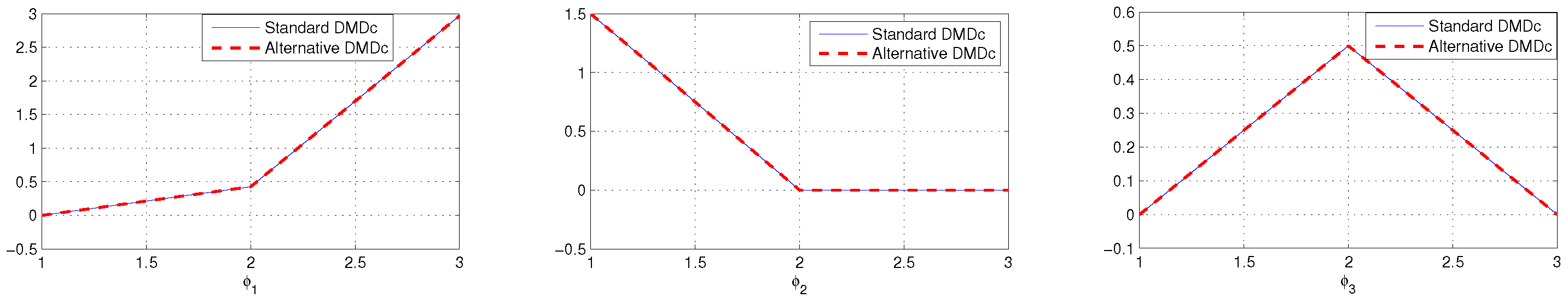
Example 2.

Nonlinear system with inputs.

Next, we consider a nonlinear dynamical system with external input:

$$\begin{array}{cc}\hfill {\dot{x}}_1& =\mu x_1,\hfill \\ \hfill {\dot{x}}_2& =\lambda (x_2-x_1^2)+\delta u,\hfill \end{array}$$

(33)

where $\lambda =-0.5$, $\mu =1.5$, and $\delta =1$, following examples in [14,24,25,26].

To enable a Koopman-based analysis, we augment the state with a nonlinear observable:

$$\mathbf{y}=\left[\begin{array}{c}{y}_1\\ y_2\\ y_3\end{array}\right]=\left[\begin{array}{c}{x}_1\\ x_2\\ x_1^2\end{array}\right].$$

The system is as follows:

$$\dot{\mathbf{y}}=\left[\begin{array}{ccc}\mu & 0& 0\\ 0& \lambda & -\lambda \\ 0& 0& 2\mu \end{array}\right] \mathbf{y}+\left[\begin{array}{c}0\\ \delta \\ 0\end{array}\right] u.$$

(34)

We collect measurements of the observables over 10 iterations, starting from the initial condition ${\left[234\right]}^T$. The input u consists of random signals sampled from a uniform distribution. The following matrices are constructed from the first five time snapshots:

$$X=\left[\begin{array}{ccccc}2& 3& 4.5& 6.75& 10.125\\ 3& 0.745& 5.697& 14.542& 45.506\\ 4& 12& 36& 108& 324\end{array}\right],\Gamma =\left[\begin{array}{ccccc}0.245& 0.07& -0.608& -1.222& 0.316\end{array}\right],$$

$$Y=\left[\begin{array}{ccccc}3& 4.5& 6.75& 10.125& 15.1875\\ 0.745& 5.697& 14.542& 45.506& 139.563\\ 12& 36& 108& 324& 972\end{array}\right].$$

Both algorithms yield the same DMD modes (see Figure 2) corresponding to the eigenvalues ${\lambda }_1=1.5$, ${\lambda }_2=-0.5$, and ${\lambda }_3=3$.

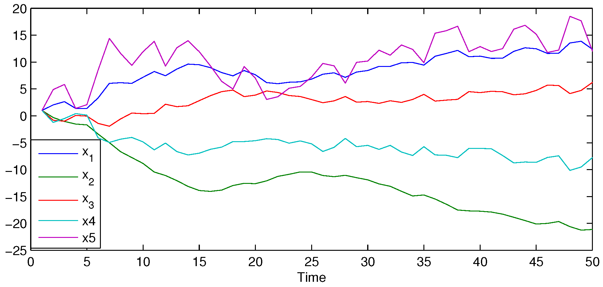
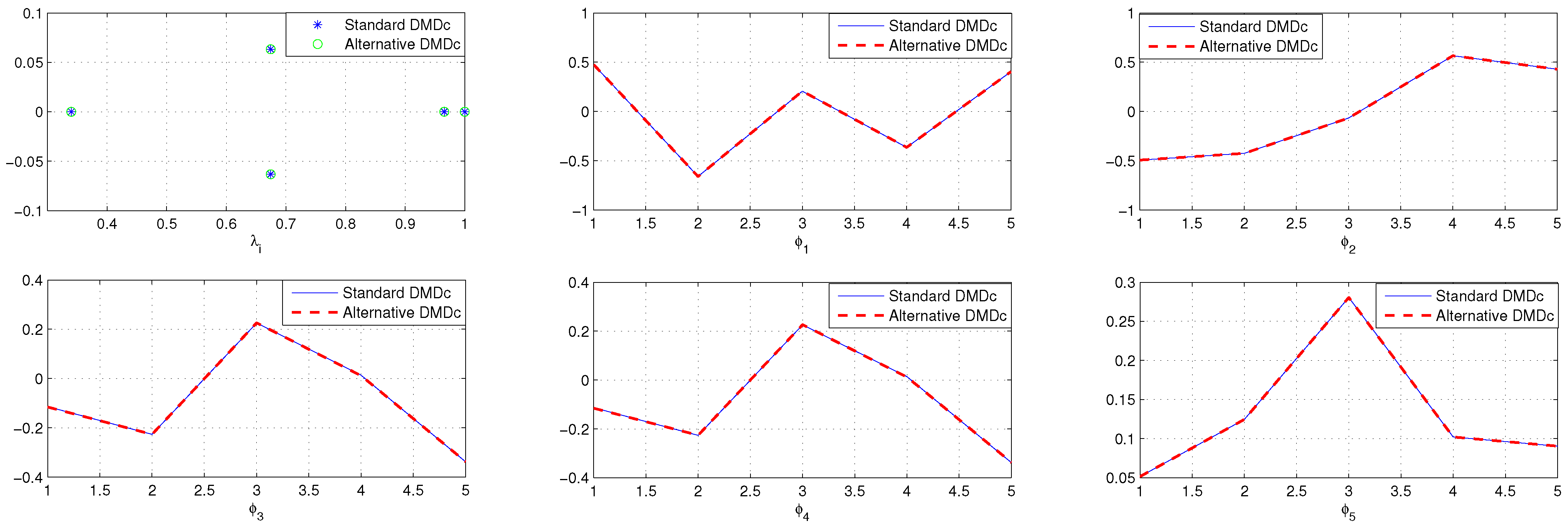
Example 3.

Large-scale stable linear systems.

Finally, we examine a large-scale linear system where the number of measurements significantly exceeds the dimensionality of the underlying dynamics.

The system exhibits a low-dimensional attractor. We construct a discrete-time linear state-space model using MATLAB’s drss function. The configuration includes:

• State dimension: 5
• Input dimension: 2
• Output dimension: 50

This yields matrices $A\in {\mathbb{R}}^{5\times 5}$, $B\in {\mathbb{R}}^{5\times 2}$, $C\in {\mathbb{R}}^{50\times 5}$, and $D\in {\mathbb{R}}^{50\times 2}$. The input sequence $\Gamma$ is generated via MATLAB’s randn function. The initial state is set as $x_0={[1,1,1,1,1]}^T$. Using these, we compute the data matrices X and Y, whose dynamics are shown in Figure 3.

The DMD modes and eigenvalues computed using both algorithms are displayed in Figure 4.

The results show complete agreement between the classical and alternative algorithms in both computed eigenvalues and DMD modes across all examples.

4. Conclusions

In this paper, we proposed an alternative formulation of the dynamic mode decomposition with control (DMDc), based on a structured low-rank approximation of the data matrices. We introduced and analyzed a new algorithm (Algorithm 2), which is shown to be more computationally efficient in terms of resource usage compared to the standard approach. Unlike traditional DMDc, this method constructs a reduced-order model using the singular value decomposition (SVD) of a block matrix, ${\mathrm{\Omega }}_1$. This allows for the direct computation of the reduced dynamics $\tilde{A}$ and control matrix $\tilde{B}$ without requiring a full SVD of the output matrix Y. Theoretical analysis has shown that all nonzero eigenvalues of the original system matrix A are captured by the eigenvalues of $\tilde{A}$, and a precise transformation allows recovery of the corresponding DMD modes.

The proposed algorithm simplifies the computational pathway by decoupling the effects of state and control inputs during model identification. This decoupling eliminates the need for certain matrix inversions and complex operator approximations inherent in traditional DMDc methods. As a result, it reduces memory usage and minimizes matrix multiplications. These features make the method particularly advantageous for large-scale systems, streaming data environments, and real-time control applications, where both computational speed and resource efficiency are critical. A comparison of matrix operations shows that Algorithm 2 requires storing fewer matrices and performing fewer multiplications than the standard approach, all while maintaining accuracy. Numerical examples have confirmed that the proposed method yields results identical to those obtained from the standard DMDc algorithm. Overall, the proposed method provides a practical, computationally efficient, and theoretically sound alternative to standard DMDc. Its modular structure and minimal resource footprint make it a promising tool for data-driven modeling and control in high-dimensional or rapidly changing environments.

However, despite its computational advantages, the proposed approach has certain limitations. One important feature of the formulation is that modes associated with zero eigenvalues are naturally excluded through the projection mechanism, which can enhance numerical robustness by focusing the model on the most dynamically significant behaviors. While this exclusion is often beneficial, it may be problematic in systems where zero dynamics have physical significance or are essential for stability analysis. In such cases, the method might overlook important behaviors. Additionally, the algorithm assumes that the data matrices are sufficiently rank-deficient and well-conditioned, which may not be the case in the presence of high noise levels or missing data.

Future work could focus on addressing these limitations by integrating regularization techniques, robust estimation strategies, and methods for explicitly capturing zero dynamics when necessary. Furthermore, extending the algorithm to work within adaptive or streaming frameworks for online learning and control would be a valuable direction, particularly for real-time applications in large-scale systems or robotics.