Applications of Shapley Value to Financial Decision-Making and Risk Management

Abstract

We investigate the application of the Shapley value in addressing risk-related challenges, focusing on two primary areas. The first area explores the role of the Shapley value in the financial sector, specifically in managing portfolio risk. By conceptualizing a portfolio of assets as a cooperative game, we analyze the contribution of individual securities to the reduction in overall portfolio risk. The second area addresses emergency facility logistics, where the Shapley value is utilized to optimize the selection of potential facility locations and mitigate the risks associated with the storage and transportation of hazardous materials. Using Markowitz’s mean-variance framework, the Shapley value facilitates a fair and efficient allocation of risk across portfolio assets, identifying both risk-increasing and risk-reducing assets. Through numerical experiments, we demonstrate that the Shapley value offers valuable insights into the equitable distribution of financial resources and the strategic placement of facilities to manage systemic risks. These findings highlight the practical advantages of integrating game-theoretic approaches into risk management strategies to enhance fairness, efficiency, and the robustness of decision-making processes.

1. Introduction

1.1. Background and Overview

Risk management is a fundamental challenge that requires innovative strategies to mitigate potential threats and uncertainties. This challenge is heightened by the constantly evolving economic environment and the unpredictability of financial markets [1,2,3]. Modern approaches are essential to effectively manage these risks, particularly in light of their increasing complexity.

Cooperative game theory, specifically the Shapley value, provides a systematic framework for addressing these issues by promoting equitable risk allocation and collaborative decision-making. Despite its theoretical promise, there is still a significant gap in translating cooperative game theory, particularly the Shapley value, into practical, workable techniques for real-world risk management. In areas such as financial portfolios and emergency logistics, where asymmetric contributions and cooperative incentives are crucial, existing methods often fail to methodically incorporate efficiency and fairness into risk or benefit allocation between participating entities, resulting in inefficiencies, disputes, or suboptimal outcomes. Motivated by these issues, our study suggests using the Shapley value from cooperative game theory to develop equitable, transparent, and mathematically sound risk attribution methodologies in portfolio management, as well as optimizing emergency facility placement. Our study aims to integrate the theoretical foundations of cooperative game theory with real-world risk management techniques by addressing fairness and decision accountability gaps, providing a robust methodology for enhancing choice quality in the face of uncertainty.

The Shapley value, introduced by Lloyd Shapley in 1953 [4], is one of the single-valued solution concepts for coalitional games to answer the question, “How will the gains or costs be distributed among players participating in a game if a coalition is formed?”, and has emerged as a cornerstone in understanding efficient and fair distribution within cooperative space. In other words, the answer to that question primarily depends on the player’s expectations before entering the game.

The application of the Shapley value to risk management has proven valuable in mitigating and managing potential risks. By providing a systematic method for the fair allocation of risks and benefits among coalition members based on their individual contributions, the Shapley value ensures that no member is unfairly burdened or rewarded. This equitable allocation is crucial in addressing complex risk-related problems, enabling more balanced and effective management of uncertainties and decision-making processes. Over time, the Shapley value has evolved beyond its theoretical roots, finding practical applications in fields such as political science, economics, and, notably, risk management. For instance, it has been used to analyze banks’ systemic importance [5], address the airport cost-sharing problem [6], and solve production planning challenges [7]. However, its full potential in addressing modern risk management issues, such as portfolio diversification and hazardous material logistics, remains underexplored.

Our study focuses on two key areas where Shapley value application can lead to more robust decision-making. The first area pertains to the financial sector, where we examine how risk can be managed in portfolio optimization. Specifically, we model a portfolio of assets as a cooperative game, where the securities in the portfolio aim to reduce the overall portfolio risk. The Shapley value allows investors to determine the exact contribution of each risky asset to the overall portfolio risk. The second area addresses emergency facility logistics, where we apply the Shapley value to a gradual coverage game to optimize the coverage of potential locations and minimize the risks associated with the storage and transportation of hazardous materials.

1.2. Literature Review

Managing risk and ensuring fair decision-making have become critical challenges in today’s financial and operational environments. While traditional risk management strategies such as diversification and hedging are commonly employed, they often lack transparency in the allocation of responsibilities and rewards to stakeholders. This gap has led researchers to explore cooperative game theory, particularly the Shapley value, as a framework for equitable and systematic resource and risk allocation.

The axiomatic fairness properties of the Shapley value, introduced by Shapley in 1953 [4], have made it a cornerstone of cooperative game theory. Over the years, its application has expanded significantly, particularly in the fields of finance, banking and logistics. In finance, Dhule et al. [8] utilized explainable machine learning algorithms combined with Shapley values to optimize retirement portfolio allocations, emphasizing risk transparency in decision-making. Similarly, Shapley value models have been employed to assess systemic risk among financial institutions, thereby enhancing macroprudential regulatory frameworks [5]. Traditionally, Markowitz’s mean-variance (MV) approach [1] has served as the foundation for portfolio optimization. However, the MV model does not account for the fair contribution of each asset to the overall portfolio risk.

Beyond finance, the Shapley value has found innovative applications in various fields. Zhou et al. [9] proposed a modified Shapley value method to optimize revenue distribution in agricultural e-commerce supply chains. Similarly, Liu et al. [10] applied modified Shapley models with fuzzy numbers to enhance logistics network optimization under uncertainty, demonstrating how both risk and logistical efficiency can be modeled simultaneously.

Adland et al. [11] employed Shapley value analysis to examine the interconnections among risk factors in marine logistics and transportation safety, using marine insurance claims data. In a similar vein, Yang et al. [12] utilized Shapley values to identify critical elements in freight-related incidents, focusing on their impact on logistics terminal design.

These studies collectively highlight the significant advantages of applying Shapley value approaches in both financial decision-making and operational logistics, fostering more equitable, transparent, and data-driven risk management strategies. Our study builds upon and expands prior research by systematically applying Shapley value techniques across these two domains, addressing the persistent challenge of equitable risk allocation in complex systems.

The remainder of this paper is structured as follows. In Section 2, we introduce the concepts of mean-variance analysis and Shapley value theory. Section 3 explores the Shapley value within the context of the coverage game and gradual coverage game. Section 4 presents applications in portfolio management and the gradual coverage game. In Section 5, we discuss the results of our analysis. Finally, Section 6 concludes the study with observations and suggests potential directions for future research.

2. Shapley Value for Portfolio Management

2.1. Shapley Value

In 1953, Lloyd Shapley introduced the Shapley value, a single-valued solution concept for coalitional games, with the goal of determining a fair and just method for distributing gains or costs among players in a cooperative game. In such games, each player contributes to the coalition’s overall success, and the Shapley value seeks to allocate rewards or penalties based on each player’s contribution. The value takes into account every possible combination of participants to determine the average marginal contribution of each player across all possible coalition formation orders. Essentially, the Shapley value evaluates each player’s relevance by comparing the impact of their participation in a coalition on the outcome relative to other possible formations of the coalition. This section draws on the foundational works of cooperative game theory [13,14,15].

Definition 1

([13]). Let $(\mathcal{N},v)$ be a coalitional game and $\sigma \in \pi \left(\mathcal{N}\right).$ The i-th coordinate corresponds to the marginal contribution vector $m^{\sigma }(\mathcal{N},v)\in {\mathbb{R}}^n$ about σ for all $i\in \mathcal{N}$ and is defined as

$$\begin{array}{c}\hfill m_i^{\sigma }(\mathcal{N},v)=v(P_i\left(\sigma \right)\cup \left\{i\right\})-v\left(P_i\left(\sigma \right)\right).\end{array}$$

(1)

Definition 2

([13]). The Shapley value $\varphi (\mathcal{N},v)$ of a coalitional game $(\mathcal{N},v)$ is the average of the marginal vectors of the game given by the formula

$$\begin{array}{c}\hfill \varphi (\mathcal{N},v)={\displaystyle \frac{1}{n!}}\sum _{\sigma \in \pi \left(\mathcal{N}\right)}{m}^{\sigma }(\mathcal{N},v).\end{array}$$

(2)

Then, ${\varphi }_i(\mathcal{N},v)$ is called the Shapley value of player i in game $(\mathcal{N},v)$ according to $\varphi .$

Using Definition 1, the Formula (2) can be rewritten as

$${\varphi }_i(\mathcal{N},v)={\displaystyle \frac{1}{n!}}\sum _{\sigma \in \pi \left(\mathcal{N}\right)}(v(P_i\left(\sigma \right)\cup \left\{i\right\})-v\left(P_i\left(\sigma \right)\right)).$$

(3)

Suppose i is a player and S is an arbitrary coalition that excludes player i. How many permutations of $\sigma$ exist such that $P_i\left(\sigma \right)=S$? For $P_i\left(\sigma \right)$ to be equal S, the players in S must enter the room before the player i under the permutation $\sigma$, followed by the player i, with the remaining players in $\mathcal{N}\setminus (S\cup \{i\left\}\right)$ entering afterward. The number of possible orderings for the players in S is $\left|S\right|!$, and the number of orderings for the players in $\mathcal{N}\setminus (S\cup \{i\left\}\right)$ is $\left(\right|\mathcal{N}|-|S|-1)!$. As a result, the total number of permutations of $\sigma$ under which $P_i\left(\sigma \right)=S$ is $\left|S\right|!\times \left(\right|\mathcal{N}|-|S|-1)!$. This leads to the conclusion that the Shapley value of a player i can be computed as follows [13]:

$$\begin{array}{c}\hfill {\varphi }_i(\mathcal{N},v)=\sum _{S\subseteq \mathcal{N}\setminus \left\{i\right\}}{\displaystyle \frac{\left|S\right|!\left(n-\left|S\right|-1\right)!}{n!}}\left(v\left(S\cup \left\{i\right\}\right)-v\left(S\right)\right)\end{array}$$

(4)

or

$$\begin{array}{c}\hfill {\varphi }_i(\mathcal{N},v)=\sum _{i\in S\subseteq \mathcal{N}}{\displaystyle \frac{\left(|S\right|-1)!\left(n-\left|S\right|\right)!}{n!}}\left(v\left(S\right)-v\left(S\setminus \left\{i\right\}\right)\right).\end{array}$$

(5)

Note that $\left|\mathcal{N}\right|=n$ and $\left|S\right|$ is the number of players in a coalition S, also ${\displaystyle \frac{\left|S\right|!(n-|S|-1)!}{n!}}={\displaystyle \frac{1}{n}}{\left(\begin{array}{c}n-1\\ \left|S\right|\end{array}\right)}^{-1}$.

The solution concept proposed by Shapley satisfies several properties that enable a fair division of profits among players in a coalition, assuming a grand coalition is formed. According to [13], the Shapley value satisfies additivity, anonymity, the dummy player property, and efficiency.

While the Shapley value provides a theoretically sound method for fair allocation, its practical computation becomes increasingly difficult as the number of players grows. Calculating the accurate Shapley value requires analyzing each player’s marginal contribution across all possible coalitions, leading to a computational complexity that increases exponentially with the number of participants (specifically, $2^n$ coalitions for n players). To address this issue, several approximation techniques [16,17,18,19,20] have been developed to estimate the Shapley value. Monte Carlo sampling techniques, in particular, provide high-quality approximations with significantly lower processing costs by randomly selecting a subset of coalitions and averaging the marginal contributions to approximate the Shapley value [19,20].

2.2. Mean-Variance Analysis

In 1952, Harry Markowitz introduced the Markowitz mean-variance (MV) model [1], a fundamental concept in modern portfolio theory and asset pricing theory [3]. The model is a portfolio optimization method that evaluates various portfolios composed of given securities and selects an efficient portfolio. An efficient portfolio is defined as one that offers the lowest level of risk (variance) for a given expected return (mean) or the highest expected return for a given level of risk. The MV model assumes that investors are rational and risk-averse, meaning they aim either to maximize the expected return of their portfolio for a given level of risk or to minimize their risk for a given expected return. However, for the purposes of this discussion, we will focus solely on risk minimization. The concepts presented in this section are based on the works of Markowitz [1], Samuelson [2], KOLM [3], and Huang [21].

2.2.1. Mathematical Formulation

Let n denote the number of risky assets in a portfolio with returns r assumed to be linearly independent. Here, r represents an n-dimensional random vector. Let 1 be an n-dimensional vector of ones, and let $\mu$ be an $n\times 1$ vector of the expected returns for each asset in the portfolio.

$$E\left[r\right]=\mu =\left(\begin{array}{c}{\mu }_1\\ ⋮\\ {\mu }_n\end{array}\right).$$

Let $\Sigma$ denote the $n\times n$ variance–covariance matrix of asset returns, which is a non-singular matrix:

$$\Sigma =Cov\left[r\right]=\left(\begin{array}{ccc}{\Sigma }_{11}& \dots & {\Sigma }_{1n}\\ ⋮& \ddots & ⋮\\ {\Sigma }_{n1}& \dots & {\Sigma }_{nn}\end{array}\right).$$

Let $\sigma$ denote an $n\times 1$ vector of asset volatilities (standard deviations), which corresponds to the square root of the diagonal elements of the variance–covariance matrix. Let w be an $n\times 1$ vector of portfolio weights, such that ${\sum }_{i=1}^n{w}_i=1$, where $w_i$ represents the weight of each asset i, i.e., the fraction of portfolio wealth allocated to asset i.

Portfolio Return: $r_p=w^{T}r={\sum }_{i=1}^n{w}_i{r}_i$ with

$${\mu }_p=E\left[r_p\right]=w^T\mu$$

$${\sigma }_p^2=var\left[r_p\right]=w^T\Sigma w$$

We assume that the predicted returns of at least two risky assets differ. Additionally, we allow for short sales, meaning that we permit assets to have negative weights. Short selling, or “shorting”, is an investment technique in which the seller sells a product (such as a stock, bond, or commodity) that they do not own. The seller borrows the security from a broker or another investor, sells it at the current market price, and later repurchases it at a lower price to repay the lender. A frontier portfolio is one that lies on the efficient frontier, which represents the optimal risky portfolio. The efficient frontier, also known as the portfolio frontier, shows the highest expected return for a given level of risk (measured by volatility or standard deviation) and the lowest risk for a given expected return.

To determine the portfolio weight w for a target mean return ${\mu }_0$, we consider the following optimization problem:

$$\begin{array}{c}\hfill \mathrm{Minimize}:{\displaystyle \frac{1}{2}}{w}^T\Sigma w\\ \hfill \mathrm{subject}\mathrm{to}:w^T\mathbf{1}& =1\hfill \\ \hfill w^T\mu & ={\mu }_0\hfill \end{array}$$

(6)

Using the Lagrange Multipliers approach [21], define the Lagrangian,

$$L(w,{\lambda }_1,{\lambda }_2)={\displaystyle \frac{1}{2}}{w}^T\Sigma w-{\lambda }_1(w^T\mathbf{1}-1)-{\lambda }_2(w^T\mu -{\mu }_0),$$

(7)

where ${\lambda }_1$ and ${\lambda }_2$ are positive constants. Calculate the first-order criteria

$${\displaystyle \frac{\partial L}{\partial w}}=\Sigma w-{\lambda }_1\mathbf{1}-{\lambda }_2\mu =\mathbf{0}$$

(8)

$${\displaystyle \frac{\partial L}{\partial {\lambda }_1}}=1-w^T\mathbf{1}=0$$

(9)

$${\displaystyle \frac{\partial L}{\partial {\lambda }_2}}={\mu }_0-w^T\mu =0,$$

(10)

where $\mathbf{0}$ is an n vector of zeros. Since $\Sigma$ is a positive definite matrix, the first-order criteria are necessary and sufficient for a global optimal solution. Solving for w in terms of ${\lambda }_1,{\lambda }_2$, using (8), we have

$${\Sigma }^{-1}\Sigma w-{\Sigma }^{-1}{\lambda }_1\mathbf{1}-{\Sigma }^{-1}{\lambda }_2\mu =0$$

$$w={\lambda }_1{\Sigma }^{-1}\mathbf{1}+{\lambda }_2{\Sigma }^{-1}\mu .$$

(11)

Substituting (11) into (9) and (10), we have

$$\begin{array}{cc}\hfill 1-w^T\mathbf{1}& =0\hfill \end{array}$$

$${\lambda }_1{\mathbf{1}}^T{\Sigma }^{-1}\mathbf{1}+{\lambda }_2{\mu }^T{\Sigma }^{-1}\mathbf{1}=1$$

(12)

and

$$\begin{array}{cc}\hfill {\mu }_0-w^T\mu & =0\hfill \end{array}$$

$${\lambda }_1{\mathbf{1}}^T{\Sigma }^{-1}\mu +{\lambda }_2{\mu }^T{\Sigma }^{-1}\mu ={\mu }_0.$$

(13)

Therefore, (12) and (13) in matrix form are

$$\begin{array}{c}\hfill \left(\begin{array}{cc}{\mathbf{1}}^T{\Sigma }^{-1}\mathbf{1}& {\mu }^T{\Sigma }^{-1}\mathbf{1}\\ {\mu }^T{\Sigma }^{-1}\mathbf{1}& {\mu }^T{\Sigma }^{-1}\mu \end{array}\right)\left(\begin{array}{c}{\lambda }_1\\ {\lambda }_2\end{array}\right)=\left(\begin{array}{c}1\\ {\mu }_0\end{array}\right).\end{array}$$

Let $a={\mathbf{1}}^T{\Sigma }^{-1}\mathbf{1},b={\mu }^T{\Sigma }^{-1}\mathbf{1}$, $d={\mu }^T{\Sigma }^{-1}\mu$ and $D=ad-b^2$, then

$$\begin{array}{c}\hfill \left(\begin{array}{cc}a& b\\ b& d\end{array}\right)\left(\begin{array}{c}{\lambda }_1\\ {\lambda }_2\end{array}\right)=\left(\begin{array}{c}1\\ {\mu }_0\end{array}\right).\end{array}$$

(14)

Since the inverse of a positive definite matrix is positive definite, $d>0$ and $a>0$. We claim that $D>0$. To show this, note that

$${(b\mu -d\mathbf{1})}^T{\Sigma }^{-1}(b\mu -d\mathbf{1})=d(ad-b^2).$$

Since ${\Sigma }^{-1}$ is positive definite, the left-hand side of the above equation is strictly positive. Hence, the right-hand side is strictly positive. From the fact that $d>0$, we have $ad-b^2>0$, or, equivalently, $D>0$. By solving (14), we obtain

$$\begin{array}{c}\hfill \left(\begin{array}{c}{\lambda }_1\\ {\lambda }_2\end{array}\right)={\left(\begin{array}{cc}a& b\\ b& d\end{array}\right)}^{-1}\left(\begin{array}{c}1\\ {\mu }_0\end{array}\right)\end{array}$$

(15)

$$\begin{array}{cc}\hfill & ={\displaystyle \frac{1}{ad-b^2}}\left(\begin{array}{c}d-b{\mu }_0\\ -b+a{\mu }_0\end{array}\right).\hfill \end{array}$$

Since $D=ad-b^2$, then

$$\begin{array}{c}\hfill \left(\begin{array}{c}{\lambda }_1\\ {\lambda }_2\end{array}\right)={\displaystyle \frac{1}{D}}\left(\begin{array}{c}d-b{\mu }_0\\ -b+a{\mu }_0\end{array}\right).\end{array}$$

(16)

Substitute ${\lambda }_1$ and ${\lambda }_2$ into (11) to obtain

$$\begin{array}{cc}\hfill w& ={\displaystyle \frac{1}{D}}(d-b{\mu }_0){\Sigma }^{-1}\mathbf{1}+{\displaystyle \frac{1}{D}}(a{\mu }_0-b){\Sigma }^{-1}\mu \hfill \end{array}$$

$$={\displaystyle \frac{1}{D}}(d{\Sigma }^{-1}\mathbf{1}-b{\Sigma }^{-1}\mu )+{\displaystyle \frac{{\mu }_0}{D}}(a{\Sigma }^{-1}\mu -b{\Sigma }^{-1}\mathbf{1})$$

(17)

Note that (17) gives the unique set of portfolio weights for the frontier portfolio with a given expected rate of return ${\mu }_o$:

$$w=x+y{\mu }_0$$

(18)

where

$$x={\displaystyle \frac{1}{D}}(d{\Sigma }^{-1}\mathbf{1}-b{\Sigma }^{-1}\mu$$

(19)

and

$$y={\displaystyle \frac{1}{D}}(a{\Sigma }^{-1}\mu -b{\Sigma }^{-1}\mathbf{1}).$$

(20)

Thus, the optimal weights of the mean-variance efficient portfolios are represented as a linear function of the given level of the expected return of the portfolio, ${\mu }_0$. Note that the frontier portfolio (18) has the expected return equal to ${\mu }_0$; that is,

$$w^T\mu ={\mu }_0.$$

Note that any portfolio that can be denoted by (18) is a frontier portfolio. The set of all frontier portfolios is called the portfolio frontier.

2.2.2. Variance of Optimal Portfolio with Return ${\mu }_0$

We need to calculate the variance for the optimal weight. From the solution portfolio (17),

$$w={\lambda }_1{\Sigma }^{-1}\mathbf{1}+{\lambda }_2{\Sigma }^{-1}\mu$$

has a minimum variance equal to

$$\begin{array}{cc}\hfill {\sigma }_0^2& =w^T\Sigma w\hfill \end{array}$$

(21)

$$\begin{array}{cc}\hfill {\sigma }_0^2& ={({\lambda }_1{\Sigma }^{-1}\mathbf{1}+{\lambda }_2{\Sigma }^{-1}\mu )}^T\Sigma ({\lambda }_1{\Sigma }^{-1}\mathbf{1}+{\lambda }_2{\Sigma }^{-1}\mu )\hfill \\ \hfill & ={\lambda }_1^2{\mathbf{1}}^T{\Sigma }^{-1}\mathbf{1}+2{\lambda }_1{\lambda }_2{\mathbf{1}}^T{\Sigma }^{-1}\mu +{\lambda }_2^2{\mu }^T{\Sigma }^{-1}\mu .\hfill \end{array}$$

Transform to a matrix form

$$\begin{array}{cc}\hfill {\sigma }_0^2& ={\left(\begin{array}{c}{\lambda }_1\\ {\lambda }_2\end{array}\right)}^T\left(\begin{array}{cc}{\mathbf{1}}^T{\Sigma }^{-1}\mathbf{1}& {\mu }^T{\Sigma }^{-1}\mathbf{1}\\ {\mu }^T{\Sigma }^{-1}\mathbf{1}& {\mu }^T{\Sigma }^{-1}\mu \end{array}\right)\left(\begin{array}{c}{\lambda }_1\\ {\lambda }_2\end{array}\right).\hfill \end{array}$$

(22)

Let $a={\mathbf{1}}^T{\Sigma }^{-1}\mathbf{1},b={\mu }^T{\Sigma }^{-1}\mathbf{1}$ and $d={\mu }^T{\Sigma }^{-1}\mu$, then

$$\begin{array}{cc}\hfill {\sigma }_0^2& ={\left(\begin{array}{c}{\lambda }_1\\ {\lambda }_2\end{array}\right)}^T\left(\begin{array}{cc}a& b\\ b& d\end{array}\right)\left(\begin{array}{c}{\lambda }_1\\ {\lambda }_2\end{array}\right).\hfill \end{array}$$

(23)

Substitute (15) into (22):

$$\begin{array}{cc}\hfill {\sigma }_0^2& ={\left(\begin{array}{c}1\\ {\mu }_0\end{array}\right)}^T{\left(\begin{array}{cc}a& b\\ b& d\end{array}\right)}^{-1}\left(\begin{array}{cc}a& b\\ b& d\end{array}\right){\left(\begin{array}{cc}a& b\\ b& d\end{array}\right)}^{-1}\left(\begin{array}{c}1\\ {\mu }_0\end{array}\right)\hfill \\ \hfill & ={\displaystyle \frac{1}{ad-b^2}}{\left(\begin{array}{c}1\\ {\mu }_0\end{array}\right)}^T\left(\begin{array}{c}d-b{\mu }_0\\ -b+a{\mu }_0\end{array}\right)\hfill \\ \hfill & ={\displaystyle \frac{1}{ad-b^2}}(d-2b{\mu }_0+a{\mu }_0^2)\hfill \end{array}$$

$$\begin{array}{c}\hfill {\sigma }_0^2={\displaystyle \frac{1}{D}}(a{\mu }_0^2-2b{\mu }_0+d).\end{array}$$

(24)

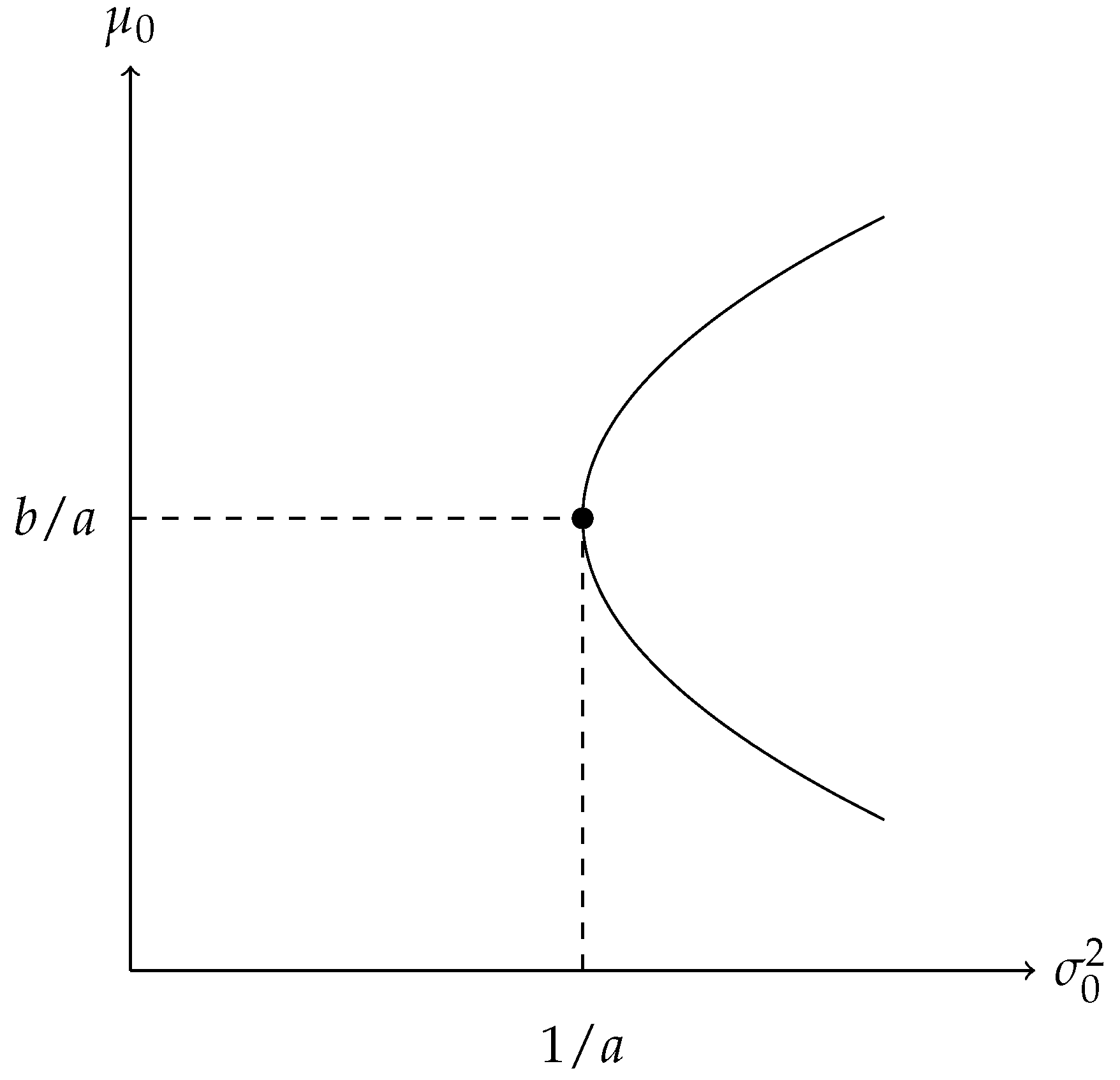
Equation (24) is a parabola in variance-expected rate of return space with vertex $({\displaystyle \frac{1}{a}},{\displaystyle \frac{b}{a}})$, as shown in Figure 1.

The parabolic curve is formed by assuming different values for parameter ${\mu }_p$. The global minimum variance portfolio (GMVP) can be obtained by setting

$${\displaystyle \frac{d{\sigma }_p^2}{d{\sigma }_p}}={\displaystyle \frac{1}{D}}(2a{\mu }_p-2b)=0,$$

so that ${\mu }_p={\displaystyle \frac{b}{a}}$ and ${\sigma }_p^2={\displaystyle \frac{1}{a}}.$ Correspondingly, from (16), ${\lambda }_1={\displaystyle \frac{1}{a}}$ and ${\lambda }_2=0$. Substituting the value of the GMVP ${\mu }_p$ and ${\sigma }_p^2$, the weight vector that gives the GMVP is given as

$$w={\displaystyle \frac{{\Sigma }^{-1}\mathbf{1}}{a}}={\displaystyle \frac{{\Sigma }^{-1}\mathbf{1}}{{\mathbf{1}}^T{\Sigma }^{-1}\mathbf{1}}}.$$

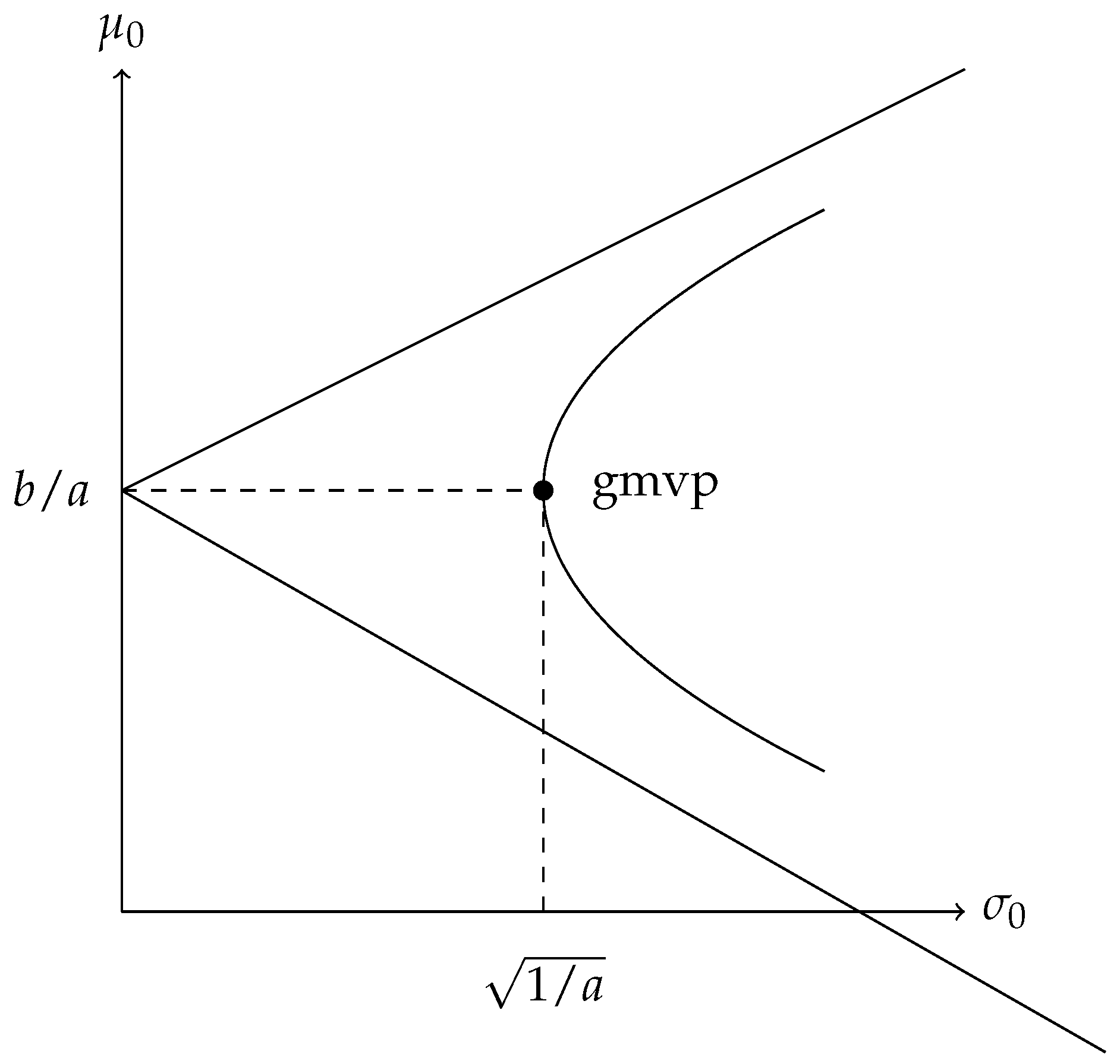
Equation (24) can equivalently be written as

$$\begin{array}{c}\hfill {\sigma }_0^2={\displaystyle \frac{a}{D}}{\left({\mu }_0-{\displaystyle \frac{b}{a}}\right)}^2+{\displaystyle \frac{1}{a}}\end{array}$$

(25)

which is a hyperbola in the standard deviation-expected rate of return space with center $(0,{\displaystyle \frac{b}{a}})$, as shown in Figure 2. From all the possible portfolios, the portfolio with the minimum variance is at $({\displaystyle \frac{1}{a}},{\displaystyle \frac{b}{a}})$.

2.2.3. Frontier Portfolios

Proposition 1

([21]). The entire portfolio frontier can be derived by forming portfolios of the two frontier portfolios x and $x+y.$

Proof. 

Choosing q arbitrarily as a frontier portfolio with an expected return ${\mu }_q$.

From (18), consider the following portfolio weights on x (19) and y (20): {$1-{\mu }_q,{\mu }_q$}, whose portfolio weights on risky assets are given as

$$(1-{\mu }_q)x+{\mu }_q(x+y)=x+y{\mu }_q=w_q.$$

That is, the portfolio {$1-{\mu }_q,{\mu }_q$} on x and $x+y$ produces the frontier portfolio q. Since q is chosen arbitrarily, we have shown that the entire portfolio frontier can be derived by two frontier portfolios x and $x+y$. □

Proposition 2

([21]). The portfolio frontier can be formed as a linear combination of any two frontier portfolios.

Proof. 

Let $p_1$ and $p_2$ be two distinct frontier portfolios. Since ${\mu }_{p_1}\ne {\mu }_{p_2}$, the expected returns on the two portfolios are not equal. Let q represent a frontier portfolio formed by these two frontier portfolios. Then, there exists a real number $\beta$ such that

$${\mu }_q=\beta {\mu }_{p_1}+(1-\beta ){\mu }_{p_2}$$

(26)

Consider a portfolio of $p_1$ and $p_2$ with weights $\beta$ and $(1-\beta )$, respectively. Since $p_1$ and $p_2$ are frontier portfolios, and from (26), then

$$\begin{array}{cc}\hfill \beta w_{p_1}+(1-\beta )w_{p_2}& =\beta (x+y{\mu }_{p_1})+(1-\beta )(x+y{\mu }_{p_2})\hfill \\ \hfill & =x+y{\mu }_q\hfill \\ \hfill & =w_q.\hfill \end{array}$$

(27)

Thus, a portfolio frontier can be formed by any two distinct frontier portfolios. □

3. Shapley Value for Coverage Game

Given the challenges associated with hazardous materials storage and transportation, it is crucial to discuss the importance of mitigating risks through the optimization of emergency facility locations. Based on [22], this section outlines a methodology that uses a gradual coverage game and the Shapley value to evaluate and select candidate sites for emergency facilities.

Consider the emergency facility placement problem for a certain region. Let us assume that the region is divided into m zones, denoted as $\mathbf{M}=\{1,2,\dots ,m\}$, and let $\tau \in {\mathbb{R}}_{+}^{\mathbf{M}}$ represent the emergency demand vector for each zone. To locate an emergency facility, we choose n zones, where $n\le m$. Therefore, $\mathbf{N}=\{1,2,\dots ,n\}$ represents the set of potential facility locations. If a location $i\in \mathbf{N}$ can serve a zone $j\in \mathbf{M}$ within a predetermined timeframe, then the location i covers zone j. The coverage matrix is denoted as $\mathcal{C}=\left(c_{ij}\right)\in {\mathbb{R}}^{n\times m}$, where

$$c_{ij}=\left\{\begin{array}{cc}1\hfill & \mathrm{if}\mathrm{an}\mathrm{emergency}\mathrm{facility}\mathrm{sited}\mathrm{in}\mathrm{zone}i\mathrm{covers}\mathrm{zone}j,\hfill \\ 0\hfill & \mathrm{otherwise}.\hfill \end{array}\right.$$

Thus, the emergency facility location problem can be represented by the tetrad $(\mathbf{N},\mathbf{M},\mathcal{C},\tau )$.

The coverage game $(\mathbf{N},v_c)$ defined in [23] is a special type of TU-game, where a coalition of prospective locations is valued based on the total demand it can satisfy. Specifically, the value of a coalition S is given by

$$v_c\left(S\right)=\sum _{i\in B_S}{\tau }_i\mathrm{for}\mathrm{all}S\subseteq \mathbf{N},$$

where $B_S=\{j\in \mathbf{M}\mid \exists i\in S,\mathrm{such}\mathrm{that}{c}_{ij}=1\}$ is the set of zones covered by at least one emergency unit in S. Each zone is assumed to be covered by one emergency unit. The set of all coverage games over $\mathbf{N}$ is denoted by $G_c^{\mathbf{N}}$.

The Shapley value was used in [23] to solve the coverage game because the relevance of a potential location is primarily based on its marginal contribution to the existing locations. As shown in [23], the Shapley value for the coverage game can be computed as

$${\varphi }_i(\mathbf{N},v_c)=\sum _{j\in B_{\left\{i\right\}}}{\displaystyle \frac{{\tau }_j}{{\sum }_{l\in \mathbf{N}}{c}_{lj}}},$$

(28)

This expression indicates that the importance of location $i\in \mathbf{N}$ is determined by how much demand it can satisfy, assuming the demand in each zone $j\in \mathbf{M}$ is equally divided across the areas it covers.

The coverage game $(\mathbf{N},v_c)$ can be represented as the summation of m zone games. That is, we have

$$v_c=\sum _{j\in \mathbf{M}}{v}_c^j,$$

where in the zone game about zones $j\in \mathbf{M}$, denoted $(\mathbf{N},v_c^j)$, the needs of other zones are ignored. Specifically, for every $S\subseteq \mathbf{N}$, the value of the coalition S in the zone j is given by

$$v_c^j\left(S\right)=\left\{\begin{array}{cc}{\tau }_j\hfill & \mathrm{if}j\in B_S,\hfill \\ 0\hfill & \mathrm{otherwise}.\hfill \end{array}\right.$$

3.1. Gradual Coverage Game

The classic coverage model assumes that an incident area is either “covered” by an emergency facility within a specific distance or “not covered at all”. However, when dealing with hazardous waste, the responsiveness of an emergency facility is inversely proportional to the response time. This creates significant risks for neighboring regions, as slower response times can result in larger-scale consequences. In [22], the authors propose a risk evaluation approach that considers the response time from the emergency facility to the incident’s location.

Let $\mathbf{N}$ and $\mathbf{M}$ represent the sets of potential locations for emergency facilities and incident sites, respectively. The partial coverage matrix can be defined as follows:

$$\begin{array}{c}\hfill c_{ij}=\left\{\begin{array}{cc}1\hfill & (T_{ij}\le R_l)\hfill \\ {\displaystyle \frac{R_u-T_{ij}}{R_u-R_l}}\hfill & (R_l<T_{ij}<R_u),\hfill \\ 0\hfill & (T_{ij}\ge R_u)\hfill \end{array}\right.\end{array}$$

(29)

where $T_{ij}$ denotes the response time from $i\in \mathbf{N}$ to $j\in \mathbf{M}$, and $R_l$ and $R_u$ represent the most and least desired response times, respectively. According to Equation (29), location j is fully covered by the facility i when the response time $T_{ij}$ is less than $R_l$, partially covered when $T_{ij}$ is between $R_l$ and $R_u$, and not covered at all when $T_{ij}$ exceeds $R_u$. The special case of Equation (29), where $R_l=R_u$, was studied in [23]. In this case, the coverage matrix $\mathcal{C}={\left\{c_{ij}\right\}}_{i\in \mathbf{N},j\in \mathbf{M}}$ is a 0–1 matrix.

Define ${\tau }_j$ as the highest risk at the incident site j, representing the population at risk. The risk of establishing a facility at a potential location i can then be calculated as

$${\mathcal{R}}_{ij}=(1-c_{ij}){\tau }_j.$$

(30)

When the site j is fully covered, the danger is minimized. However, when j is not covered, the risk increases significantly. The utility of employing facility i to respond to a site j is defined as the decrease in risk and is expressed as follows:

$${\mathcal{U}}_{ij}=c_{ij}{\tau }_j.$$

(31)

In a cooperative game with transferable utility, a gradual coverage game for hazardous materials $(\mathbf{N},v_{gc})$ was described in [22], where $\mathbf{N}$ represents the set of potential sites for emergency facilities, and $v_{gc}$ is the characteristic function, defined as

$$\begin{array}{c}\hfill v_{gc}\left(S\right)=\sum _{j\in B_S}\underset{i\in S}{max}{\mathcal{U}}_{ij}\forall S\subseteq \mathbf{N},\end{array}$$

(32)

where $B_S=\{j\in \mathbf{M}|\exists i\in S,\mathrm{s}.\mathrm{t}.c_{ij}>0\}$ is the set of incident locations that are at least partially covered by one facility located in S. Denote the set of all gradual coverage games over $\mathbf{N}$ by $G_{gc}^{\mathbf{N}}.$

This game aims to assess the decrease in system rescue risk through a coalition of locations. As stated in [22], at each incident site j, the utility is evaluated by the maximum risk reduction achieved by the nearest facility, denoted as $(\underset{i\in S}{max}{\mathcal{U}}_{ij})$, rather than by summing the utilities $\left({\sum }_{i\in S}{\mathcal{U}}_{ij}\right)$, since the risk reduction cannot be accumulated due to time constraints.

Moreover, if $R_l=R_u$, meaning there is no difference between the most and the least desired response times, then for every $j\in B_S$,

$$\underset{i\in S}{max}{\mathcal{U}}_{ij}=\underset{i\in S}{max}{c}_{ij}{\tau }_j={\tau }_j,$$

and consequently, $(\mathbf{N},v_{gc})=(\mathbf{N},v_c)$. Thus, we have $G_c^{\mathbf{N}}\subseteq G_{gc}^{\mathbf{N}}$.

3.2. Shapley Value of the Gradual Coverage Game

By using the Shapley value, the objective is to rank the potential locations by importance based on their marginal contributions to the total emergency response performance. The emergency system manager can use this sequence to prioritize the construction of facilities at specific locations. Note that if many players have the same Shapley value, a random tie-breaking rule may be employed.

As highlighted in [22], to determine the Shapley value of the gradual coverage game specified by Equation (32), define a j-th gradual zone game as an auxiliary game $(\mathbf{N},$$v_{gc}^j\in G^{\mathbf{N}})$ for each $j\in \mathbf{M}$, as follows:

$$v_{gc}^j\left(S\right)=\underset{i\in S}{max}{\mathcal{U}}_{ij}\mathrm{for}\mathrm{all}S\subseteq \mathbf{N}.$$

Notably, if the least and the most desired response times are equal, i.e., $R_l=R_u$, then the j-th zone game equals the j-th gradual zone game. Consequently, we have

$$v_{gc}\left(S\right)=\sum _{j\in B_S}\underset{i\in S}{max}{\mathcal{U}}_{ij}=\sum _{j\in \mathbf{M}}\underset{i\in S}{max}{\mathcal{U}}_{ij}=\sum _{j\in \mathbf{M}}{v}_{gc}^j\left(S\right),$$

where $\underset{i\in S}{max}{\mathcal{U}}_{ij}=0$ if $j\notin B_S$. Based on the additivity property of the Shapley value, we obtain the following decomposition:

$$\begin{array}{c}\hfill \varphi (\mathbf{N},v_{gc})=\sum _{j\in M}\varphi (\mathbf{N},v_{gc}^j).\end{array}$$

(33)

Equation (33) decomposes the Shapley value of the gradual coverage game into the sum of the Shapley values of the individual gradual zone games. To compute the Shapley value of each gradual zone game, we note that for each $j\in \mathbf{M}$, $(\mathbf{N},v_{gc}^j)$ corresponds to the generalized airport game model [24]. Furthermore, if the utility values satisfy

$$0={\mathcal{U}}_{0j}\le {\mathcal{U}}_{1j}\le \dots \le {\mathcal{U}}_{nj},$$

(34)

then $(\mathbf{N},v_{gc}^j)$ is an airport game [25]. According to [25], for each $i\in \mathbf{N}$, the Shapley value is given by

$${\varphi }_i(\mathbf{N},v_{gc}^j)=\sum _{l=1}^i{\displaystyle \frac{{\mathcal{U}}_{lj}-{\mathcal{U}}_{(l-1)j}}{n+1-l}}.$$

(35)

Thus, rather than calculating the Shapley value of $(\mathbf{N},v_{gc})$ directly from its definition, we can determine it using Equation (33), by rearranging the individual cover vector ${\mathcal{U}}_j=\{{\mathcal{U}}_{1j},{\mathcal{U}}_{2j},\dots ,{\mathcal{U}}_{nj}\}$ for each $j\in \mathbf{M}$, as shown in Equation (34).

Similarly, Equation (35) can be simplified as follows:

$$\varphi (\mathbf{N},v_{gc}^j)=\left\{\begin{array}{cc}{\displaystyle \frac{{\tau }_j}{{\sum }_{l=1}^n{c}_{lj}}}\hfill & \mathrm{if}j\in B_{\left\{i\right\}}\hfill \\ 0\hfill & \mathrm{otherwise},\hfill \end{array}\right.$$

(36)

This expression is precisely the j-th term of Equation (28).

As noted in [22], Equation (35) can be explained as follows. Equation (34) allows for a level-by-level distribution of utilities ${\left\{\mathcal{U}\right\}}_{l=0}^n$ among prospective sites. To distribute the portion ${\mathcal{U}}_{1j}-{\mathcal{U}}_{0j}$ evenly among all prospective sites, we assume that each location contributes equally. Notably, only some sites $2,3,\dots ,n$ contribute to the portion ${\mathcal{U}}_{2j}-{\mathcal{U}}_{1j}$, so this portion is divided evenly among those sites. This process continues for the remaining portions, with the part ${\mathcal{U}}_{nj}-{\mathcal{U}}_{(n-1)j}$ being distributed among all sites. After distributing these utilities, the location i receives its Shapley value.

4. Results

4.1. Application in Portfolio Management

In this section, we model a portfolio of 10 different assets using Markowitz’s mean-variance model [1,26,27] to determine the optimal asset weights that correspond to a high expected return and lower variance. The Shapley value is then employed to calculate the individual Shapley value for each asset. This ensures a fair distribution of risk among the assets (players) that make up the optimal mean-variance portfolio, such that each asset’s marginal contribution to the portfolio’s overall risk profile can be determined using the Shapley value, as given by Equation (4).

The objective is to construct portfolios with the lowest variance for the highest possible returns. Using Equation (25), we compute the frontier portfolios for a range of expected returns defined in the mean-variance space. The frontier portfolio with the lowest variance is the global minimum-variance portfolio.

Furthermore, we examine two specific cases:

(a)

The global minimum-variance portfolio (GMVP).

(b)

Portfolios for a given expected return.

To understand the application of the Shapley value and mean-variance analysis in the risk management of portfolio investments, we constructed a portfolio containing different types of assets using Yahoo Finance data [28]. The data consist of 2678 daily nominal returns from historical prices of three Polish stocks from the Warsaw Stock Exchange (WSE), three Italian stocks from Borsa Italiana, two commodity ETFs, and two bond ETFs from January 2014 to April 2024.

1.

Polish Stocks:

–

PKN.WA—PKN Orlen SA

–

PKO.WA—PKO Bank Polski SA

–

KGH.WA—KGHM Polska Miedź SA

2.

Italian Stocks:

–

ENI.MI—Eni SpA

–

ISP.MI—Intesa Sanpaolo SpA

–

AZM.MI—A2A SpA

3.

Commodities:

–

GLD—Gold (SPDR Gold Shares ETF)

–

SLV—Silver (iShares Silver Trust ETF)

4.

Bonds:

–

AGG—iShares Core U.S. Aggregate Bond ETF (representing the US bond market)

–

TLT—iShares 20+ Year Treasury Bond ETF (representing long-term US Treasury bonds)

The summary statistics are shown in

Table 1. Summary statistics of daily returns for each asset.

Asset	Count	Mean	Std	Min	25%	50%	75%	Max
AGG	2678	0.000059	0.003178	−0.040010	−0.001311	0.000091	0.001541	0.023721
AZZM.MI	2678	0.000551	0.020969	−0.158929	−0.009751	0.000682	0.011100	0.153716
ENI.MI	2678	0.000338	0.017202	−0.208521	−0.007812	0.000592	0.008811	0.149307
GLD	2678	0.000264	0.008722	−0.053694	−0.004422	0.000109	0.004820	0.049038
ISP.MI	2678	0.000689	0.020472	−0.229407	−0.009109	0.000427	0.010517	0.144455
HGH.WA	2678	0.000423	0.024315	−0.159864	−0.013485	0.000000	0.013688	0.116803
PKN.WA	2678	0.000530	0.020804	−0.096266	−0.011020	0.000000	0.011910	0.143943
PKO.WA	2678	0.000433	0.019647	−0.168209	−0.010257	0.000000	0.011148	0.132684
SLV	2678	0.000224	0.016009	−0.135926	−0.007389	0.000000	0.007829	0.091429
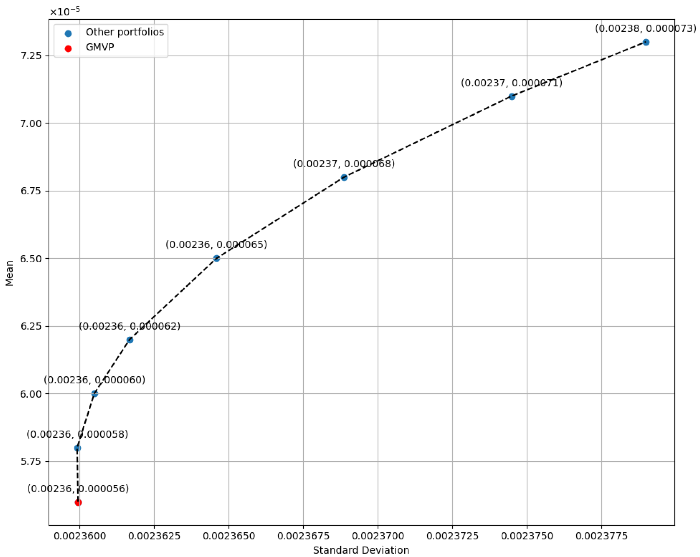
TLT	2678	0.000085	0.009308	−0.066683	−0.005403	0.000074	0.005446	0.075195

. Using the data from Yahoo Finance, we computed the means and the variance–covariance matrix. Assuming an allowance for short sales, the frontier of mean-variance (MV) optimal portfolios is obtained from Equation (25) for the expected returns presented in

Table 2. Statistics of MV frontier portfolio.

Portfolio	Expected Return (%)	Standard Deviation (%)
A	0.0056	0.2358
B	0.0058	0.2359
C	0.0060	0.2360
D	0.0062	0.2361
E	0.0065	0.2365
F	0.0068	0.2370
G	0.0071	0.2376
H	0.0073	0.2381

, and the results are illustrated in Figure 3.

According to Table 2, it is observed that for higher expected returns, the risk associated with the optimal portfolios increases. This result aligns with the expectations of the mean-variance (MV) portfolio theory, which posits that higher returns are generally accompanied by higher risk.

Table 3. Optimal asset weights for each MV frontier portfolio.

Portfolio	A	B	C	D	E	F	G	H
$\mathbf{\mu }$	0.000056	0.000058	0.000060	0.000062	0.000065	0.000068	0.000071	0.000073
Asset
AGG	1.3009	1.2559	1.2859	1.2784	1.2671	1.2559	1.2447	1.2334
AZM.MI	−0.0129	−0.0101	−0.0119	−0.0115	−0.0108	−0.0101	−0.0094	−0.0087
ENI.MI	−0.0100	−0.0119	−0.0107	−0.0110	−0.0115	−0.0120	−0.0125	−0.0130
GLD	0.0619	0.0905	0.0714	0.0762	0.0834	0.0906	0.0977	0.1049
ISP.MI	0.0096	0.0165	0.0119	0.0131	0.0148	0.0166	0.0183	0.0200
KGH.WA	−0.0023	−0.0022	−0.0023	−0.0023	−0.0023	−0.0022	−0.0022	−0.0022
PKN.WA	0.0049	0.0085	0.0061	0.0067	0.0076	0.0085	0.0094	0.0103
PKO.WA	0.0030	0.0038	0.0033	0.0034	0.0037	0.0039	0.0041	0.0043
SLV	−0.0414	−0.0504	−0.0444	−0.0459	−0.0482	−0.0504	−0.0527	−0.0549
TLT	−0.3136	0.3006	−0.3093	−0.3071	−0.3039	−0.3006	−0.2974	−0.2942

shows the optimal asset weights for portfolios along the portfolio frontier. These weights are computed using Equation (17) to minimize portfolio variance for a given expected return. Some of the weights are negative, indicating a short position in those assets.

4.1.1. Global Minimum-Variance Portfolio (GMVP)

The expected return of the GMVP is given by ${\displaystyle \frac{b}{a}}$ from Equation (24), and the variance of the GMVP is ${\displaystyle \frac{1}{a}}$, where $a={\mathbf{1}}^T{\Sigma }^{-1}\mathbf{1}$ and $b={\mu }^T{\Sigma }^{-1}\mathbf{1}$. This makes it easier to calculate the Shapley value for assets in the GMVP, as described in [27] and outlined below:

(1)

Determine all $2^{\mathcal{N}}$ subsets of assets in the set $\mathcal{N}$.

(2)

For each subset $S\subseteq \mathcal{N}$, compute the variance–covariance matrix ${\Sigma }_S$ and $a_S={\mathbf{1}}_S^T{\Sigma }_S^{-1}{\mathbf{1}}_S$.

(3)

To calculate the variance of the GMVP for each subset S, use the following formula:

$${\sigma }_{GMVP}^2\left(S\right)={\displaystyle \frac{1}{a_S}}.$$

(4)

Using Equation (4), the Shapley value for each asset i in the GMVP is computed as

$$\begin{array}{cc}\hfill {\varphi }_i\left({\sigma }_{GMVP}^2\right)& =\sum _{S\subseteq \mathcal{N}\setminus \left\{i\right\}}{\displaystyle \frac{\left|S\right|!\times (n-|S|-1)!}{n!}}\left({\sigma }_{GMVP}^2(S\cup \left\{i\right\})-{\sigma }_{GMVP}^2\left(S\right)\right)\hfill \\ \hfill & =\sum _{S\subseteq \mathcal{N}\setminus \left\{i\right\}}{\displaystyle \frac{\left|S\right|!\times (n-|S|-1)!}{n!}}\left({\displaystyle \frac{1}{a_{S\cup \left\{i\right\}}}}-{\displaystyle \frac{1}{a_S}}\right).\hfill \end{array}$$

(37)

(5)

Therefore, the sum of the Shapley values for all the assets in the GMVP is given by

$$\sum _{i=1}^n{\varphi }_i\left({\sigma }_{GMVP}^2\right)={\displaystyle \frac{1}{a_{\mathcal{N}}}}.$$

The Shapley values for the GMVP assets are calculated using Equation (37). These values are reported in

Table 4. Shapley value of each asset in GMVP.

Asset	GVMP Weights (%)	Shapley Value (%)	Relative SV (%)
AGG	130.09	−0.5378	−228.06
AZM.MI	−1.29	0.1744	73.97
ENI.MI	−1.00	0.1150	48.76
GLD	6.19	−0.1341	−56.87
ISP.MI	0.96	0.1679	71.19
KGH.WA	−0.23	0.2264	96.00
PKN.WA	0.49	0.1684	71.42
PKO.WA	0.30	0.1546	65.54
SLV	−4.14	0.0652	27.66
TLT	−31.36	−0.1642	−69.61

.

4.1.2. Portfolios for a Given Expected Return

For arbitrary expected returns, the Shapley value for the assets of all optimal mean-variance portfolios along the frontier can be developed. Since the variance of a frontier portfolio is determined by ${\sigma }^2=w^T\Sigma w$, the mean-variance efficient frontier depends on the given mean return ${\mu }_p$.

In this case, as shown in [27], the Shapley value is obtained as follows:

(1)

Determine all $2^{\mathcal{N}}$ subsets of assets in set $\mathcal{N}$.

(2)

For each subset $S\subseteq \mathcal{N}$, compute the variance–covariance matrix ${\Sigma }_S$ and the expected return vector ${\mu }_S$.

(3)

Define an arbitrary set of required mean returns ${\mu }_p>{\displaystyle \frac{b_S}{a_S}}$, where $a={\mathbf{1}}^T{\Sigma }^{-1}\mathbf{1}$ and $b={\mu }^T{\Sigma }^{-1}\mathbf{1}$ are the quadratic forms for the entire set $\mathcal{N}$. Use the equation ${\sigma }^2=w^T\Sigma w$ to calculate the frontier portfolio variance for each subset $S\cup \left\{i\right\}\subseteq \mathcal{N}$ and for all mean returns ${\mu }_p$.

(4)

Using Equation (4), the Shapley value for each asset i in an optimal frontier portfolio subject to a given expected return ${\mu }_p$ is calculated as

$$\begin{array}{cc}\hfill {\varphi }_i({\sigma }_p^2;{\mu }_p)& =\sum _{S\subseteq \mathcal{N}\setminus \left\{i\right\}}{\displaystyle \frac{\left|S\right|!\times (n-|S|-1)!}{n!}}({\sigma }_p^2({\mu }_p;S\cup \left\{i\right\})-{\sigma }_p^2({\mu }_p;S)).\hfill \end{array}$$

(38)

(5)

Therefore, for a given expected return ${\mu }_p$, the sum of the Shapley values for all the assets in the optimal frontier portfolio is

$$\sum _{i=1}^n{\varphi }_i({\sigma }_p^2;{\mu }_p)={\sigma }_p^2({\mu }_p;\mathcal{N}).$$

(39)

From Equation (38), given that efficient portfolios aim to minimize variance (risk) ${\sigma }_p^2$ for a given expected return (mean) ${\mu }_p$, the incremental risks $\left({\sigma }_p^2({\mu }_p;S\cup \left\{i\right\})-{\sigma }_p^2({\mu }_p;S)\right)$ are non-positive for any asset i and any set S that does not include i, as introduced by Samuelson [2].

Note that Table 3 depicts the optimal weight of each asset along the mean-variance efficient frontier for a given mean, calculated by minimizing portfolio variance. The Shapley values of portfolio assets on the MV frontier are computed using Equation (38) and are reported in

Table 5. Shapley value of each asset in MV frontier portfolios.

Portfolio	B	C	D	E	F	G	H
$\mathbf{\mu }$	0.000058	0.000060	0.000062	0.000065	0.000068	0.000071	0.000073
Asset	(%)	(%)	(%)	(%)	(%)	(%)	(%)
AGG	−1.4750	−1.4653	−1.4555	−1.4405	−1.4356	−1.4201	−1.4165
AZM.MI	0.7223	0.7200	0.7177	0.7141	0.7002	0.6966	0.6959
ENI.MI	−0.1718	−0.1718	−0.1719	−0.1720	−0.1825	−0.1827	−0.1810
GLD	−0.4089	−0.4088	−0.4087	−0.4087	−0.4192	−0.4193	−0.4178
ISP.MI	−0.2523	−0.2497	−0.2471	−0.2433	−0.2499	−0.2463	−0.2421
KGH.WA	1.2021	1.1954	1.1887	1.1786	1.1582	1.1482	1.1432
PKN.WA	0.8085	0.8057	0.8028	0.7985	0.7839	0.7795	0.7783
PKO.WA	1.1372	1.1309	1.1245	1.1150	1.0951	1.0856	1.0809
SLV	−0.3686	−0.3679	−0.3671	−0.3660	−0.3753	−0.3741	−0.3716
TLT	−0.9576	−0.9524	−0.9471	−0.9391	−0.8380	−0.8298	−0.8313
Total SV	0.2359	0.2360	0.2361	0.2365	0.2370	0.2376	0.2381

. Some assets have negative Shapley values, indicating that they contribute lower risk to the portfolio. This is often the case with AGG, ENI.MI, GLD, ISP.MI, SLV, and TLT. On the other hand, positive Shapley values indicate that these assets enhance the risk along the optimal frontier, contributing to higher mean returns. Portfolio managers may use this information to make strategic decisions regarding asset selection and allocation, balancing risk and return according to their investment goals.

4.2. Application in Gradual Coverage Game

The model is designed to generate a sequence of potential locations and rank them according to their significance in descending order. This approach helps individuals or organizations make well-informed decisions when selecting locations for emergency facilities. Below is the pseudocode for the model implementation.

The steps for the implementation are as follows:

(a)

Identify prospective facility locations, denoted as set $\mathbf{N}$.

(b)

Define $\mathbf{M}$ zones and associate each zone j with a vector ${\tau }_j$, reflecting the risk or emergency demand level for each zone.

(c)

Determine the response times $T_{ij}$ for each facility i to cover each zone j, and calculate the coverage matrix using Equation (29).

(d)

Calculate the risk ${\mathcal{R}}_{ij}$ associated with each zone j for each prospective facility location i using Equation (30), and the utility ${\mathcal{U}}_{ij}$ of placing a facility at each location using Equation (31).

(e)

For each zone j, sort the utilities ${\mathcal{U}}_j$ in ascending order as required.

(f)

Calculate the gradual Shapley values ${\varphi }_i(\mathbf{N},v_{gc}^j)$ (as in Equation (35)) for each location and its corresponding zone, using the sorted utilities, but return the results in the original utility order.

(g)

Sum the values across all zones for each location. This gives the total Shapley value for each location.

(h)

Rank the potential facility locations by their total Shapley values and allocate locations for facility placement to optimize coverage while minimizing risk.

This method ensures that prospective emergency facility locations are selected through a fair assessment of their contributions to total coverage, considering the varying levels of risk reduction provided by different zones. This aids in effective decision-making regarding emergency facility placement.

Furthermore, the Shapley value reflects each location’s contribution to the overall emergency response system. Due to the unavailability of real datasets, only a theoretical example of the application of these steps is presented below.

Let us consider a small city with 10 hazardous waste generation areas. We assume that $\mathbf{N}=\mathbf{M}$, meaning that all the zones are prospective areas for locating emergency facilities and that the risk or emergency demand levels are equal across all zones. The least and most desired response times are 10 and 30 min, respectively. We generate the response times for each facility location $i\in \mathbf{N}$ to cover a zone $j\in \mathbf{M}$ using a random number generator function in Python 3.9.6.

The generated times range between 5 and 35 min, as shown in

Table 6. Randomly generated response times across various zones and locations.

	Zone1	Zone2	Zone3	Zone4	Zone5	Zone6	Zone7	Zone8	Zone9	Zone10
Loc1	12	14	8	28	17	20	9	7	7	5
Loc2	17	22	34	14	30	29	6	12	21	22
Loc3	16	13	29	10	31	8	13	11	35	34
Loc4	5	31	25	30	13	30	13	11	10	14
Loc5	14	25	32	28	35	32	32	33	16	7
Loc6	32	24	15	26	17	21	12	10	12	20
Loc7	13	7	35	34	31	32	35	22	31	14
Loc8	5	34	14	23	27	33	14	32	29	21
Loc9	11	18	18	24	14	18	19	10	12	14
Loc10	13	31	30	6	7	6	19	25	13	21

. Below is the randomly generated emergency demand vector ${\tau }_j$:

$$\tau =[9,10,8,10,7,6,10,6,5,8].$$

We present partial calculations that help in obtaining the Shapley value for the prospective locations.

Table 7. Coverage matrix.

	Zone1	Zone2	Zone3	Zone4	Zone5	Zone6	Zone7	Zone8	Zone9	Zone10
Loc1	0.90	0.80	1.00	0.10	0.65	0.50	1.00	1.00	1.00	1.00
Loc2	0.65	0.40	0.00	0.80	0.00	0.05	1.00	0.90	0.45	0.40
Loc3	0.70	0.85	0.05	1.00	0.00	1.00	0.85	0.95	0.00	0.00
Loc4	1.00	0.00	0.25	0.00	0.85	0.00	0.85	0.95	1.00	0.80
Loc5	0.80	0.25	0.00	0.10	0.00	0.00	0.00	0.00	0.70	1.00
Loc6	0.00	0.30	0.75	0.20	0.65	0.45	0.90	1.00	0.90	0.50
Loc7	0.85	1.00	0.00	0.00	0.00	0.00	0.00	0.40	0.00	0.80
Loc8	1.00	0.00	0.80	0.35	0.15	0.00	0.80	0.00	0.05	0.45
Loc9	0.95	0.60	0.60	0.30	0.80	0.60	0.55	1.00	0.90	0.80
Loc10	0.85	0.00	0.00	1.00	1.00	1.00	0.55	0.25	0.85	0.45

shows the coverage matrix, while

Table 8. Utility for different locations across zones.

${\mathit{U}}_1$	${\mathit{U}}_2$	${\mathit{U}}_3$	${\mathit{U}}_4$	${\mathit{U}}_5$	${\mathit{U}}_6$	${\mathit{U}}_7$	${\mathit{U}}_8$	${\mathit{U}}_9$	${\mathit{U}}_{10}$
8.10	8.00	8.00	1.00	4.55	3.00	10.00	6.00	5.00	8.00
5.85	4.00	0.00	8.00	0.00	0.30	10.00	5.40	2.25	3.20
6.30	8.50	0.40	10.00	0.00	6.00	8.50	5.70	0.00	0.00
9.00	0.00	2.00	0.00	5.95	0.00	8.50	5.70	5.00	6.40
7.20	2.50	0.00	1.00	0.00	0.00	0.00	0.00	3.50	8.00
0.00	3.00	6.00	2.00	4.55	2.70	9.00	6.00	4.50	4.00
7.65	10.00	0.00	0.00	0.00	0.00	0.00	2.40	0.00	6.40
9.00	0.00	6.40	3.50	1.05	0.00	8.00	0.00	0.25	3.60
8.55	6.00	4.80	3.00	5.60	3.60	5.50	6.00	4.50	6.40
7.65	0.00	0.00	10.00	7.00	6.00	5.50	1.50	4.25	3.60

depicts the utility matrix. The ${\mathcal{U}}_j$ columns, where ${\mathcal{U}}_j=\{{\mathcal{U}}_{1j},{\mathcal{U}}_{2j},\dots ,{\mathcal{U}}_{nj}\}$, present the utilities ${\mathcal{U}}_{ij}$ for using location i to respond to site j. These utilities were calculated based on Equation (31). To apply Equation (35), we order each of the ${\mathcal{U}}_j$ columns in ascending order and name the new columns as ${\tilde{\mathcal{U}}}_j$, as shown in

Table 9. Utility matrix (sorted by columns).

${\tilde{\mathit{U}}}_1$	${\tilde{\mathit{U}}}_2$	${\tilde{\mathit{U}}}_3$	${\tilde{\mathit{U}}}_4$	${\tilde{\mathit{U}}}_5$	${\tilde{\mathit{U}}}_6$	${\tilde{\mathit{U}}}_7$	${\tilde{\mathit{U}}}_8$	${\tilde{\mathit{U}}}_9$	${\tilde{\mathit{U}}}_{10}$
0.00	0.0	0.0	0.0	0.00	0.0	0.0	0.00	0.00	0.00
5.85	0.0	0.0	0.0	0.00	0.0	0.0	0.00	0.00	3.20
6.30	0.0	0.0	1.0	0.00	0.0	5.5	1.5	0.25	3.60
7.20	2.5	0.0	1.0	0.00	0.0	5.5	2.4	2.25	3.60
7.65	3.0	0.4	2.0	1.05	0.3	8.0	5.4	3.50	4.00
7.65	4.0	2.0	3.0	4.55	2.7	8.5	5.7	4.25	6.40
8.10	6.0	4.8	3.5	4.55	3.0	8.7	5.7	4.50	6.40
8.55	8.0	6.0	8.0	5.60	3.6	9.0	6.0	4.50	6.40
9.00	8.5	6.4	10.0	5.95	6.0	10.0	6.0	5.00	8.00
9.00	10.0	8.0	10.0	7.00	6.0	10.0	6.0	5.00	8.00

.

Using Equation (35), we calculate the Shapley values ${\varphi }_i(\mathbf{N},{\tilde{v}}_{gc}^j)$ for each location and the corresponding zone using the sorted utilities from Table 9. The calculated Shapley values are shown in

Table 10. Shapley value matrix (in sorted utility order).

	${\tilde{\mathit{v}}}_{\mathbf{gc}}^1$	${\tilde{\mathit{v}}}_{\mathbf{gc}}^2$	${\tilde{\mathit{v}}}_{\mathbf{gc}}^3$	${\tilde{\mathit{v}}}_{\mathbf{gc}}^4$	${\tilde{\mathit{v}}}_{\mathbf{gc}}^5$	${\tilde{\mathit{v}}}_{\mathbf{gc}}^6$	${\tilde{\mathit{v}}}_{\mathbf{gc}}^7$	${\tilde{\mathit{v}}}_{\mathbf{gc}}^8$	${\tilde{\mathit{v}}}_{\mathbf{gc}}^9$	${\tilde{\mathit{v}}}_{\mathbf{gc}}^{10}$
${\varphi }_1$	0.000	0.000	0.000	0.000	0.000	0.000	0.000	0.000	0.000	0.000
${\varphi }_2$	0.650	0.000	0.000	0.000	0.000	0.000	0.000	0.000	0.000	0.356
${\varphi }_3$	0.706	0.000	0.000	0.125	0.000	0.000	0.688	0.188	0.031	0.406
${\varphi }_4$	0.835	0.357	0.000	0.125	0.000	0.000	0.688	0.316	0.317	0.406
${\varphi }_5$	0.910	0.440	0.067	0.292	0.175	0.05	1.104	0.816	0.525	0.472
${\varphi }_6$	0.910	0.640	0.387	0.49	0.875	0.53	1.204	0.876	0.675	0.952
${\varphi }_7$	1.022	1.140	1.087	0.617	0.875	0.605	1.204	0.876	0.738	0.952
${\varphi }_8$	1.172	1.807	1.487	2.117	1.225	0.805	1.371	0.976	0.738	0.952
${\varphi }_9$	1.397	2.057	1.687	3.117	1.4	2.005	1.871	0.976	0.988	1.752
${\varphi }_{10}$	1.397	3.557	3.287	3.117	2.45	2.005	1.871	0.976	0.988	1.752

. The values in

Table 11. Shapley value matrix (in original order).

	${\mathit{v}}_{\mathbf{gc}}^1$	${\mathit{v}}_{\mathbf{gc}}^2$	${\mathit{v}}_{\mathbf{gc}}^3$	${\mathit{v}}_{\mathbf{gc}}^4$	${\mathit{v}}_{\mathbf{gc}}^5$	${\mathit{v}}_{\mathbf{gc}}^6$	${\mathit{v}}_{\mathbf{gc}}^7$	${\mathit{v}}_{\mathbf{gc}}^8$	${\mathit{v}}_{\mathbf{gc}}^9$	${\mathit{v}}_{\mathbf{gc}}^{10}$
${\varphi }_1$	1.022	1.807	3.287	0.125	0.875	0.605	1.871	0.976	1.988	1.752
${\varphi }_2$	0.650	0.640	0.000	2.117	0.000	0.050	1.871	0.816	0.317	0.356
${\varphi }_3$	0.706	0.057	0.667	3.117	0.000	0.205	1.204	0.876	0.000	0.000
${\varphi }_4$	1.397	0.000	0.367	0.000	1.400	0.000	1.204	0.876	1.988	0.952
${\varphi }_5$	0.835	0.357	0.000	0.125	0.000	0.000	0.000	0.000	0.525	1.752
${\varphi }_6$	0.000	0.404	1.487	0.292	0.875	0.530	1.371	0.976	0.738	0.472
${\varphi }_7$	0.910	3.557	0.000	0.000	0.000	0.000	0.000	0.316	0.000	0.952
${\varphi }_8$	1.397	0.000	1.687	0.617	0.175	0.000	1.104	0.000	0.031	0.406
${\varphi }_9$	1.172	1.140	1.087	0.492	1.225	0.805	0.688	0.976	0.738	0.952
${\varphi }_{10}$	0.910	0.000	0.000	3.117	2.450	2.005	0.688	1.188	0.675	0.406

represent the results from Table 10 in the original utility order from Table 8. Finally, using the data from Table 11 and Equation (33), we obtain the total Shapley value, which is presented in

Table 12. Shapley value of prospective location.

Location	Loc1	Loc2	Loc3	Loc4	Loc5	Loc6	Loc7	Loc8	Loc9	Loc10
Shapley value	13.308	6.817	10.032	7.204	3.594	7.181	5.735	5.417	9.275	10.437

.

5. Discussion

The weight of each asset in the GMVP portfolio is provided in the first row of Table 3, while the expected return and the standard deviation for portfolio A in Table 2 represent ${\mu }_{GMVP}$ and ${\sigma }_{GMVP}$, respectively, as the GMVP minimizes variance for the highest possible return. For the allocation, the majority of the weights are assigned to AGG, with a smaller portion of the portfolio invested in other assets. AZM.MI, ENI.MI, KGH.WA, SLV, and TLT have negative weights due to the allowance for short selling.

The standard deviations along with each asset’s share of the GMVP’s overall risk is shown in Table 4. Specifically, AZM.MI has a Shapley value of $0.1744\%$ and contributes $73.97\%$ of the GMVP risk, ENI.MI has a Shapley value of $0.1150\%$ and contributes $48.76\%$ of the GMVP risk, ISP.MI has a Shapley value of $16.79\%$ and contributes $71.19\%$ of the GMVP risk, KGH.WA has a Shapley value of $0.2264\%$ and contributes $96.00\%$ of the GMVP risk, PKN.WA has a Shapley value of $0.1684\%$ and contributes $71.42\%$ of the GMVP risk, PKO.WA has a Shapley value of $0.1546\%$ and contributes $65.54\%$ of the GMVP risk, SLV has a Shapley value of $0.0652\%$ and contributes $27.66\%$ of the GMVP risk, AGG has a Shapley value of $-0.5378\%$, which means a reduction of $228.06\%$ of the GMVP’s total risk exposure in terms of standard deviation, GLD has a Shapley value of $-0.1341\%$, indicating a reduction of $56.87\%$ in risk, and TLT has a Shapley value of $-0.1642\%$, indicating a reduction of $69.61\%$ in risk.

The Shapley values reveal each asset’s contribution to the overall risk of the GMVP. Assets with higher positive Shapley values, such as KGH.WA and AZM.MI, are significant contributors to portfolio risk. Identifying these assets helps risk managers understand which securities are driving the portfolio’s risk, and may highlight assets that require closer monitoring or hedging strategies. On the other hand, the negative Shapley values associated with assets like AGG, GLD, and TLT show that these assets help reduce the overall risk of the portfolio. These assets can be viewed as risk mitigators, and their inclusion in the portfolio may be a strategic decision to lower the total risk exposure of the GMVP.

Next, we obtained the Shapley values for the prospective emergency facility locations using the model. The locations are ranked in descending order based on their Shapley values, as shown in Table 12. This ranking reflects each location’s contribution to the total risk reduction in hazardous materials/waste. Loc1, with the highest Shapley value, significantly contributes to the overall utility or performance across the various zones, outperforming all other locations.

6. Conclusions

This study addressed two main research questions: First, how can financial portfolio risk be fairly distributed across diverse assets? Second, how can we mitigate risk by optimizing the placement of emergency response facilities in different zones? We addressed these issues methodically and equitably, applying the Shapley value, a cooperative game-theoretic concept.

In the financial domain, we established that the Shapley value provides a clear and mathematically sound method to determine each asset’s marginal contribution to total portfolio risk. This method improves portfolio decision-making by distinguishing between risk-contributing and risk-mitigating assets, allowing better-informed asset selection and allocation. The Shapley-based gradual coverage approach, used in emergency facility planning, allows decision makers to prioritize facility locations based on their contribution to regional risk reduction, allowing more efficient and effective resource deployment in emergency logistics.

However, this work has limitations. Due to restricted access to real-world incident response datasets, the emergency logistics model was constructed using simulated data instead. Furthermore, both models operate under static settings that do not account for dynamic elements such as time-dependent risk or changing asset correlations.

Future research could broaden the framework in numerous directions. In finance, a dynamic time series adaptation of the Shapley value could detect periodic fluctuations in asset attitude, making it more relevant for real-time investment strategies. Integrating live geographic and temporal data streams into emergency planning could allow adaptive facility location in response to changing dangers. In addition, hybrid models that combine game theory and machine learning could improve decision-support tools in both areas.

From a practical point of view, the implications of our findings are substantial. Shapley value allocations can be used by financial professionals and regulators to justify asset selection, increase transparency, balance risk and return, and support risk audits. Similarly, municipal and national emergency response planners can use the gradual coverage model as a strategic tool to prioritize site selections based on marginal impact and assist in prioritizing limited infrastructure investments in managing hazardous materials or disaster-prone zones.

References

- Markowits, H.M. Portfolio Selection. J. Financ. 1952, 7, 71–91. [Google Scholar]
- Samuelson, P.A. General Proof that Diversification Pays. J. Financ. Quant. Anal. 1967, 2, 1–13. [Google Scholar] [CrossRef]
- Kolm, P.N.; Tütüncü, R.; Fabozzi, F.J. 60 Years of Portfolio Optimization: Practical Challenges and Current Trends. Eur. J. Oper. Res. 2014, 234, 356–371. [Google Scholar] [CrossRef]
- Shapley, L.S. A Value for n-Person Games. In Contributions to the Theory of Games (AM-28), Volume II; Princeton University Press: Princeton, NJ, USA, 1953; pp. 307–318. [Google Scholar] [CrossRef]
- Tsatsaronis, K.; Tarashev, N.; Borio, C. Risk Attribution Using the Shapley Value: Methodology and Policy Applications. Rev. Financ. 2015, 20, 1189–1213. [Google Scholar] [CrossRef]
- Littlechild, S.C.; Owen, G. A Further Note on the Nucleous of the “Airport Game”. Int. J. Game Theory 1976, 5, 91–95. [Google Scholar] [CrossRef]
- Ramirez, D.; Landinez, D.; Consuegra, P.; García, J.; Quintana, L. A Cooperative Game Approach to a Production Planning Problem. In Proceedings of the Conference on a Cooperative Game Approach to a Production Planning Problem, Lisbon, Portugal, 10–12 January 2015; pp. 148–155. [Google Scholar] [CrossRef]
- Dhule, C.; Patharkar, D.; Negi, P.; Bhende, R. Retirement Portfolio Allocation Optimization Using Machine Learning With XAI. In Proceedings of the IEEE International Conference on Multi-Disciplinary Trends, Erode, India, 20–22 January 2025. [Google Scholar]
- Zhou, X.; Chi, L.; Li, J.; Xing, L.; Yang, L.; Wu, J.; Meng, H. A Study on Revenue Distribution of Chinese Agricultural E-Commerce Supply Chain Based on the Modified Shapley Value Method. Sustainability 2024, 16, 9023. [Google Scholar] [CrossRef]
- Liu, J.; Liu, M.; Hong, L.; Lin, Q. Improved Shapley Value with Trapezoidal Fuzzy Numbers and Its Application to the E-Commerce Logistics of Forest Products. Appl. Sci. 2025, 15, 444. [Google Scholar] [CrossRef]
- Adl, R.; Jia, H.; Lode, T.; Skontorp, J. The Value of Meteorological Data in Marine Risk Assessment. Reliab. Eng. Syst. Saf. 2021, 209, 107407. [Google Scholar]
- Yang, C.; Chen, M.; Yuan, Q. The Application of XGBoost and SHAP to Examining the Factors in Freight Truck-Related Crashes: An Exploratory Analysis. Accid. Anal. Prev. 2021, 163, 106418. [Google Scholar] [CrossRef] [PubMed]
- Branzei, R.; Dimitrov, D.; Tijs, S. Models in Cooperative Game Theory; Springer Science & Business Media: Berlin/Heidelberg, Germany, 2008; Volume 556. [Google Scholar]
- Maschler, M.; Solan, E.; Zamir, S. Game Theory; Cambridge University Press: Cambridge, UK, 2013. [Google Scholar]
- Algaba, E.; Fragnelli, V.; Sánchez-Soriano, J. Handbook of the Shapley Value; CRC Press: Boca Raton, FL, USA, 2019. [Google Scholar]
- Burgess, M.A.; Chapman, A.C. Approximating the Shapley Value Using Stratified Empirical Bernstein Sampling. In Proceedings of the Thirtieth International Joint Conference on Artificial Intelligence, Virtual, 19–26 August 2021; pp. 73–81. [Google Scholar] [CrossRef]
- Castro, J.; Gómez, D.; Molina, E.; Tejada, J. Improving polynomial estimation of the Shapley value by stratified random sampling with optimum allocation. Comput. Oper. Res. 2017, 82, 180–188. [Google Scholar] [CrossRef]
- Maleki, S.; Tran-Thanh, L.; Hines, G.; Rahwan, T.; Rogers, A. Bounding the Estimation Error of Sampling-based Shapley Value Approximation With/Without Stratifying. arXiv 2013, arXiv:1306.4265. [Google Scholar]
- Mitchell, R.; Cooper, J.; Frank, E.; Holmes, G. Sampling Permutations for Shapley Value Estimation. J. Mach. Learn. Res. 2022, 23, 43:1–46. [Google Scholar]
- Castro, J.; Gómez, D.; Tejada, J. Polynomial calculation of the Shapley value based on sampling. Comput. Oper. Res. 2009, 36, 1726–1730. [Google Scholar] [CrossRef]
- Huang, C.; Litzenberger, R.H. Foundations for Financial Economics; North-Holland: Amsterdam, The Netherlands, 1988. [Google Scholar]
- Ke, G.; Hu, X.-F.; Xue, X.-L. Using the Shapley Value to Mitigate the Emergency Rescue Risk for Hazardous Materials. Group Decis. Negot. 2022, 31, 137–152. [Google Scholar] [CrossRef]
- Fragnelli, V.; Gagliardo, S.; Gastaldi, F. A Game Theoretic Approach to an Emergency Units Location Problem; Springer: Cham, Switzerland, 2017; pp. 171–191. [Google Scholar] [CrossRef]
- Norde, H.; Fragnelli, V.; García-Jurado, I.; Patrone, F.; Tijs, S. Balancedness of Infrastructure Cost Games. Eur. J. Oper. Res. 2002, 136, 635–654. [Google Scholar] [CrossRef]
- Littlechild, S.C.; Owen, G. A Simple Expression for the Shapley Value in a Special Case. Manag. Sci. 1973, 20, 370–372. [Google Scholar] [CrossRef]
- Shalit, H. Using the Shapley Value of Stocks as Systematic Risk. J. Risk Financ. 2020, 21, 459–468. [Google Scholar] [CrossRef]
- Shalit, H. The Shapley Value Decomposition of Optimal Portfolios. Ann. Financ. 2020, 16, 1–16. [Google Scholar] [CrossRef]
- Yahoo Finance. Yahoo Finance Website. Available online: https://finance.yahoo.com/ (accessed on 25 March 2025).