Critical Role of Area Weighting on Estimated Long-Term Global Warming and Heat Wave Trends

Abstract

Regular longitude-latitude grids are commonly used in reanalysis and climate prediction model datasets. However, this approach can disproportionately represent high-latitude regions if simple averaging is applied, leading to overestimation of their contribution. To explore the impact of Earth’s curvature on global warming and heat wave frequency, this study analyzed 450 years of surface temperature data (1850–2300) from a climate prediction model. When area weighting was applied, the global average temperature for the 1850–2300 period was found to be 8.2 °C warmer than in the unweighted case, due to the reduced influence of colder temperatures in high latitudes. Conversely, the global warming trend for the weighted case was 0.276 °C per decade, compared to 0.330 °C per decade for the unweighted case, reflecting a moderation of the polar amplification trend. While unweighted models projected a 317% increase in the frequency of global heat waves above 35 °C by 2300 compared to 1850, the weighted models suggested this frequency might be overestimated by up to 5.4%, particularly due to reduced weighting for subtropical deserts relative to tropical regions. These findings underscore the importance of accounting for Earth’s curvature in climate models to enhance the accuracy of climate change projections.

1. Introduction

The rise in extreme weather events due to global warming, particularly heat waves, poses significant risks to both human life and property. In recent years, heat wave events, also referred to as warm extremes, have increased globally, becoming more intense, frequent, and prolonged, and affecting larger geographical areas [1,2,3,4,5,6]. Perkins-Kirkpatrick and Lewis [7] documented a substantial global rise in the frequency of heat waves over recent decades, underscoring that this trend is especially pronounced in regions such as the Middle East, parts of Africa, and South America. Further study, such as that by Thompson et al. [8], has confirmed that heat waves are now occurring over more expansive geographical areas, thereby exposing a larger portion of the global population to these hazardous conditions. The impacts of heat waves extend beyond immediate health risks; they also lead to significant socioeconomic disruptions. These include increased demand for energy due to higher cooling needs, disruptions in food production due to heat stress on crops, and the broader economic burden placed on public health systems from heat-related illnesses [9,10,11,12]. In the United States, for instance, the economic impact of heat-related illnesses is substantial, with hospitalizations often disproportionately affecting vulnerable socio-economic and demographic groups [13]. Additionally, extreme temperatures adversely affect agricultural productivity, posing a threat to food security, as emphasized by Zhang et al. [14].

To better understand the trends in global warming and heat waves, researchers analyze various data sources, including surface observations, reanalysis datasets, and climate model simulations. Observational and reanalysis datasets are crucial for understanding historical temperature changes, while climate models are indispensable for predicting future changes and assessing the evolution of temperatures from the past to the present. The Coupled Model Intercomparison Project Phase 6 (CMIP6) experiments, which support the Intergovernmental Panel on Climate Change (IPCC) Sixth Assessment Report, provide a comprehensive framework for climate change studies [15]. The CMIP6 historical experiments simulate the climate from 1850 to the near present (2014), incorporating various factors such as greenhouse gas concentrations from human activities, solar variability, volcanic aerosols, and other natural forcings [15]. For future projections from 2015 onward, the Shared Socioeconomic Pathways (SSP) scenarios in CMIP6 include additional considerations such as socioeconomic changes, including population growth, economic development, technological advancements, and energy use [16]. This approach differs from the Representative Concentration Pathway (RCP) scenarios in CMIP Phase 5 (CMIP5), which primarily focused on greenhouse gas concentrations, air pollutants, and land-use changes [17]. Among the various SSP scenarios, four core pathways are highlighted for future projections: SSP1-2.6 (sustainability), SSP2-4.5 (middle of the road), SSP3-7.0 (regional rivalry), and SSP5-8.5 (fossil-fueled development). If no measures are taken to mitigate global warming, the future is expected to follow the more extreme scenarios, such as SSP5-8.5. Recent observational data suggest that global temperature increases are becoming increasingly consistent with extreme scenarios, such as SSP5-8.5, projected by earlier CMIP models [18,19,20].

The magnitude of global warming over specific periods can vary significantly depending on the scenario considered. For example, Tebaldi et al. [21] reported that global warming trends for the period 2081–2100, compared to 1995–2014, range from 0.69 °C to 3.99 °C under different SSP scenarios (SSP1-2.6, SSP2-4.5, SSP3-7.0, and SSP5-8.5). This warming is notably faster over land regions compared to ocean regions, with land warming approximately 60% more rapidly. Further research by Fan et al. [2] quantified the warming trends over land as 0.12 °C, 0.32 °C, 0.55 °C, and 0.72 °C per decade during 2015–2099 for the aforementioned SSP scenarios. Meanwhile, Ajjur and Al-Ghamdi [22] found that the daily maximum temperature trends over global land regions were around 0.09 °C per decade when comparing periods 1981–2010 and 2021–2050. Polar amplification, a phenomenon characterized by a positive feedback loop between ice/snow surfaces and lower tropospheric temperatures, is particularly important in understanding regional differences in warming rates [23,24,25,26,27]. This feedback mechanism has led to accelerated warming in high-latitude regions, with observed and simulated warming in polar regions being 1.5 to 4.5 times greater than the global average [28,29,30]. While the Arctic has seen a significant reduction in sea ice extent due to rising temperatures and positive feedback mechanisms, the Antarctic has exhibited less variability [31].

The differences in warming trends between polar and tropical regions add complexities to calculating global average warming, a well-known factor regularly accounted for in climate change studies. Area weighting is straightforward with regularly spaced climate model data, partly due to the smaller horizontal area of polar regions compared to the tropics. For example, the area of polar regions above 60°N or 60°S is only about 26.8% of the area of the tropics between 30°N and 30°S. Wei et al. [32] proposed various methodologies, such as weighted statistics and equal-area grid interpolation, to account for the Earth’s curvature when calculating global average temperature and precipitation. Their study found that the unweighted global average temperature was approximately 5.2 °C colder than the weighted average in 1900, decreasing to about 4.9 °C colder in 2020. However, many studies do not explicitly mention whether they account for the curvature effect in global average calculations, likely because it is considered a minor issue. While absolute values of global average temperature can sometimes indicate whether the curvature effect has been considered, it is often challenging to determine this from trend calculations alone, as most studies focus on temperature anomalies. Moreover, commonly used datasets in climate change research, such as CMIP models [15,18,19,20] and reanalysis datasets [33,34,35,36], frequently utilize longitude-latitude grids with equal degree intervals. This can lead to inaccuracies in global average temperature calculations that do not account for the Earth’s curvature, potentially exaggerating the extent of polar amplification in global warming.

In light of these issues, this study aims to explore the impact of the Earth’s curvature on global warming and heat wave trends, using 450 years of data from the CMIP6 experiments. Unlike Wei et al. [32], which was based on temperature observation data from 1901 to 2021, this study extends the analysis to future temperature projections up to 2300 and places additional emphasis on the frequency of heat waves. We focus on analyzing the differences between calculations that incorporate the Earth’s curvature and those that do not. Given the global significance of rising temperatures and increasing heat wave frequency, this study seeks to shed light on potential uncertainties associated with the curvature effect and contribute to more accurate estimations of global warming and heat wave trends.

2. Data and Methods

The Copernicus Climate Change Service provides access to a variety of climate products from the CMIP6 historical and SSP experiments, covering 58 models from 16 countries (https://cds.climate.copernicus.eu/datasets/projections-cmip6?tab=overview, accessed on 23 November 2024). In this study, we focus on daily mean and maximum near-surface air temperatures (i.e., 2 m temperature) to assess global warming and heat wave trends. To analyze temperature changes over a 450-year period (1850–2300), we combined historical data (1850–2014) with SSP5-8.5 data (2015–2300). To analyze the patterns of long-term global warming that can occur in extreme scenarios, we use data up to 2300 instead of 2100. While most CMIP6 models provide projections up to 2100, three models ((IPSL-CM6A-LR (IPSL Climate Modelling Centre, Paris, France), CanESM5 (Canadian Ctr Climate Modelling & Anal, Victoria, Canada), and MRI-ESM2.0 (Meteorological Research Institute, Tsukuba, Japan)) offer extended forecasts up to 2300. Among these, the MRI-ESM2-0 model, developed in Japan [37], features the highest horizontal resolution (320 × 160 grids with 1.125° × 2.25° resolution), making it particularly suitable for this study. Furthermore, Poletti et al. [30] noted that the MRI-ESM2.0 model exhibited the largest Arctic amplification ratio (1.74) compared to other models (1.51–1.69), relative to the global average. However, it also showed the lowest warming trends of 9 °C for the period 1850–2300, compared to 14–18 °C in the other two models. This study focuses on the Earth’s curvature effect concerning differential warming trends between high and low latitudes, making the MRI-ESM2.0 model an ideal choice due to its representation of extreme cases compared to other models.

We converted the daily mean near-surface air temperature to yearly mean data to analyze spatial distributions. Initially, the daily average surface temperature data were converted to annual averages. Subsequently, the difference distributions for the years 2000, 2150, and 2300 were compared with those for 1850. To explore the Earth’s curvature effect, we applied a geodetic weight that utilizes cosine weighting for latitude (i.e., w(ϕ) = cos(ϕ), where ϕ represents latitude), as outlined by Wei et al. [30]. In regular latitude-longitude grid data, it is commonly used as it results in fewer errors in high-latitude or extreme climate data compared to the subsampling method. Additionally, when deriving results, it helps reduce distortions in the analysis of polar regions or extreme climate conditions. This approach allowed us to analyze time series and linear trends (1850–2300) of global mean temperature for cases with and without cosine weighting for latitude. In addition, the frequency of heat waves was defined as the total number of events where the daily maximum near-surface temperature exceeded a specific threshold, aggregated on an annual basis. Although there is no universally agreed-upon standard for defining heat waves [38,39], this study examined the spatial distributions of heat waves for the year 1850 and anomaly distributions for 2000, 2150, and 2300 compared to 1850, using a 35 °C criterion. Furthermore, we investigated the time series of global heat wave frequency from 1850 to 2300 by applying various temperature thresholds with 1 °C intervals within the 30–60 °C range, in both cases with and without cosine weighting for latitude. After calculating the ratios for each threshold, a logarithmic transformation was performed to better highlight the relative differences among smaller values.

3. Results

Figure 1a illustrates the global distribution of near-surface temperature in 1850 as simulated by the MRI-ESM-2.0 historical experiment. The year 1850 is considered a baseline experiment because the increase in greenhouse gases due to the Industrial Revolution had not yet caused widespread global impacts. The unweighted average temperature in 1850 was 6.8 °C, with a standard deviation of ±20.2 °C, indicating a range from −50.9 °C in polar regions to 40.1 °C in the tropics (Figure 1a). By the year 2000, 150 years after 1850, the effects of increased greenhouse gas concentrations had become more global, resulting in a warming trend that was particularly noticeable in polar regions (Figure 1b). The unweighted average increase in temperature in 2000 compared to 1850 was 0.9 °C, with a maximum increase of 8.0 °C observed in polar areas (Figure 1b). Forecast data for the years 2150 and 2300, derived from the MRI-ESM2.0 (Japan) SSP5-8.5 experiment, show that by 2150, the effects of anthropogenic greenhouse gas emissions had led to a general global warming trend. The unweighted average temperature increases in 2150 compared to 1850 was 5.8 °C, with a maximum of 15.1 °C over the Arctic region (Figure 1c). The substantial increase in the Arctic can be attributed to a strong positive feedback mechanism involving rising temperatures and decreasing sea ice, as discussed by Joshi et al. [40] and Sutton et al. [41]. Feedback processes that amplify the warming over land relative to that over the oceans, most of which are related to the dryness of land compared to the seas, are prominently evident in Figure 1c. Due to the differing heat capacities between land and ocean, global warming over land is prominently evident in Figure 1c. By 2300, the unweighted average temperature increase compared to 1850 was 10.8 °C, with a maximum increase of 23.2 °C over the Arctic region (Figure 1d). In 2300, temperature increases exceeding 10 °C are common, even over oceanic regions. Global warming has become pervasive, reaching levels that pose significant challenges for humanity. These results align with findings in the literature [21,27,30], particularly regarding the amplified warming in polar regions.

The spatial distributions in Figure 1 illustrate the amplification of warming in polar regions, an effect that becomes even more exaggerated when using latitude-longitude coordinates with equal degree intervals. This simple latitude-longitude map projection can misleadingly emphasize high-latitude areas, creating the impression that strong warming is more widespread than it actually is. To examine the impact of the Earth’s curvature on global warming trends, this study compared weighted and unweighted cases with a cosine weighting for latitude. Figure 2a displays the time series of globally averaged near-surface temperature over the 1850–2300 period for both cases. For the unweighted case, the global average temperature started at 4.7 °C in 1850 and rose to 15.9 °C by 2300. In contrast, in the weighted case, the global average temperature began at 13.8 °C in 1850 and rose to 23.1 °C by 2300 (Figure 2a). The anomaly analysis of global average temperature relative to 1850 shows results consistent with those of this study, with a value of approximately 0.64 °C by Tokarska et al. [42].

The weighted case, which gave less emphasis to the colder temperatures in polar regions, showed temperatures 8.2 °C warmer than those in the unweighted case. The difference between the weighted and unweighted cases gradually decreased from 9.1 °C in 1850 to 7.2 °C in 2300 (Figure 2b). In more detail,

Table 1. Global average temperature of the weighted case, the unweighted case, and their differences (weighted − unweighted) for 1850, 2000, 2150, and 2300.

Year	1850	2000	2150	2300
Weighted [°C]	13.79	14.44	20.97	23.06
Unweighted [°C]	4.68	5.60	13.42	15.85
Difference [°C]	9.11	8.84	7.55	7.21

reports the global average temperature of the weighted case, the unweighted case, and their differences for 1850, 2000, 2150, and 2300, showing that the differences in temperature decrease over time. This trend likely reflects the decreasing temperature difference between tropical and polar regions due to polar amplification under global warming. Seland et al. [43] reported that the global average temperatures from the NorESM2-MM and NorESM2-LM simulations were 14°C in 1850 and 14–15°C in 2000. It is quite consistent with the area weighting re-sults in Table 1, although this study used a different model (MRI-ESM-2.0) with [43]. If different CMIP6 models are used to calculate the global average temperature, it will pro-duce the temperature increases of 3.3–6.5°C by 2100 from according to different models, in addition to 1.2–6.5°C increases according to different SSP scenarios [44]. It is also of note that the difference between the weighted and unweighted cases in this study was larger than the values of 4.9–5.2 °C in Wei et al. [32] because their study focused on global land regions excluding Antarctica. The global warming trends for the weighted and unweighted cases were found to be 0.276 °C per decade and 0.330 °C per decade, respectively, for the period 1850–2300 (Figure 2a). When focusing on a shorter 150-year period (2000–2150), the global warming trends were more pronounced at 0.468 °C per decade and 0.558 °C per decade for the weighted and unweighted cases, respectively. These results suggest that global warming trends may be overstated by approximately 20% in studies that do not account for area weighting with the Earth’s curvature effect. Given that global warming trends are a key metric for predicting future temperature changes, this study helps to minimize errors in trend calculations that may arise from datasets that use regular latitude-longitude grids.

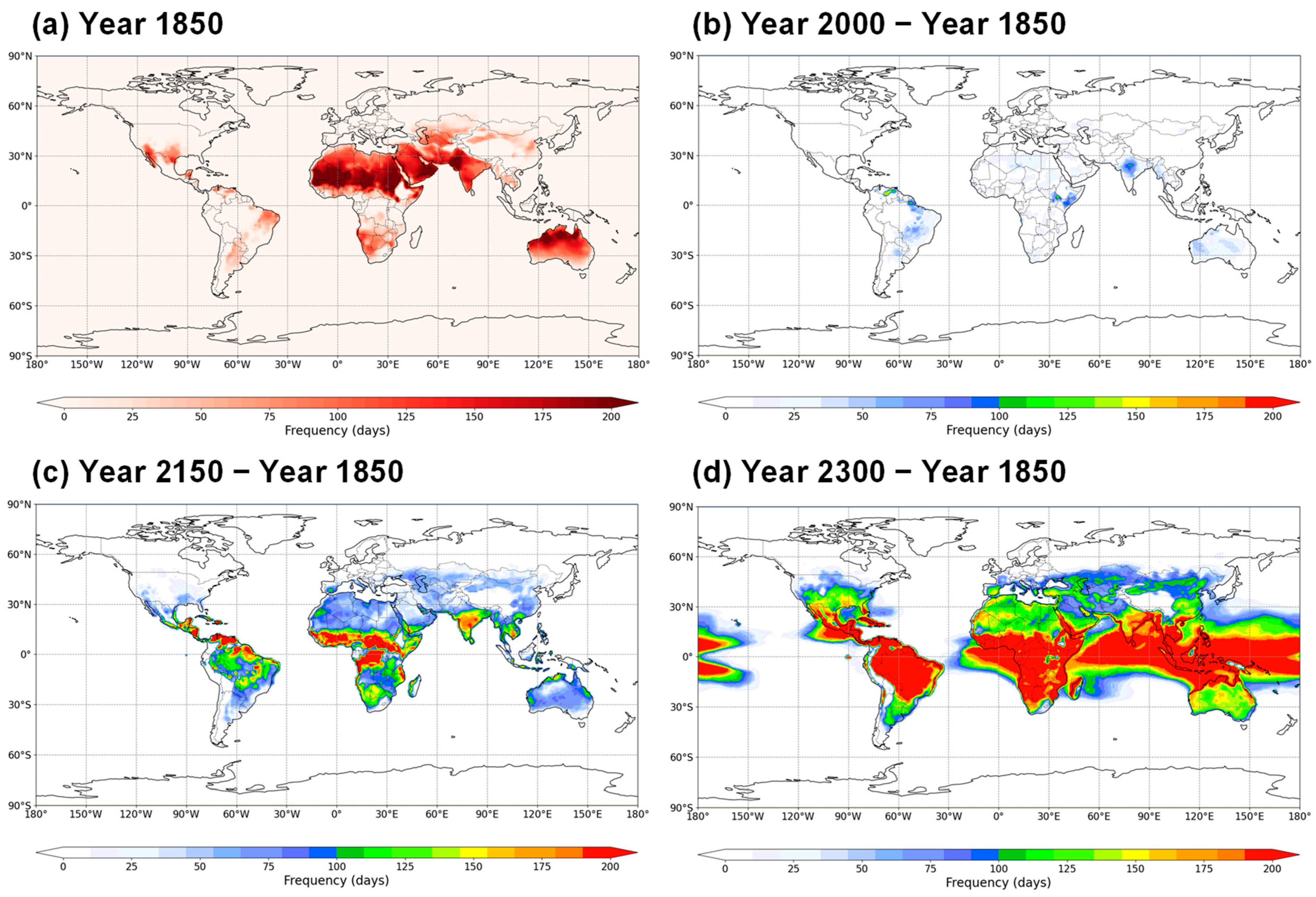
In addition to global warming trends, changes in heat wave frequency are also a critical area of research, attracting increasing attention due to their potential impacts. In Figure 3, the occurrence frequency of heat waves was defined as the total number of events where daily maximum near-surface air temperature exceeds 35 °C. In 1850, such heat wave events were primarily observed in regions such as the Sahara and Arabian Deserts, India, and Australia (Figure 3a). On a global average basis, the yearly occurrence frequency of heat waves above 35 °C in 1850 was 3.3 days, with a maximum of 221 days in the Sahara Desert. By 2000, the frequency of heat wave events above 35 °C had increased in several land regions, reflecting the early stages of global warming (Figure 3b). The unweighted global mean frequency of heat waves above 35 °C increased by 26% from 1850 to 2000. Over the 300-year period (2150−1850), the change in heat wave frequency above 35 °C, as observed in historical and SSP5-8.5 experiments, exhibited a significant increase over extensive tropical land areas (Figure 3c). The unweighted global mean frequency of heat waves above 35 °C increased by 84% from 1850 to 2150. By the year 2300, these changes are expected to become even more pronounced, with heat wave occurrence regions extending into tropical oceans and mid-latitude land areas (Figure 3d). The unweighted global mean frequency of heat waves above 35 °C increased by 317% from 1850 to 2300.

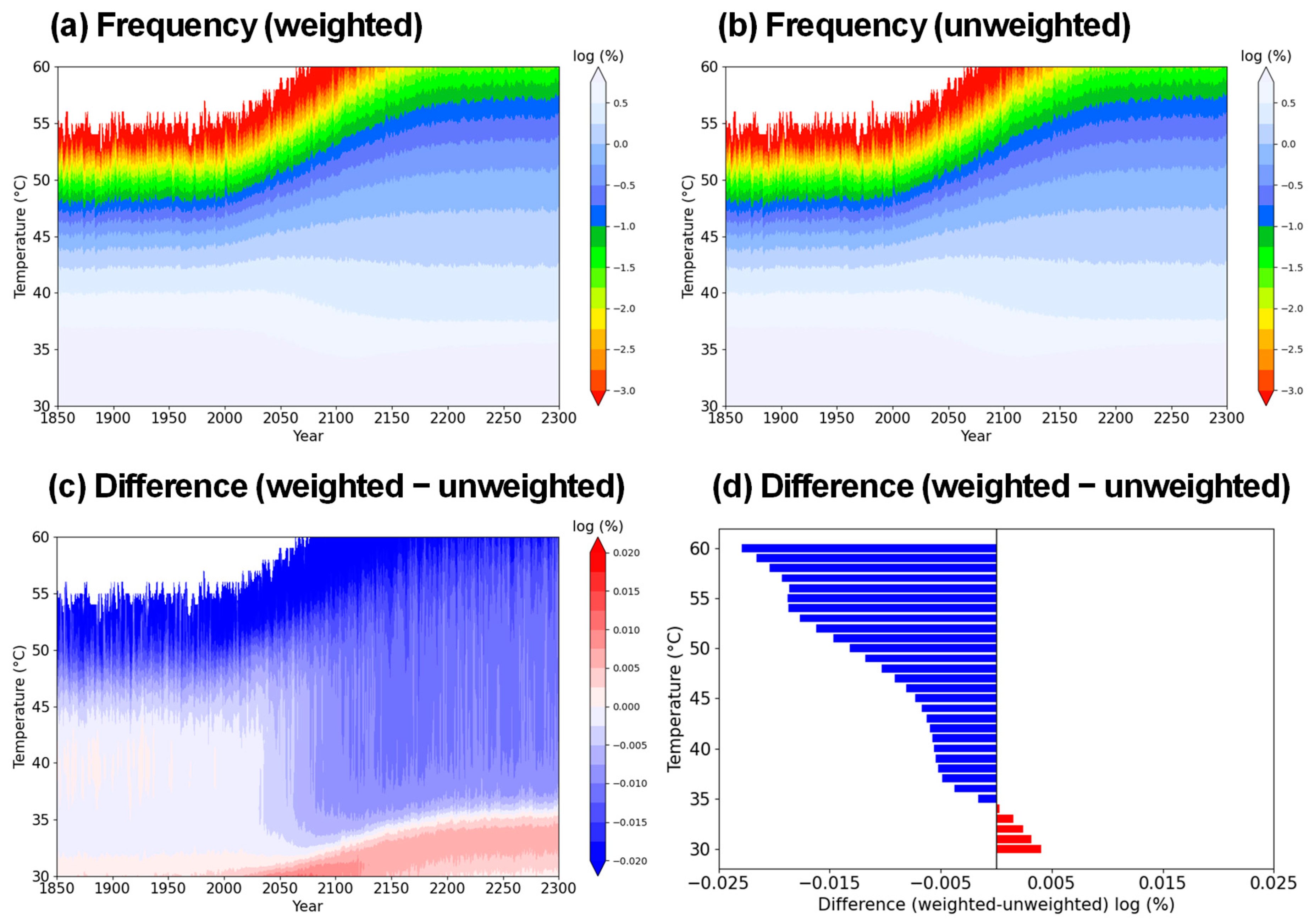
Although heat waves are relatively rare in polar regions, the heat wave frequency changes shown in Figure 3 may still be exaggerated due to the visual representation using regular latitude-longitude grids. Similar to global warming, because heat wave frequency tends to increase towards the equator, an unweighted average can yield misleading global statistics. To better understand the impact of the Earth’s curvature on global heat wave frequency, this study examined the time series of heat wave frequency for cases with and without cosine weighting for latitude (Figure 4). In Figure 4a, the x-axis represents the yearly time series from 1850 to 2300, the y-axis shows temperature thresholds in 1 °C increments, and heat wave frequency is indicated by color scales. The white areas in Figure 4a–c indicate the absence of heat wave events above the temperature thresholds specified on the y-axis. As the temperature threshold for heat waves increases, the frequency generally decreases (Figure 4a,b). Heat wave frequency increased dramatically, particularly for temperature thresholds between 45–55 °C (Figure 4a,b), consistent with global warming trends illustrated in Figure 2. For instance, although the occurrence frequency of heat waves above 54 °C in 1850 was approximately 0.0016%, it rose sharply to 0.316% by 2300, signifying a 200-fold increase over 450 years. Because the differences between the weighted and unweighted cases are difficult to distinguish visually in Figure 4a–b, the differences are depicted in Figure 4c. The weighted case displayed a lower heat wave frequency than the unweighted case in 1850 (Figure 4c). The negative difference widened by 2300 for temperature thresholds above 35 °C, whereas the frequency difference for thresholds between 30–35° became a positive value by 2300 (Figure 4c). The mean difference between the two cases over the 450-year period (1850–2300) is presented in Figure 4d. Above the 35 °C threshold, the negative difference (weighted—unweighted) in heat wave frequency was more prominent, and the difference increased with rising temperature thresholds (Figure 4d). This pattern suggests that in the weighted case, subtropical desert regions (such as the Sahara and Arabian Deserts, India, and Australia, as depicted in Figure 4a) were given less emphasis compared to the tropics near the equator. As the temperature threshold increases, the contribution of subtropical desert regions to heat wave frequency expands, which results in an increase in heat wave frequency for the weighted case at extremely high temperature thresholds (e.g., 60 °C). On the other hand, the more frequent heat waves for the 30–35 °C threshold in the weighted case can be attributed to the fact that 30–35 °C temperature events are common in tropical regions, which receive more emphasis in the weighted calculation. Therefore, if the Earth’s curvature effect is not considered, the increasing trend of heat wave frequency above 35 °C during the period 1850–2300 could be somewhat overstated, as the subtropical desert areas would be treated with the same weight as the equatorial regions. For instance, the weighted case showed an increase in heat wave frequencies compared to the unweighted case by 0.004 log (%) (base-10 logarithm of the percentage) for temperature thresholds of 30 °C, whereas the weighted case showed a reduction in heat wave frequencies compared to the unweighted case by 0.002 log (%), 0.006 log (%), 0.007 log (%), 0.013 log (%), 0.018 log (%), and 0.022 log (%) for temperature thresholds of 35 °C, 40 °C, 45 °C, 50 °C, 55 °C, and 60 °C, respectively (

Table 2. Global 450-year (1850–2300) mean heat wave frequency for the weighted case, the unweighted case, and their differences (weighted − unweighted) according to the heat wave temperature thresholds.

Temperature Threshold [°C]	30	35	40	45	50	55	60
Weighted [log (%)]	1.239	0.808	0.442	−0.007	−0.837	−2.088	−2.295
Unweighted [log (%)]	1.243	0.806	0.436	−0.014	−0.850	−2.106	−2.317
Difference [log (%)]	0.004	−0.002	−0.006	−0.007	−0.013	−0.018	−0.022

).

4. Summary and Conclusions

This study examined the effect of the Earth’s curvature on global warming and heat wave frequency changes over the period from 1850 to 2300, using data from the CMIP6 MRI-ESM2-0 historical and SSP5-8.5 experiments. By incorporating a geodetic weight that applies cosine weighting for latitude, we aimed to address the inaccuracies that arise when the curvature of the Earth is not accounted for in global climate data analysis. The spatial distributions of annual mean temperatures for 1850, 2000, 2150, and 2300 were first analyzed, revealing accelerated warming over polar regions, in addition to widespread global warming patterns in 2150 and 2300. The time series of globally averaged near-surface temperatures were then assessed for two cases: one with area weighting and one without. Due to the smaller weight applied to colder temperatures in polar regions in the weighted case, the global average temperature for 1850–2300 was found to be 8.2 °C warmer than in the unweighted case. In contrast, global warming trends for the weighted and unweighted cases were determined to be 0.276 °C per decade and 0.330 °C per decade, respectively, for the period 1850–2300. This difference likely results from a reduced temperature difference between tropical and polar regions, associated with polar amplification under global warming. Our findings suggest that if the Earth’s curvature effect is not considered, global warming trends may be overstated by about 20%.

Furthermore, this study explored changes in heat wave frequency in relation to the Earth’s curvature effect. We defined the occurrence frequency of heat waves as the total number of events with daily maximum near-surface air temperatures exceeding a given threshold. The unweighted global mean frequencies of heat waves above 35 °C were found to increase by 26% in 2000, 84% in 2150, and 317% in 2300, compared to 1850. Additionally, the weighted case consistently exhibited lower frequencies for heat waves above the 35 °C threshold than the unweighted case, due to reduced emphasis on subtropical desert regions in the weighted calculation compared to the equatorial tropics. In conclusion, the rising trend in the frequency of heat waves above 35 °C could be somewhat exaggerated (by up to 5.4% for a 60 °C threshold) if the Earth’s curvature effect is not taken into account. By addressing the potential overestimation of global warming and heat wave trends due to the neglect of the Earth’s curvature effect, this study offers valuable insights into a precise methodology for calculating global warming and heat wave trends. Future studies should continue to explore and refine these methods to ensure that climate projections are as accurate as possible, enabling better-informed policy decisions to mitigate and adapt to the effects of global climate change.