Series Solution Method Used to Solve Linear Caputo Fractional Initial Value Problems with Variable Coefficients

Abstract

Computing the solution of the linear Caputo fractional differential equation with variable coefficients cannot be obtained in closed form as in the integer-order case. However, to use ‘q’, the order of the fractional derivative, as a parameter for our mathematical model, we need to compute the solution of the equation explicitly and/or numerically. The traditional methods, such as the integrating factor or variation of parameters methods used in the integer-order case, cannot be directly applied because the product rule of the integer derivative does not hold for the Caputo fractional derivative. In this work, we present a series solution method to compute the solution of the linear Caputo fractional differential equation with variable coefficients. This provides an opportunity to compare its solution with the corresponding integer solution, namely $q=1.$ Additionally, we develop a series solution method using analytic functions in the space of $C^q$ continuous functions. We also apply this series solution method to nonlinear Caputo fractional differential equations where the nonlinearity is in the form $f(t,u)=u^2.$ We have provided numerical examples to show the application of our series solution method.

1. Introduction

Fractional differential equations have gained importance in the past four decades due to their applications in a wide range of fields such as biology, control theory, continuum mechanics, elasticity, signal analysis, quantum mechanics, bioengineering, biomedicine, mathematics, and financial systems. Many types of fractional derivatives have been introduced in the relevant literature. Among them, the Caputo derivative of order $nq,$ when $(n-1)<nq<n,$ is the closest to the integer derivative. In particular, if $q\to 1,$ then the Caputo derivative reduces to the nth order derivative. In short, the Caputo fractional differential equation of order $nq$ reduces to the nth order differential equation.

In [1], the authors demonstrated from their experiment that the mathematical model of the half-order derivative was best suited and more economical. See [1,2,3,4,5,6,7] research monographs and the references therein for the theory and applications of fractional differential equations. For some more theory, application, and computation methods of fractional differential equations, see the research articles of [1,2,3,5,7,8,9,10,11,12,13,14,15,16,17,18].

In [19], the authors demonstrated that the solution of Caputo fractional differential equations for certain values of q represents a better and more suitable mathematical model compared to the corresponding integer model. The authors achieved this by comparing their solution with the available realistic data and the solution of the corresponding integer model. The mathematical models used in [19] are simple linear Caputo fractional differential equations with constant coefficients whose solutions can be easily computed in terms of Mittag-Leffler functions. Once we compute the solution of the Caputo fractional differential equation of order $q,$ we can choose the value of q as a parameter to enhance the model.

In order to use the value of q as a parameter, we should be able to solve a variety of Caputo fractional differential equations analytically or numerically to compare it with the corresponding solution of integer order. Unfortunately, the method to solve even the linear Caputo fractional differential equations of order q ($0<q<1$), with variable coefficients, is not as routine as in the corresponding first-order differential equations. The reason is that the product rule and the variation of parameter method, which we use in solving integer-order differential equations, cannot be applied to Caputo fractional differential equations. In addition, the Mittag-Leffler function does not possess the nice properties of the exponential function as in the integer case.

So far, it has been possible to achieve methods to solve the following type of Caputo fractional differential equations:

• Caputo fractional differential equations which involve Caputo derivatives of lower order (<q) derivative terms;
• Sequential Caputo fractional differential equations with initial conditions involving Caputo fractional derivatives;
• Systems of Caputo fractional differential equations with initial conditions.

We have addressed nonhomogeneous sequential Caputo fractional differential equations with lower-order derivatives using the Laplace transform method, rather than traditional integer-order methods such as the method of undetermined coefficients or the variation of parameter methods. See [20,21,22] for the Laplace transform method for sequential Caputo fractional differential equations with fractional initial conditions and for systems of Caputo fractional differential equations with initial conditions.

In this work, we develop a series solution method to solve the following types of Caputo fractional differential equations:

• Caputo fractional differential equations of order $q,0<q<1,$ with variable coefficients;
• Nonlinear Caputo fractional differential equations.

Next, consider the linear (left sided) Caputo fractional differential equation:

$${}^{c}D_{a^{+}}^{q}u=\lambda u,a<t<b,u\left(a\right)=u_a.$$

Then, the solution of this left Caputo fractional differential equation is given by

$$u\left(t\right)=u_a{E}_{q,1}\left(\lambda {(t-a)}^q\right)=\sum _{k=0}^{\infty }{\displaystyle \frac{{\left(\lambda {(t-a)}^q\right)}^k}{\Gamma (qk+1)}}.$$

It is easy to see that this is not a $C^1$ solution, but a $C^q$ solution. See [2,4,6] for more details.

Our first main goal is to develop a method to solve a linear Caputo fractional differential equation with a variable coefficient of the following form:

$${}^{c}D_{0^{+}}^{q}u=p\left(t\right)u,u\left(a\right)=u_a.$$

(1)

The explicit solution of the linear Caputo fractional differential equation cannot be obtained in the same way as that of the integer-order case, since the Mittag-Leffler function does not have the appropriate properties of the exponential function. We assume that the solution can be expanded in the form of the $C^q$ analytic solution of the following form:

$$u\left(t\right)=u_0+u_1{\displaystyle \frac{{(t-a)}^q}{\Gamma (q+1)}}+u_2{\displaystyle \frac{{(t-a)}^{2q}}{\Gamma (2q+1)}}+\dots +u_n{\displaystyle \frac{{(t-a)}^{nq}}{\Gamma (nq+1)}}+\dots .$$

(2)

In addition, we assume that the variable coefficient $p\left(t\right)$ can also be expanded in the following $C^q$ analytic form:

$$p\left(t\right)=p_0+p_1{\displaystyle \frac{{(t-a)}^q}{\Gamma (q+1)}}+p_2{\displaystyle \frac{{(t-a)}^{2q}}{\Gamma (2q+1)}}+\dots +p_n{\displaystyle \frac{{(t-a)}^{nq}}{\Gamma (nq+1)}}+\dots .$$

(3)

Using these relations (2) and (3), we have obtained the series solution representation form for the solution of (1). We have applied it to several examples of $p\left(t\right)$ and presented some numerical results. In all of these examples, we have achieved the integer order result as a special case, that is, when $q=1$.

Using the same technique as in our next main result, we have obtained the series solution form for the nonlinear Caputo fractional differential equation:

$${}^{c}D_{0^{+}}^{q}u=u^2,u\left(0\right)=u_0.$$

Note that when $q=1,$ computing the solution is very trivial using the separation of variables method. However, solving the above nonlinear differential equation is applicable in blow-up problems. The solution plays an important role in finding the blow-up time for time fractional reaction–diffusion equations. See [23] for more details. We have presented numerical examples for the nonlinear problem of different values of q, including $q=1$ in our main results.

The organization of our research article is as follows: In Section 2, we recall relevant definitions and known results related to our main results. In Section 3, we present two main results. In the first main result, we obtain the solution formula for linear Caputo fractional differential equations with variable coefficients. In our second main result, we derive the series solution formula for a specific nonlinear Caputo fractional differential equation. We also present several numerical examples as applications of our main results.

2. Preliminary Results

In this section, we introduce important fractional calculus topics, setting the stage for our discussion. We provide several basic definitions of fractional derivatives and integrals, explain their properties, and highlight key mathematical results.

Definition 1.

The Gamma function of order q is defined by

$$\Gamma \left(q\right)={\int }_0^{\infty }{t}^{q-1}{e}^{-t}dt,$$

where $0<q\le 1$.

Definition 2.

The Riemann–Liouville fractional integral of $u\left(t\right)$ of order q is defined by

$$D_{0+}^{-q}u\left(t\right)={\displaystyle \frac{1}{\Gamma \left(q\right)}}{\int }_0^t{(t-s)}^{q-1}u\left(s\right)ds,t>0,$$

where $0<q\le 1$ and $\Gamma \left(q\right)$ is the Gamma function.

The Caputo integral of order q for any function is the same as that of the Riemann–Liouville integral of order $q.$

Definition 3.

The Riemann–Liouville (left-sided) fractional derivative of $u\left(t\right)$ of order q, when $0<q\le 1$, is defined as follows:

$$D_{0+}^{q}u\left(t\right)={\displaystyle \frac{1}{\Gamma (1-q)}}{\displaystyle \frac{d}{dt}}{\int }_0^t{(t-s)}^{q-1}u\left(s\right)ds,t>0.$$

Definition 4.

The Caputo (left-sided) fractional derivative of $u\left(t\right)$ of order $nq$, when $n-1<nq<n$, is given by

$${}^{c}D_{a^{+}}^{nq}u\left(t\right)={\displaystyle \frac{1}{\Gamma (n-nq)}}{\int }_a^t{(t-s)}^{n-nq-1}{u}^{\left(n\right)}\left(s\right)ds,t>a,$$

and the (right-sided) fractional derivative is given by

$${}^{c}D_{b^{-}}^{nq}u\left(t\right)={\displaystyle \frac{{(-1)}^n}{\Gamma (n-nq)}}{\int }_t^b{(s-t)}^{n-nq-1}{u}^{\left(n\right)}\left(s\right)ds,t<b,$$

where $u^{\left(n\right)}\left(t\right)={\displaystyle \frac{d^n\left(u\right)}{d{t}^n}}$.

In particular, if q is an integer, then the Caputo derivative and the integer derivative are one and the same.

See [3,4,6] for more details on the Caputo and Riemann–Liouville fractional derivative.

Definition 5.

The Caputo (left) fractional derivative of $u\left(t\right)$ of order q, when $0<q<1$, is defined as follows:

$${}^{c}D_{0+}^{q}u\left(t\right)={\displaystyle \frac{1}{\Gamma (1-q)}}{\int }_0^t{(t-s)}^{-q}{u}^{\prime }\left(s\right)\mathrm{d}s.$$

We are simply replacing n with 1 in the above definition of the Caputo derivative of order $nq$.

The following definition is useful in Caputo fractional differential equations.

Definition 6.

If the Caputo derivative of a function $u\left(t\right)$ of order q, $0<q\le 1,$ exists on an interval $J=[0,T],T>0,$ then we say, $u\in C^q(J,R).$

Note that all $C^1$ functions on $[0,t]$ are $C^q$ functions on $[0,t]$. However, the converse need not be true.

Next, we define the Mittag-Leffler function, which will be useful in solving systems of linear Caputo fractional differential equations. See [7] for more on fractional differential equations with applications.

Definition 7.

The two parameter Mittag-Leffler function is defined as

$$E_{q,r}\left(\lambda t^q\right)=\sum _{k=0}^{\infty }{\displaystyle \frac{{\left(\lambda t^q\right)}^k}{\Gamma (qk+r)}},$$

(4)

where q, $r>0$, and λ is a constant.

It is a generalization of the exponential function and plays the same role for fractional differential equations as the exponential function does for integer derivative dynamic equations, especially when $0<q<1$.

Furthermore, for $r=q$ and $r=1$, it will be denoted by $E_{q,q}\left(\lambda t^q\right)$ and $E_{q,1}\left(\lambda t^q\right)$, respectively. This form of the Mittag-Leffler function is useful to solve the qth order linear Caputo fractional differential equation.

If $q=1$ and $r=1$ in (4), then we have the following:

$$E_{1,1}\left(\lambda t\right)=\sum _{k=0}^{\infty }{\displaystyle \frac{{\left(\lambda t\right)}^k}{\Gamma (k+1)}}=e^{\lambda t},$$

where $e^{\lambda t}$ is the usual exponential function. In addition, Mittag-Leffler functions with $r=1$ and $r=q$ with $0<q<1$, will be useful when sequential derivatives are involved in the fractional differential equation.

See [3,4,6] for more details on the Mittag-Leffler functions.

Since we are finding the solutions to Caputo fractional differential equations that yield the integer order derivative result as a special case, we need the sequential Caputo fractional derivative of order $nq$.

Definition 8.

The Caputo fractional derivative of $u\left(t\right)$ of order $nq$ for $n-1<nq<n$ is said to be sequential Caputo fractional derivative of order q, if the relation

$${}^{c}D_{0+}^{nq}u\left(t\right)={}^{c}D_{0+}^q{(}^c{D}_{0+}^{(n-1)q})u\left(t\right),$$

(5)

holds for $n=2,3\dots$.

Note that the Equation (5) can also be written as

$${}^{c}D_{0+}^{kq}u\left(t\right)={}^{c}D_{0+}^q{(}^c{D}_{0+}^q){(}^c{D}_{0+}^q)\dots ktimes\dots {(}^c{D}_{0+}^q)u\left(t\right),$$

for $k=2,3,4\dots$.

In general, the Caputo fractional derivative is not sequential, whereas the integer derivative is always sequential. To find the general solution of the homogeneous sequential Caputo fractional differential equation using $E_{q,1}\left(\lambda t^q\right)$, we also require the initial conditions to be in the terms of the Caputo fractional derivative of the following form:

$${(}^c{D}_{0+}^{kq})u\left(t\right){|}_{t=0}=b_k,(b_k\in R;k=0,1,\dots ,n-1).$$

See [20,21,24] for some more work on sequential fractional differential equations.

Next, we consider the Caputo fractional homogeneous linear fractional differential equation of order q, where $0<q<1$ alongside the initial conditions take the following form:

$${}^{c}D_{0^{+}}^{q}u\left(t\right)-\lambda u\left(t\right)=0,t>0,u\left(0\right)=u_0.$$

(6)

Then, the solution of (6) can be obtained as follows:

$$u\left(t\right)=u_0{E}_{q,1}\left(\lambda t^q\right),$$

where $\lambda$ is a constant.

Note that the solution of the (6) is only a $C^q$ solution. It will be a $C^1$ solution only when $q=1.$

Remark 1.

The solution of (6) cannot be obtained if λ is replaced by a function of t using the method of integrating factor as in the integer order case. We cannot even solve (6) using the Laplace transform method.

Now, consider the equation

$${}^{c}D_{0^{+}}^{nq}u\left(t\right)-\lambda u\left(t\right)=0,u^k\left(0\right)=b_k,k=0,1,2,3,\dots ,n-1,$$

(7)

where $n-1<nq<n.$ See [4,6] for the details of the solution when $\lambda$ is a constant.

Remark 2.

The Equation (7) cannot be solved if the Caputo fractional differential equation has lower-order terms of ${}^{c}D_{0^{+}}^{kq}u\left(t\right)$ for any integer $k,$$k=0,1,2,3,\dots ,(n-1),$

(a) with constant coefficients;

(b) with variable coefficients.

In order to address part (a) of Remark 2, we assumed that the Caputo fractional differential operator ${}^{c}D^{nq}$ is sequential. See [20,21] for more details on the sequential fractional differential equation.

In this work, we addressed part (b) for (6) when $\lambda$ is a function of t.

3. Main Results

In this section, we establish a series solution method to solve linear Caputo fractional differential equations of order q, where $0<q<1$ with variable coefficients. We seek a solution in the space of $C^q$ continuous functions instead of the $C^1$ function as in the literature. We used the method to solve nonlinear Caputo fractional differential equations, when the nonlinear term is $f\left(u\right)=u^2$.

Consider the linear Caputo fractional differential equation with variable coefficient of the form

$${}^{c}D_{0^{+}}^{q}u=p\left(t\right)u,u\left(0\right)=u_0.$$

(8)

We assume that the solution of the Caputo fractional differential Equation (8) has Taylor series expansion in powers of $t^q.$ That is, we can write the solution as

$$\begin{array}{cc}\hfill u\left(t\right)& =u_0+u_1{\displaystyle \frac{t^q}{\Gamma (q+1)}}+u_2{\displaystyle \frac{t^{2q}}{\Gamma (2q+1)}}+\dots +u_n{\displaystyle \frac{t^{nq}}{\Gamma (nq+1)}}+\dots ,\hfill \\ \hfill & =\sum _{k=0}^{\infty }{u}_k{\displaystyle \frac{t^{kq}}{\Gamma (kq+1)}}.\hfill \end{array}$$

(9)

Similarly, we assume that the coefficient $p\left(t\right),$ in the Equation (8) can be expanded as

$$\begin{array}{cc}\hfill p\left(t\right)& =p_0+p_1{\displaystyle \frac{t^q}{\Gamma (q+1)}}+p_2{\displaystyle \frac{t^{2q}}{\Gamma (2q+1)}}+\dots +p_n{\displaystyle \frac{t^{nq}}{\Gamma (nq+1)}}+\dots ,\hfill \\ \hfill & =\sum _{k=0}^{\infty }{p}_k{\displaystyle \frac{t^{kq}}{\Gamma (kq+1)}}.\hfill \end{array}$$

(10)

Lemma 1.

Let the functions $u\left(t\right)$ and $p\left(t\right)$ have the series expansion of the form (9) and (10). Then the product function can be expressed as a series function of the form

$$\begin{array}{cc}\hfill p\left(t\right)u\left(t\right)& =U_0+U_1{t}^q+U_2{t}^{2q}+\dots +U_{2n-1}{t}^{(2n-1)q}+U_{2n}{t}^{2nq}+\dots ,\hfill \\ \hfill & =\sum _{k=0}^{\infty }{U}_k{t}^{kq}.\hfill \end{array}$$

(11)

Here, the even $U_{2n}$ and the odd $U_{2n-1}$ terms are given by

$$U_{2n}=\sum _{i=0}^{2n}{\displaystyle \frac{p_{(2n-i)}{u}_i}{\Gamma \left(\right(2n-i)q+1)\Gamma (iq+1)}},\mathrm{for}n=0,1,2,\dots ,$$

(12)

$$U_{2n-1}=\sum _{i=0}^{2n-1}{\displaystyle \frac{p_{(2n-1-i)}{u}_i}{\Gamma \left(\right(2n-1-i)q+1)\Gamma (iq+1)}},\mathrm{for}n=1,2,\dots ,$$

(13)

Proof. 

It is easy to see that that

$$U_0=p_0{u}_0,$$

and

$$U_1={\displaystyle \frac{p_1{u}_0+p_0{u}_1}{\Gamma (q+1)}},$$

by directly looking at the constant term and the coefficient of $t^q$ in the product function $p\left(t\right)u\left(t\right).$ This clearly verifies the Formulas (12) and (13) for $n=0$ and $n=1,$ respectively.

Similarly, observing the coefficient of $t^{2q}$ and $t^{3q}$, respectively, in the product function $p\left(t\right)u\left(t\right)$, we obtain

$$\begin{array}{cc}\hfill U_2& ={\displaystyle \frac{p_0{u}_2}{\Gamma (2q+1)}}+{\displaystyle \frac{p_1{u}_1}{\Gamma (q+1)\Gamma (q+1)}}+{\displaystyle \frac{p_2{u}_0}{\Gamma (2q+1)}},\hfill \end{array}$$

and

$$\begin{array}{cc}\hfill U_3& ={\displaystyle \frac{p_0{u}_3}{\Gamma (3q+1)}}+{\displaystyle \frac{p_2{u}_1}{\Gamma (2q+1)\Gamma (q+1)}}+{\displaystyle \frac{p_1{u}_2}{\Gamma (q+1)\Gamma (2q+1)}}+{\displaystyle \frac{p_3{u}_0}{\Gamma (3q+1)}},\hfill \end{array}$$

respectively. This verifies the Formulas (12) and (13) for $n=1$ and $n=2,$ respectively. Generalizing this for the coefficient of $t^{2nq}$ and $t^{(2n-1)q}$, it is easy to check whether Formulas (12) and (13) hold true for $n\ge 0$ and $n\ge 1,$ respectively. □

Theorem 1.

Let the functions $u\left(t\right)$ and $p\left(t\right)$ have the series expansion of the form (9) and (10). Then, the solution $u\left(t\right)$ is given by

$$u\left(t\right)=u_0+\sum _{k=1}^{\infty }{\displaystyle \frac{u_{2k-1}}{\Gamma \left(\right(2k-1)q+1)}}{t}^{(2k-1)q}+\sum _{k=1}^{\infty }{\displaystyle \frac{u_{2k}}{\Gamma (2kq+1)}}{t}^{\left(2k\right)q},$$

(14)

where

$$u_{2n+1}=\Gamma (2nq+1)\sum _{i=0}^{2n}{\displaystyle \frac{p_{(2n-i)}{u}_i}{\Gamma \left(\right(2n-i)q+1)\Gamma (iq+1)}},\mathrm{for}n=0,1,2,\dots$$

(15)

and

$$u_{2n}=\Gamma ((2n-1)q+1)\sum _{i=0}^{2n-1}{\displaystyle \frac{p_{(2n-1-i)}{u}_i}{\Gamma \left(\right(2n-1-i)q+1)\Gamma (iq+1)}},\mathrm{for}n=1,2,\dots$$

(16)

Proof. 

From Equation (9), we obtain

$$\begin{array}{cc}\hfill {}^{c}D_{0^{+}}^{q}u& =u_1+u_2{\displaystyle \frac{t^q}{\Gamma (q+1)}}+\dots +u_{n+1}{\displaystyle \frac{t^{nq}}{\Gamma (nq+1)}}+\dots \hfill \\ \hfill & =\sum _{k=1}^{\infty }{u}_k{\displaystyle \frac{t^{(k-1)q}}{\Gamma \left(\right(k-1)q+1)}}.\hfill \end{array}$$

(17)

Now, using (8), (11), and (17), we obtain

$$\sum _{k=1}^{\infty }{u}_k{\displaystyle \frac{t^{(k-1)q}}{\Gamma \left(\right(k-1)q+1)}}=\sum _{k=0}^{\infty }{U}_k{t}^{kq}.$$

(18)

But

$$\sum _{k=0}^{\infty }{U}_k{t}^{kq}=\sum _{k=1}^{\infty }{U}_{(k-1)}{t}^{(k-1)q},$$

From the relation (18), equating the coefficient of $t^{lq}$, we obtain

$$u_l=(\Gamma (l-1)q+1)U_{l-1}.$$

(19)

This implies

$$u_1=\Gamma \left(1\right)U_0=p_0{u}_0,$$

and

$$u_2=\Gamma (q+1)U_1=p_1{u}_0+p_0{u}_1=(p_0^2+p_1)u_0.$$

In general, for $l=2n$ and $l=2n+1$ on (19), we will have the relation

$$u_{2n}=\Gamma ((2n-1)q+1)U_{2n-1},$$

and

$$u_{2n+1}=\Gamma (2nq+1)U_{2n}.$$

This concludes the proof by using Lemma 1 and substituting the value of $U_{2n-1}$ and $U_{2n}$ to compute $u_{2n}$ and $u_{2n+1},$ for $n=1,2,\dots$. □

Remark 3.

It is easy to observe that, in the solution of (8), we can compute the $u_{2n}\left(t\right)$ and $u_{2n+1}\left(t\right)$ by induction since the computation of $u_{n+1}$ depends on all the terms of $u_i$ for $i=1,2,\dots n.$ Here, we compute a couple of terms $u_i$ for $i=1,2,3$ and 4 using the results of Theorem 1.

$$\begin{array}{cc}\hfill u_1& =u_0{p}_0,\hfill \\ \hfill u_2& =u_0(p_0^2+p_1),\hfill \\ \hfill u_3& =u_0\left[p_0^3+p_0{p}_1\{1+{\displaystyle \frac{\Gamma (2q+1)}{{(\Gamma (q+1))}^2}}\}+p_2\right],\hfill \\ \hfill u_4& =u_0\left[p_0^4+p_0^2{p}_1\{1+{\displaystyle \frac{\Gamma (2q+1)}{{(\Gamma (q+1))}^2}}+{\displaystyle \frac{\Gamma (3q+1)}{\Gamma (2q+1)\Gamma (q+1)}}\}\right],\hfill \\ \hfill & +u_0\left[p_0{p}_2\{1+{\displaystyle \frac{\Gamma (3q+1)}{\Gamma (2q+1)\Gamma (q+1)}}\}+p_1^2{\displaystyle \frac{\Gamma (3q+1)}{\Gamma (2q+1)\Gamma (q+1)}}+p_3\right].\hfill \end{array}$$

This can be generalized for any $n.$ We leave it as an exercise.

We have already obtained the series solution of the Caputo fractional initial value problem (8) when $p\left(t\right)$ is constant. See [22] for more details for the solution. Additionally, see [20,25] for a numerical and symbolic method of finding the solution of the Caputo fractional differential equation with variable coefficients.

4. Numerical Results

In this section, we have provided several examples as applications of our main results.

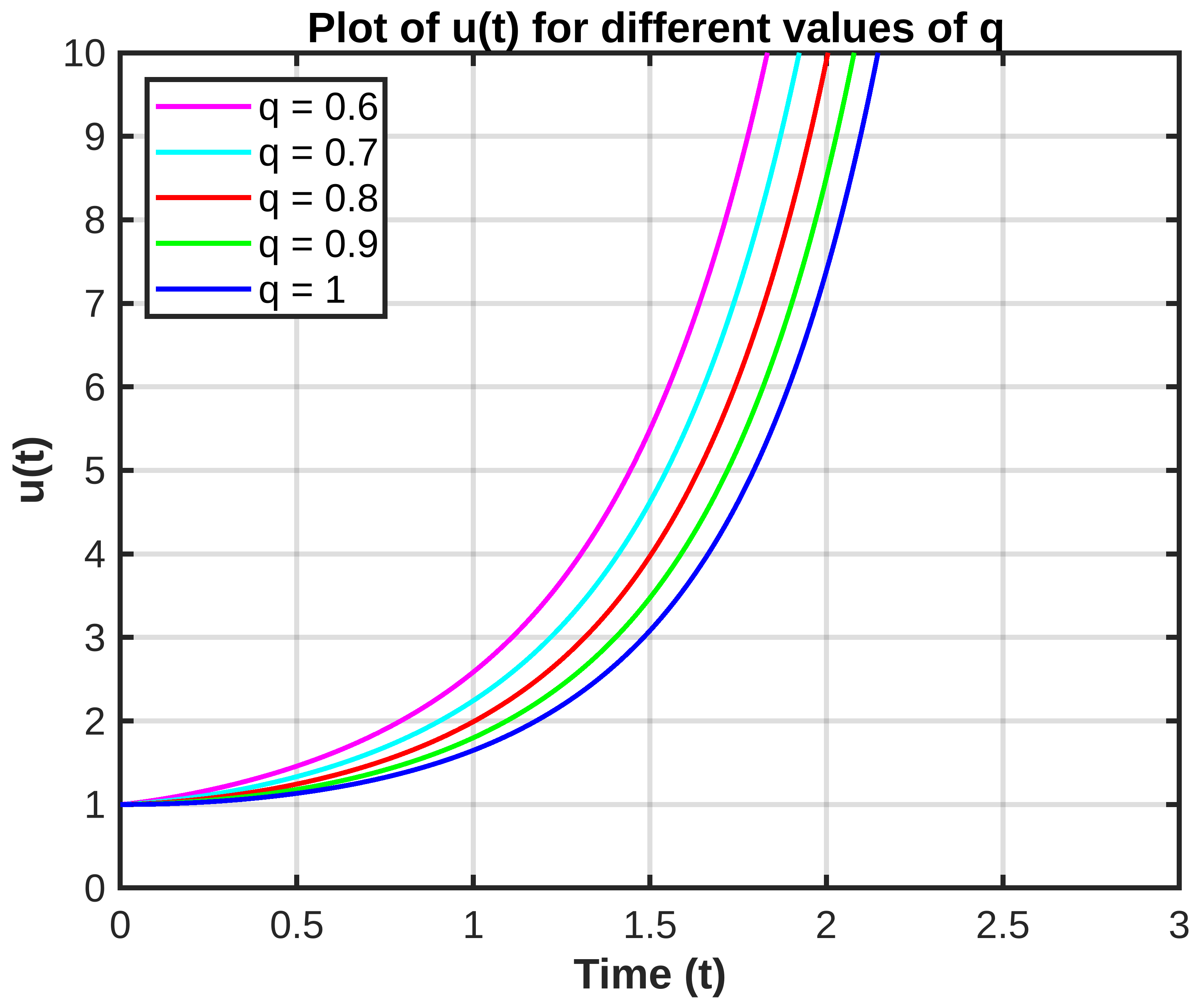
Example 1.

Consider (8) when $p\left(t\right)=t^q.$ In this case, $p_0=0,p_1=\Gamma (q+1),$ and $p_i\equiv 0,\mathrm{for}i=2,3,\dots$; using the relation (14), (15), and (16), the solution is given by

$$u\left(t\right)=u_0\left[1+\sum _{n=1}^{\infty }\prod _{k=1}^n{\displaystyle \frac{\Gamma ((2k-1)q+1)t^{2nq}}{\Gamma (2kq+1)}}\right].$$

Here, in Figure 1, we have drawn the graph of the solution $u\left(t\right),$ when $p\left(t\right)=t^q$ for different values of q, specifically $q=0.6, 0.7, 0.8, 0.9,$ and $1.$ We used MATLAB to plot the graph.

Example 2.

Consider (8) when $p\left(t\right)=t^{2q}.$ In this case, $p_0=0,p_1=0,p_2=\Gamma (2q+1)$, $p_i\equiv 0,\mathrm{for}i=3,4,\dots$; using the relation (14), (15), and (16), the solution is given by

$$u\left(t\right)=u_0\left[1+\sum _{n=1}^{\infty }\prod _{k=1}^n{\displaystyle \frac{\Gamma ((3k-1)q+1)t^{3nq}}{\Gamma (3kq+1)}}\right].$$

In Figure 2, we have drawn the graph of the solution $u\left(t\right),$ when $p\left(t\right)=t^{2q}$ for different values of q, specifically $q=0.6, 0.7, 0.8, 0.9,$ and $1.$ For $q=1$, we obtained the integer result which is well known. However, our solution might match with the realistic data for some $q<1$. Based on the realistic data, we can choose the value of q which more closely fits the data. In short, the value of q can be used as a parameter to enhance the mathematical model. This has been achieved in [19] using linear Caputo fractional differential equations with constant coefficients whose solutions are in terms of Mittag-Leffler functions.

The application of our result of the series solution method developed for the linear Caputo fractional differential Equation (8) can now be used to solve the nonlinear Caputo fractional differential equation.

Example 3.

Consider the nonlinear Caputo fractional differential equation

$${}^{c}D_{0^{+}}^{q}u=u^2,u\left(0\right)=u_0.$$

(20)

It is easy to see that when $q=1,$ one can solve the first order differential equation

$$u^{\prime }=u^2,u\left(0\right)=u_0,$$

explicitly using the separation of variables. In particular, if $u_0=1,$ the solution is given by $u\left(t\right)={\displaystyle \frac{1}{1-t}}.$ This solution blows up at $t=1.$ Although one cannot find the solution of (20) for any $q<1$ in explicit form, the blow-up time can be estimated using the explicit solution of (20) for $q=1.$ See [23] for more details.

Now applying Theorem 1, with $p\left(t\right)=u\left(t\right)$, we obtain,

$$u_{2n+1}=\Gamma (2nq+1)\sum _{i=0}^{2n}{\displaystyle \frac{u_{(2n-i)}{u}_i}{\Gamma \left(\right(2n-i)q+1)\Gamma (iq+1)}},\mathrm{for}n=0,1,2,\dots$$

(21)

and

$$u_{2n}=\Gamma ((2n-1)q+1)\sum _{i=0}^{2n-1}{\displaystyle \frac{u_{(2n-1-i)}{u}_i}{\Gamma \left(\right(2n-1-i)q+1)\Gamma (iq+1)}},\mathrm{for}n=1,2,\dots$$

(22)

Using the Equation (21) and (22), we obtain

$$\begin{array}{cc}\hfill u_1& =u_0^2,\hfill \\ \hfill u_2& =\Gamma (q+1){\displaystyle \frac{2u_1{u}_0}{\Gamma (q+1)}}=2u_0^3,\hfill \\ \hfill u_3& =\Gamma (2q+1)\left[{\displaystyle \frac{2u_2{u}_0}{\Gamma (2q+1)}}+{\displaystyle \frac{u_1^2}{{(\Gamma (q+1))}^2}}\right].\hfill \end{array}$$

Substituting $u_1 \mathrm{and}$$u_2$ in the formula for $u_3$ above, then we obtain,

$$\begin{array}{cc}\hfill u_3& =u_0^4\left[2^2+{\displaystyle \frac{\Gamma (2q+1)}{{(\Gamma (q+1))}^2}}\right],\hfill \\ \hfill u_4& =u_0^5\left[2^3+{\displaystyle \frac{2\Gamma (2q+1)}{{(\Gamma (q+1))}^2}}+{\displaystyle \frac{2^2\Gamma (3q+1)}{\Gamma (q+1)\Gamma (2q+1)}}\right].\hfill \end{array}$$

Now, using the Formula (21), we obtain

$$\begin{array}{cc}\hfill u_5& =u_0^6[2^4+{\displaystyle \frac{2^2\Gamma (2q+1)}{{(\Gamma (q+1))}^2}}+{\displaystyle \frac{2^3\Gamma (3q+1)}{\Gamma (q+1)\Gamma (2q+1)}}+{\displaystyle \frac{2^3\Gamma (4q+1)}{\Gamma (q+1)\Gamma (3q+1)}}\hfill \\ \hfill & +{\displaystyle \frac{2\Gamma (2q+1)\Gamma (4q+1)}{\Gamma (3q+1){(\Gamma (q+1))}^3}}+{\displaystyle \frac{2^2\Gamma (4q+1)}{{(\Gamma (2q+1))}^2}}].\hfill \end{array}$$

In particular, if $u_0=1,$ then

$$\begin{array}{cc}\hfill u_1& =1,\hfill \\ \hfill u_2& =2,\hfill \\ \hfill u_3& =2^2+{\displaystyle \frac{\Gamma (2q+1)}{{(\Gamma (q+1))}^2}},\hfill \\ \hfill u_4& =2^3+{\displaystyle \frac{2\Gamma (2q+1)}{{(\Gamma (q+1))}^2}}+{\displaystyle \frac{2^2\Gamma (3q+1)}{\Gamma (q+1)\Gamma (2q+1)}},\hfill \\ \hfill u_5& =2^4+{\displaystyle \frac{2^2\Gamma (2q+1)}{{(\Gamma (q+1))}^2}}+{\displaystyle \frac{2^3\Gamma (3q+1)}{\Gamma (q+1)\Gamma (2q+1)}}+{\displaystyle \frac{2^3\Gamma (4q+1)}{\Gamma (q+1)\Gamma (3q+1)}}\hfill \\ \hfill & +{\displaystyle \frac{2\Gamma (2q+1)\Gamma (4q+1)}{\Gamma (3q+1){(\Gamma (q+1))}^3}}+{\displaystyle \frac{2^2\Gamma (4q+1)}{{(\Gamma (2q+1))}^2}}.\hfill \end{array}$$

Now an approximate solution of (20) when $u_0=1$ is given by

$$u\left(t\right)\approx 1+u_1{\displaystyle \frac{t^q}{\Gamma (q+1)}}+u_2{\displaystyle \frac{t^{2q}}{\Gamma (2q+1)}}+u_3{\displaystyle \frac{t^{3q}}{\Gamma (3q+1)}}+u_4{\displaystyle \frac{t^{4q}}{\Gamma (4q+1)}})+u_5{\displaystyle \frac{t^{5q}}{\Gamma (5q+1)}}.$$

(23)

In particular, (23) simplifies to

$$u\left(t\right)\approx 1+t+t^2+t^3+t^4+t^5,$$

for $q=1.$ This is basically Taylor’s approximation of the first six terms of the solution of

$$u^{\prime }=u^2,u\left(0\right)=1,$$

which is $u={\displaystyle \frac{1}{1-t}}.$

In Figure 3, we have drawn the graphs of the solution of (20), using the first six terms of the sequence for $q=0.6, 0.7, 0.8, 0.9$, and 1. It is easy to see that the graph for $q=0.6$ is above the graph of $q=0.7$ and so on. It is easy to see that the solution is a decreasing function of $q.$

We know that the solution for $q=1$ can easily be computed as $u={\displaystyle \frac{1}{1-t}},$ which blows up at $t=1$. From our graphical approach, we can show that the solution graph for $q=0.9$ blows up before $t=1$. Similarly, the other graphs for $q<0.9$ blow up before the solution graph of $q=0.9$. Theoretically, the earlier blow-up time for $q<1$ has been established in [23]. By computing a few more terms, we can compute the blow-up time with a better approximation.

5. Conclusions

In our earlier work, we solved sequential Caputo fractional differential equations with fractional initial conditions using the Laplace transform method and the series solution method. In this research article, we have developed a series solution method to solve the solution of Caputo fractional differential equations of order $q, 0<q<1,$ with variable coefficients in the space of $C^q$ continuous functions. We have also applied the series solution method to solve nonlinear Caputo fractional differential equations, which is useful in blow-up problems. It remains an open problem whether we can develop MATLAB or Python code to solve a linear Caputo fractional differential equation with variable coefficients and initial conditions, as in the integer case. This is essential for solving nonlinear Caputo fractional differential equations with variable coefficients using the generalized quasilinearization method. It is also still an open question whether we can solve sequential Caputo fractional differential equations using the series solution method. In our future work, we plan to consider a sequential $2q$ order Caputo fractional differential equation with variable coefficients, such as

$${}^{c}D_{0^{+}}^{2q}u+p{\left(t\right)}^c{D}_{0^{+}}^{q}u+q\left(t\right)u=0,u\left(0\right)=u_0,{}^{c}D_{0^{+}}^q{u\left(t\right)|}_{t=0}=u_1.$$

The analytical solution of the above equation, even for $q=1$, is not available in the current literature.