Modeling and Visualizing the Dynamic Spread of Epidemic Diseases—The COVID-19 Case

Abstract

Our aim is to provide an insight into the procedures and the dynamics that lead the spread of contagious diseases through populations. Our simulation tool can increase our understanding of the spatial parameters that affect the diffusion of a virus. SIR models are based on the hypothesis that populations are “well mixed”. Our model constitutes an attempt to focus on the effects of the specific distribution of the initially infected individuals through the population and provide insights, considering the stochasticity of the transmission process. For this purpose, we represent the population using a square lattice of nodes. Each node represents an individual that may or may not carry the virus. Nodes that carry the virus can only transfer it to susceptible neighboring nodes. This important revision of the common SIR model provides a very realistic property: the same number of initially infected individuals can lead to multiple paths, depending on their initial distribution in the lattice. This property creates better predictions and probable scenarios to construct a probability function and appropriate confidence intervals. Finally, this structure permits realistic visualizations of the results to understand the procedure of contagion and spread of a disease and the effects of any measures applied, especially mobility restrictions, among countries and regions.

1. Introduction

This research aims to provide a supplementary tool, improving our ability to understand, trace and visualize the epidemic and pandemic spread of viruses in populations, considering specific spatial information. Our main purpose is to provide an appropriate model to understand the diffusion mechanisms and the effects of different population characteristics and restrictive measures as accurately as possible.

As a reference, we used parameters that are estimated as applicable on COVID-19 in Greece. It is an appropriate example, since it constitutes a coronavirus disease (COVID), first observed during the last days of 2019. An individual can become infected by close contact, being in indoor settings or even by touching contaminated surfaces or objects. Carriers can be symptomatic or asymptomatic. Both categories of carriers can become contagious. One year later, the first vaccine was available, and now, nine vaccines have been approved [1].

The most common model to approach the spread of a virus disease is using SIR [2]. A homogenous population of size N is divided into three groups: susceptible (S), infected (I) and removed (R). Susceptible individuals can become infected by contagious infected individuals, while infected individuals can become removed, either by being recovered (and immune) or dead. Obviously, at any given time t:

$$N\left(t\right)=S\left(t\right)+I\left(t\right)+R\left(t\right).$$

(1)

Continuous time epidemic models, such as SIR, are usually applied to describe the dynamics of transmission of infectious diseases, because of their tractability [3,4,5]. Parameters are easier to predict, and the results provide interesting insights.

Additional conditions are allowed in more recent models. In the case of another coronavirus syndrome, which broke out in South Korea, the model additionally included people who were exposed to the virus (E), asymptomatic carriers (A) and hospitalized heavily diseased individuals (H) [6].

The model works as follows: susceptible individuals might become exposed, if they are in contact with infected or asymptomatic individuals. After an incubation period, exposed individuals become infectious–contagious. Some of them are symptomatic (Infected), while others are asymptomatic. Some of the symptomatic individuals are hospitalized, and all asymptomatic, infected and hospitalized individuals move to removed (recover or die).

Recent research on COVID-19 additionally separated recovered from symptomatic individuals (R), those who are observable and have recovered from being asymptomatic (AR), and those who cannot be identified easily. They also added a spatial parameter: the density of the population [7]. This consideration of heterogeneous populations and their effect on the spread of the virus was an inspiration for our research.

Additionally, innovative research on COVID-19 introduced the possibility of contagion through viral shedding in the environment, including a pathogen (P) variable too [8].

On the other hand, there are researchers that use a simulation procedure, considering that the density of individuals infected by COVID-19 in a population could be fitted well by a self-organizing diffusion model (SODM), designed to describe the diffusion of a charge through a lattice. Considering a square lattice of nodes that can be active or inactive (representing carriers or non-carriers), they assign a “charge” instead of the virus on some nodes that become active (carriers). Charge can be transferred to inactive nodes neighboring to an active node [9].

Difference equations are also appropriate, since they could be directly applicable to time series data [5]; we choose to work using a simulation, which might be more accurate and adapted to the time series data available if a discretized model is used [10].

Another interesting way to deal with heterogeneity is by separating the population into categories and using contact matrices [11]. One of the potentials of our research is to allow us apply “borders” to divide the population into geographical areas (such as islands or geomorphologically separated regions) and use contact matrices to examine the effects of landscape and restrictions on the transmission of the virus.

Briefly, this research aims to introduce a new, supplementary approach to simulate and visualize the spread of epidemic and pandemic viruses through populations, considering the importance of spatial information and the stochasticity of contagious contacts. Our model is complementary to common diffusion equation approaches and meta-population models, since it focuses on simulating different scenarios of the (usually unknown) initial distribution of the infectious individuals through the population and the (initially unknown) expected contagious contacts between individuals. Thus, we outlined the possible evolution paths of the disease spread and estimated their probabilities using the information available at any moment.

2. Materials and Methods

2.1. Context

We based our model on the initial concept of [9]. Thus, we present an example of its structure using a simple 3 × 3 square lattice of nodes in Figure 1. It has one active node (A) in the center and eight inactive nodes (N). The active node can transfer “charge” through any of the red arrows, activating non-active nodes. It is also claimed that measures of “isolation” reduce the number of the red arrows that transfer “charge” [9].

Applying this charge diffusion model on epidemics, we represent individuals of the population as nodes. Active nodes can be considered as infected (I) and inactive nodes as susceptible (S). We reduce the importance of “charge”, using it only to flag the individual as infected (represented by 1) or susceptible (represented by 0). This constitutes a fundamental change of the model, since it becomes able to reproduce the states of susceptible and infected individuals and the properties of contagion and immunity in a way that corresponds to the respective terms used in SIR models.

Additionally, we allowed more states than “active”–“infected” and “inactive”–“susceptible”, based on the states that are used in extended SIR models (SEAIR); we will discuss those states in Section 2.2. On a square lattice of L × L nodes, we “seeded” a few infected individuals in random nodes. In every step (sweep), infected nodes might infect some of their susceptible neighboring nodes. Infected nodes (symptomatic or asymptomatic) obtain temporary immunity after a specific time.

This approach has two interesting and important advantages, compared to common SIR models:

• It considers the initial distribution of the infections, through the lattice population.
• We can visualize this spread through time and space, making the whole concept easier to understand.

The most important fact is that this model considers three kinds of realistic stochasticity:

• In most of the cases, accurate initial distribution of the infected individuals in the lattice cannot be observed through the existing data, so any considerations are based on random distribution (uniform). To make clear the importance of this property, we return to the simple 3 × 3 square lattice, dividing population into infected (I-nodes) and susceptible (S-nodes) as presented in Figure 2. In the following example, both lattices (Figure 2a,b) represent a population of nine nodes–individuals. Two of them are infected (I₀ = 2) and seven are susceptible (S₀ = 7). We note that their distribution is not the same. Both diagrams could appear equally probable but may lead to different paths of the virus spread, because of their initial distribution. SIR models cannot conceive such information. It is obvious that the initial distribution of infected individuals through the lattice determines the number of possible contagions. This way, it affects the reproduction number of the virus. For example, we can verify that the central node of Figure 2a can transmit the virus to up to four neighboring nodes, while the bottom right node of Figure 2b can only affect a maximum of one node. Additionally, if contagions represented by arrows happen with a probability less than 1, then susceptible individuals have different probabilities of becoming infected. For example, the susceptible nodes of the second column of Figure 2a would have different probabilities of becoming infected in such a case. The first-row node is exposed to two separate contagious individuals, while the third-row node is exposed to one contagious individual.

• A second realistic stochasticity is related to susceptible individuals who can contact infected ones after every sweep (period). Some contacts may meet while others will not (considering restrictions on mobility, self-protection measures, isolation etc.). We only allow for a percentage of those possible contacts to transform susceptible individuals to exposed, while the rest emerge with no contagion. We use a random process, so that contact is enabled only for two neighboring nodes of each infectious node. In the example presented in Figure 3, only up and right neighboring nodes can become infected. In the first case (Figure 3a) both interactions lead to infections, while in the second case (Figure 3b), one of them is already infected so only the other interaction leads to a new infection.
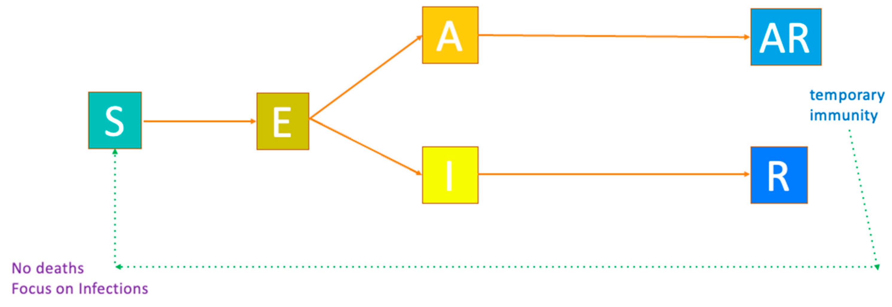
• The third realistic stochasticity presented in our model allows some exposed individuals to evolve to be asymptomatic, while the rest evolve to be infected (symptomatic). Both situations lead to immunity after some days (sweeps).

Figure 3. Two 3 × 3 lattices of nodes (a,b) representing populations. Arrows represent the possible contagions. Green arrows represent contacts that will lead to contagion. Red arrows represent contacts that will not lead to contagion. (a) both interactions lead to infections. (b) one of them is already infected so only the other interaction leads to a new infection.

Figure 3. Two 3 × 3 lattices of nodes (a,b) representing populations. Arrows represent the possible contagions. Green arrows represent contacts that will lead to contagion. Red arrows represent contacts that will not lead to contagion. (a) both interactions lead to infections. (b) one of them is already infected so only the other interaction leads to a new infection.

Finally, having tested a lot of scenarios and models, we ended up with a better structured model, which works as follows. Contagious individuals are divided into infected (I) and asymptomatic (A). Susceptible (S) individuals might become exposed (E) when they contact infected or asymptomatic individuals. After an incubation period, exposed individuals become infectious–contagious. Some of them are symptomatic (infected), while others are asymptomatic. Infected and asymptomatic individuals move to removed (R) and asymptomatic removed (AR), respectively, obtaining immunity. In this version of the model, we excluded deaths for simplicity.

Based on the flow diagram of the compartmental model suggested in [6], Figure 4 is a flow diagram of our compartmental model. For readers’ convenience, we use the same colors as in the simulation videos.

All of the above stochastic elements allow different paths to occur with the same initial conditions. This is one of the most important facts that makes this model a useful tool and offers an additive value to the existing literature.

2.2. Algorithm and Experimentation

We started exploring the potential of our model, using MATLAB [12]. We initially based our research on the model of [9], so we used a lattice of nodes, representing a population of individuals. We transformed it in a way that it could:

• become able to estimate the number of infected and susceptible individuals and represent those states clearly, by replacing charge with flag values. We used 1 for infected and 0 for susceptible. Diffusion of charge is replaced by contagion of virus to neighboring nodes/individuals,
• apply to an extended SIR model (we experimented using SEAIR). In addition to values 1 and 0, for infected (I) and susceptible (S), respectively, we used 0.5 for exposed (E), 0.75 for asymptomatic (A) and −0.25 and −0.5 for asymptomatic who recovered (AR) and infected who recovered (R), respectively,
• visualize results. Our model’s results can be depicted in short videos, presenting the lattice from day one (initial condition) to the final day. An observer can identify the exact coordinates of each infection and recovery and understand patterns of contagion and immunity building in the population.

According to the process we follow, after defining the size of the lattice, the parameters, and the initial conditions, the main steps are the following:

• All nodes/individuals are considered as susceptible. Then, according to the initial conditions, an amount of I₀, E₀, and A₀ nodes turn into infected, exposed and asymptomatic. Their positions are chosen through a random process (thus any repetition of the experiment is different).
• During the first step (period one):

  ○

  The algorithm recognizes all infected nodes/individuals and chooses randomly n out of 4 neighboring nodes as possible infectious connections. If any of the nodes chosen are susceptible, they may transform to exposed with a probability p that allows us to reproduce n × p infectious contacts per individual per period. If the nodes chosen are not susceptible, nothing changes.

  ○

  The same process with different parameters holds for asymptomatic nodes/individuals.

  ○

  The algorithm recognizes exposed nodes and may transform them into asymptomatic or infected. The exact period and the type of transformation are defined by a stochastic process, according to the parameters.

  ○

  The algorithm recognizes asymptomatic nodes and may transform them into asymptomatic recovered if the period of asymptomatic infection is completed.

  ○

  The algorithm recognizes infected nodes and may transform them into recovered if the period of symptomatic infection is completed.

  ○

  The algorithm recognizes immunized (asymptomatic recovered and recovered) nodes/individuals and may transform them into susceptible if the immunity period is completed.

• The process is repeated for all following periods, keeping track of the data.

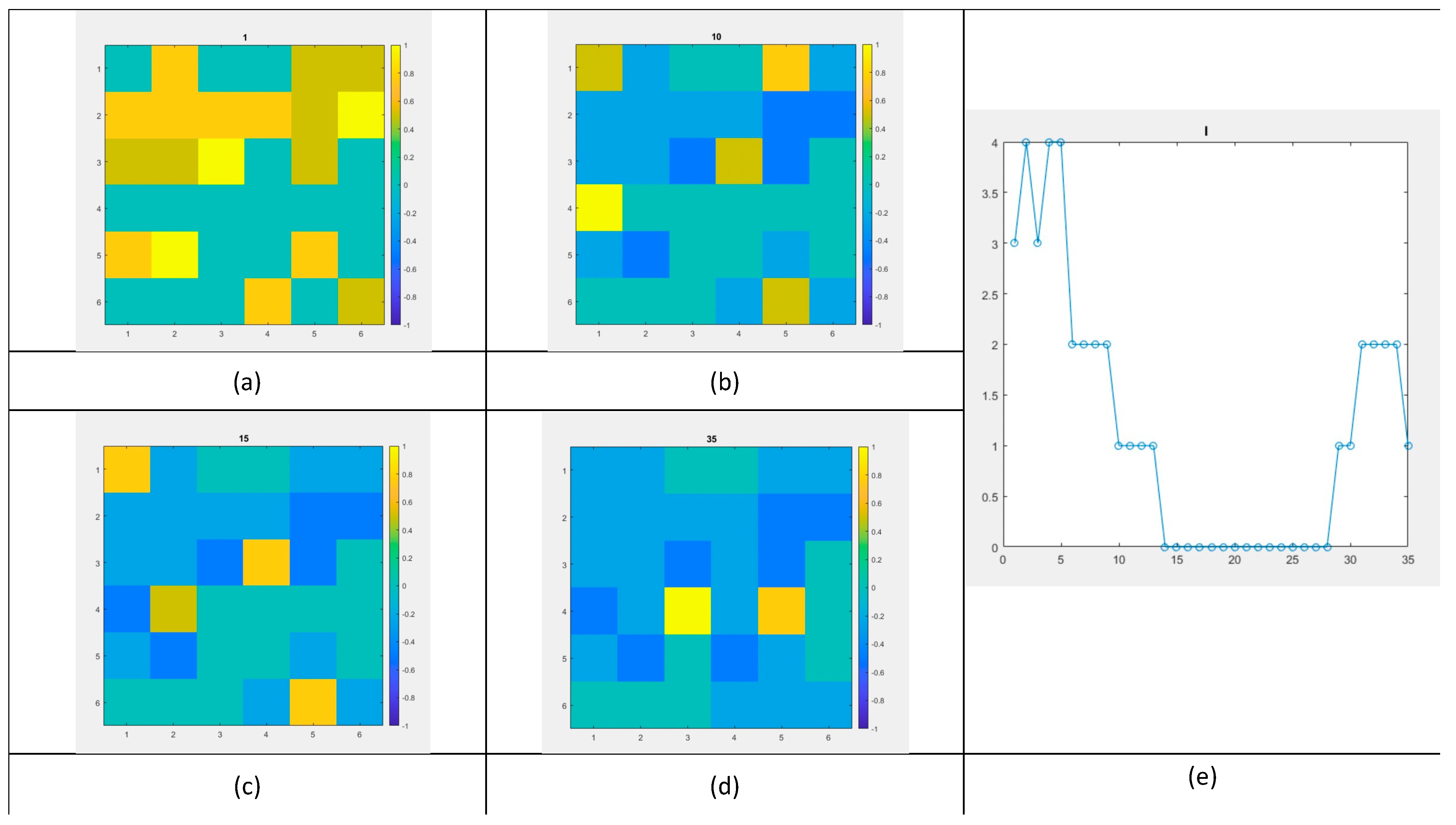
Our initial approach was focused on small lattices. An interesting size that is small but representative of the properties of our model is the 6 × 6 lattice. We present here two different cases, both starting with three infected individuals, in different places on the lattice. We observe its evolution for 120 days. Even if the lattice is small, the difference of the paths is obvious. 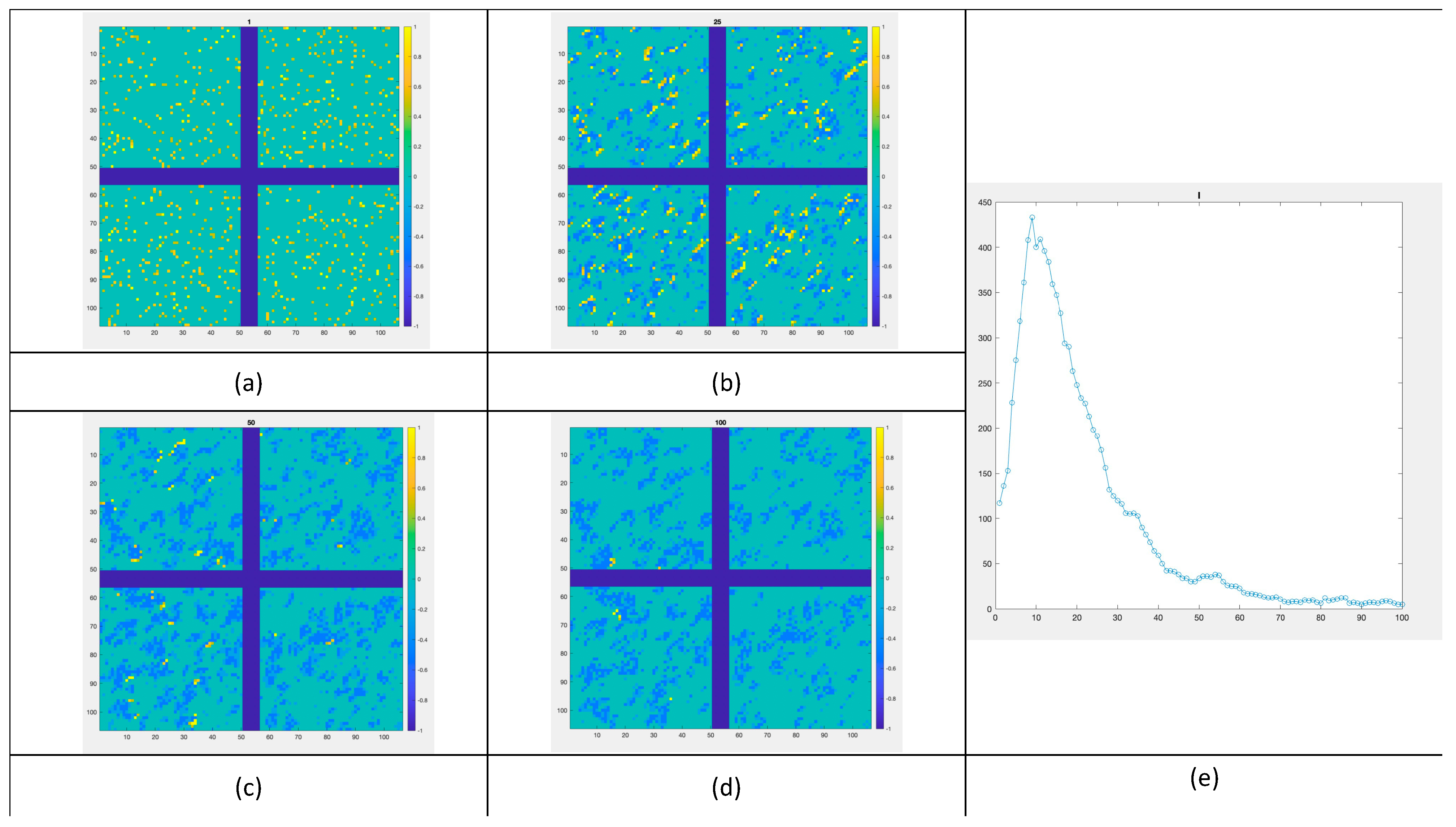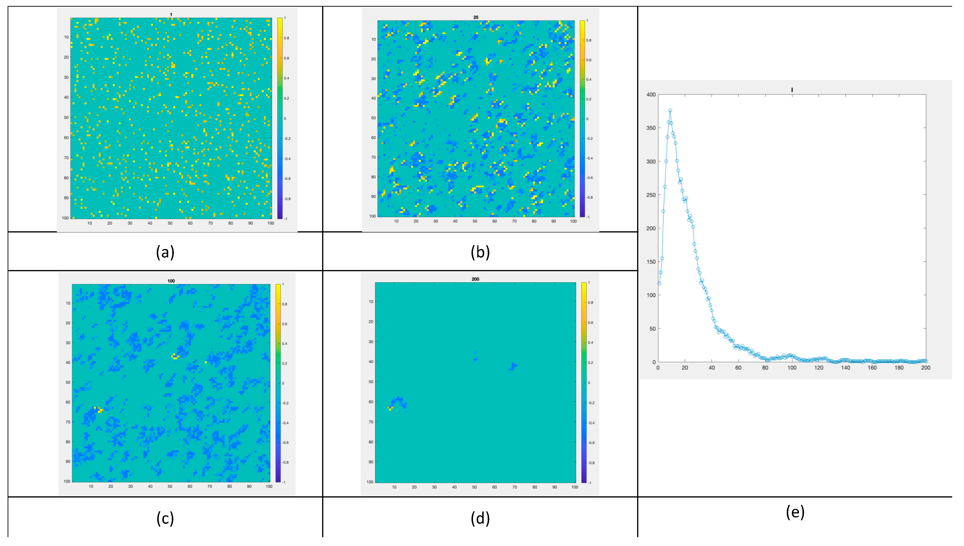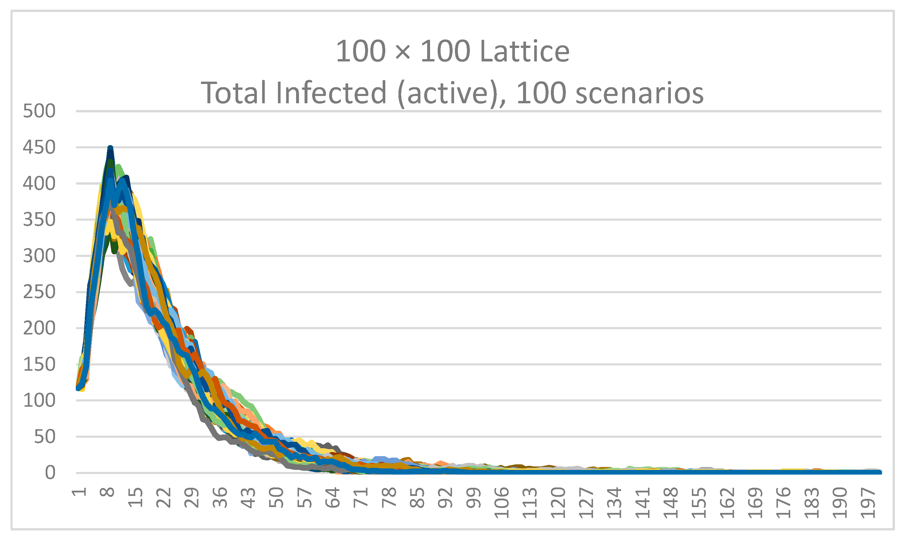Then we apply our model on a 100 × 100 lattice starting with 117 infected individuals for 200 days and we extensively analyze the results and insights that can be extracted.

Even though we have just been experimenting, we used parameters based (approximately) on the results of COVID-19 in Greece during the first months of its outbreak, in 2020 [7]. It became clear that those parameters should be corrected for our model, since we have to consider that new infections in each period are neighboring to old ones, leading to an important reduction of the effective reproductive number implied. At this point, we ignored hospitalization and death, considering that disease ended in recovery and immunization. We considered that this immunity effect lasts for 90 days, according to the relevant certificate that the Greek government issued initially [13]. The parameters we used are presented in

Table 1. Parameters and Initial Conditions (for Exposed, E₀, for Asymptomatic, A₀ and Infected, I₀) used in our Experimentation.

Parameter	Value Used
Recovery time (in days)	6
Immunity duration (in days)	90
Transmission rate (per infected)	0.31
Transmission rate (per asymptomatic)	0.21
Latent period (E → A) (in days)	3
Incubation period (E → I) (in days)	5
$E_0/I_0$	2.65
$A_0/I_0$	2.84

.

Finally, we tried to approximate the Greek population (10,768,477 individuals), by a square lattice of 3282 × 3282 dimensions. In this case we used the initial condition of 117 infected individuals (as on 12 March 2020, according to [7]) and tracked its evolution for 1000 days (up to 7 December 2022). The data are—reasonably—not fitting reality, since we have not applied any measures such as quarantine, mobility restrictions or vaccination.

3. Results

We used our model to estimate and visualize three different populations, using a 6 × 6 lattice, a 100 × 100 lattice and a 3282 × 3282 lattice. Having researched a wide variety of lattices of different sizes, it seems that there are finite-size effects that can affect reliability of the simulations. Larger lattices seem to provide more realistic simulations, reducing the finite-size effects [14]. We focused on the second one to extract and present the insights that can be obtained by applying this model. We suggest that our model is especially appropriate to identify a confidence interval for the evolution of the spread of a virus in a population. It can also reveal extraordinary but possible scenarios, based on any given initial conditions and parameters.

3.1. 6 × 6 Lattice

We use this relatively small and simple infrastructure to briefly explain the mechanisms and properties used in the model we created. In this presentation we have created two videos that use the same parameters and initial conditions, although the stochastic nature of our simulations allows for differences in the contagion and immunization process.

We observe that both Figure 5 (Video S1) and Figure 6 (Video S2) start having $I_0=3$, $E_0=7$ and $A_0=8$. Parameters are the same for both videos. In Figure 5 (Video S1), infected individuals increase fast. This reaches up to 9 individuals simultaneously. After day 20, the virus disappears. In Figure 6 (Video S2) we observe a maximum number of infected individuals equal to 4. It takes more than 35 days to reach zero cases. These important observed differences are strong arguments that support the use of our model to analyze the evolution of epidemics in populations.

A different scenario, using the same parameters and initial conditions, is presented in Figure 6 (Video S2). While at around 20 days, infected individuals are zero, on day 35 there are still asymptomatic and infected individuals. Obviously, exposed and asymptomatic individuals carried the virus and became contagious.

3.2. 100 × 100 Lattice

In larger lattices of more nodes, such as 100 × 100, differences become more clear and wider. The following two videos, Figure 7 (Video S3) and Figure 8 (Video S4), depict the paths of two populations with an initial “seeding” of 117 infected cases in different initial positions. We observed those populations for 200 days.

Again, there is an important difference in the number of days passed before the virus stops spreading and a difference in the height of the peaks of infected individuals. In Figure 7, there are very few infected individuals remaining after 100 days.

In Figure 8 (Video S4), we depict the differences that can appear when the initially infected individuals are in different places in the lattice. There are still many infected individuals after 100 days and some nodes are active even after 200 days. In Figure 8e we can identify separate waves of activity.

In Figure 7 (Video S3), infected individuals increase fast, reaching a maximum of more than 400 individuals, simultaneously, in less than 20 days. Before day 100, the virus has disappeared. In Figure 8 (Video S4) we observed a maximum number of infected individuals below 400 individuals. After 200 days, there are still a few infected individuals. Again, we claim that those different paths cannot be observed or even identified without a simulation model that accounts for realistic stochastic processes that affect the evolution of the system.

After running 100 different scenarios of the initial distribution of the 117 infected individuals, we can observe that the paths clearly follow a specific pattern, but differences are not so insignificant as to be ignored. Having the same number of initially infected individuals, placed on the same lattice, we observed that the maximum number of simultaneously infected individuals varies between 340 and 450 cases, representing more than 25% fluctuation, only after running 100 simulations. The time series of estimated infected individuals for 100 scenarios is presented in Figure 9.

Figure 9 makes clear that stochasticity plays a significant role in this procedure, and it should be considered while planning best response policies. An important difference that appeared is that the same initial conditions led most trajectories to one wave of the epidemic, while others included an additional, second, less intense wave. Especially in Video S4, we can observe endemic behavior of the virus spread.

To better present the utilities of our model, we found it useful to depict in Figure 10 the histogram of maximum infected individuals (at the same time) in all 100 scenarios.

This information allows policy makers to identify the probability of scenarios that exceed specific tolerance thresholds. For example, we can demonstrate that the estimated probability of having a peak of above 438 infected individuals is less than 4%.

3.3. 3282 × 3282 Lattice

Moving to a larger and more representative lattice of a country’s population, we used a 3282 × 3282 lattice. The number of its nodes is almost equal to the Greek population. Using 117 infected people (12 March 2020) as the initial condition in various places, we observed different results. We observed those populations for 1000 days. In Figure 11 (Video S5), we depict a representative case.

The capacity of this population allows for an extremely different path, compared to the case of the 100 × 100 lattice, although I₀ = 117 was still the initial condition. Observing the image of the lattice on the first day in this case, the 117 infected individuals are almost impossible to identify. Soon, contagion creates clusters of infected and recovered individuals, unveiling the location of the initial cases. After 1000 days, without intervention (restrictions, measures, vaccination) the number of active infected individuals is increasing rapidly, reaching 120,000.

3.4. Applying Borders

An interesting addition would be borders that separate the population into distinct regions that cannot communicate. This is an application that could describe the mobility restrictions among countries and regions.

In Figure 12 (Video S6), we observe a 100 × 100 lattice separated into four regions that cannot communicate. The results appear to support the effectiveness of such restrictions in mobility, as they appear to reduce the maximum number of infected individuals. More extensive separation in 9 or 16 regions seems to have even better effects on the results, reducing contagion effectively.

4. Discussion

Our multiple observations suggest that this way of modeling and visualizing the spread of COVID-19 can be helpful in understanding the range of different paths arising from the same initial conditions. We do not claim that this approach must replace traditional SIR models, but we suggest that it contributes to a better understanding of stochasticity, while it allows researchers to define proper probabilities on different paths, emerging from the same initial conditions, using a sufficiently large number of simulations. We have created a large number of computer simulations (realizations) to extract probability functions and observe rare events, according to the Monte Carlo method [15].

Since the data on the accurate location and interconnections of infected individuals are rarely available, SIR based models (like [6]) remain useful, but multiple simulations using our model allow the researchers to obtain a wider and more inclusive perspective on the situation. Figure 9 and Figure 10 in particular provide information that the existing literature ignores, namely the distribution of various possible outcomes under a determined set of parameters and initial conditions.

Compared to the SODM model, suggested by [9], our model allows for nodes being in more states than infected and susceptible, while it is easier to understand, as the nodes maintain agent-based model characteristics. As our model considers a more realistic way of contagion, we consider it provides a more extensive and natural view of the transmission process.

In a quite similar approach by [16], an agent-based model that describes COVID-19 transmission within facilities uses a model that allows for agents of two states (susceptible and infected). Our approach extends to more states (exposed, asymptomatic, recovered). Additionally, while [16] focuses on the effects of individuals’ density in facilities, our model considers a uniform density as all nodes have stable and equidistant positions on the lattice. As our nodes (agents) have fixed places on the lattice and permanent neighbors, our model seems to fit better the description of larger populations, such as regions or countries. Additionally, this stable structure allows us to focus our computational power on different states of the nodes (i.e., exposed, asymptomatic) and random contacts (and contagion) between neighboring nodes.

We also suggest that the visualization of the forecasted paths can allow audiences who are not familiar with virus spread to better understand the situation and the reasons leading to any measures applied. Our work provides a MATLAB-2020 code (ver. 9.9.0) (Appendix A) that allows anyone to recreate, visualize and observe the whole map of all agents for separate simulations. As [17] explains, agent-based models are better learning tools, rather than predicting because their perspective is more natural. Our model is motivated by this purpose and we consider it allows for this exact use.

Our future steps include the application of this model on COVID-19 spread and vaccination in Greece, with an emphasis on the small islands of Greece, where location and (almost natural) isolation of small populations makes such simulations very useful to understand the dynamics of epidemics.

5. Conclusions

In this research, we present a tool that can successfully simulate and visualize the diffusion of contagious diseases through populations. We mainly focused on COVID-19, although the model could be applied to any contagious disease, if adjusted appropriately.

We observed that the size of the population lattice and the specific location of the initially infected individuals in the population lattice is critical to the evolution and the spread of infections. The duration, the intensity of the pandemic and the number of waves seem to extensively depend on those initial conditions, a property that is fundamentally ignored by the SIR and extended SIR models.

We suggest a method that allows interested parties to understand and better explain the probabilities of different scenarios and, thus, improve the ways to predict and prevent the expansion of spreading diseases and viruses. The insights provided could become a useful tool to investigate and compare different policies and understand the importance of implementing any measures.

Visualization of the results might become a useful tool to explain and communicate the diffusion of infections through a population to less familiar audiences, convincing them to act in accordance with any given situation and prevent unhealthy behaviors or overreacting.

References

- World Health Organization. Coronavirus Disease (COVID-19). Available online: https://www.who.int/emergencies/diseases/novel-coronavirus-2019 (accessed on 30 June 2023).
- Kermack, W.O.; McKendrick, A.G. A contribution to the mathematical theory of epidemics. Proc. R. Soc. Lond. Ser. A 1927, 115, 700–721. [Google Scholar] [CrossRef]
- Lajmanovich, A.; Yorke, J.A. A deterministic model for gonorrhea in a nonhomogeneous population. Math. Biosci. 1976, 28, 221–236. [Google Scholar] [CrossRef]
- Nallaswamy, R.; Shukla, J.B. Effects of dispersal on the stability of a gonorrhea endemic model. Math. Biosci. 1982, 61, 63–72. [Google Scholar] [CrossRef]
- Allen, L.J.; Kirupaharan, N.; Wilson, S.M. SIS epidemic models with multiple pathogen strains. J. Differ. Equ. Appl. 2004, 10, 53–75. [Google Scholar] [CrossRef]
- Xia, Z.Q.; Zhang, J.; Xue, Y.K.; Sun, G.Q.; Jin, Z. Modeling the transmission of Middle East respirator syndrome corona virus in the Republic of Korea. PLoS ONE 2015, 10, e0144778. [Google Scholar] [CrossRef] [PubMed]
- Kevrekidis, P.G.; Cuevas-Maraver, J.; Drossinos, Y.; Rapti, Z.; Kevrekidis, G.A. Reaction-diffusion spatial modeling of COVID-19: Greece and Andalusia as case examples. Physical Rev. E 2021, 104, 024412. [Google Scholar] [CrossRef] [PubMed]
- Singh, A.; Deolia, P. COVID-19 outbreak: A predictive mathematical study incorporating shedding effect. J. Appl. Math. Comput. 2022, 69, 1239–1268. [Google Scholar] [CrossRef] [PubMed]
- Contoyiannis, Y.; Stavrinides, S.G.P.; Hanias, M.; Kampitakis, M.; Papadopoulos, P.; Picos, R.; Potirakis, M.S. A Universal Physics-Based Model Describing COVID-19 Dynamics in Europe. Int. J. Environ. Res. Public Health 2020, 17, 6525. [Google Scholar] [CrossRef] [PubMed]
- Ramani, A.; Carstea, A.S.; Willox, R.; Grammaticos, B. Oscillating epidemics: A discrete-time model. Physica A 2004, 333, 278–292. [Google Scholar] [CrossRef]
- Kadelka, C. Projecting social contact matrices to populations stratified by binary attributes with known homophily. arXiv 2022, arXiv:2207.12328. [Google Scholar] [CrossRef] [PubMed]
- MATLAB, Version 9.9.0; The MathWorks Inc.: Natick, MA, USA, 2020.
- Greek Legislation Concerning “Emergency Measures to Protect Public Health from the Risk of Further Spread of the COVID-19 Coronavirus”, FEK 1099/11.03.2022, B. Available online: https://www.aade.gr/sites/default/files/2022-03/1099fek.pdf (accessed on 29 November 2023).
- Argyrakis, P.; Kopelman, R.; Lindenberg, K. Diffusion-limited binary reactions: The hierarchy of nonclassical regimes for random initial conditions. Chem. Phys. 1993, 177, 693–707. [Google Scholar] [CrossRef]
- Kroese, D.P.; Brereton, T.J.; Taimre, T.; Botev, Z.I. Why the Monte Carlo method is so important today. Wiley Interdiscip. Rev. Comput. Stat. 2014, 6, 386–392. [Google Scholar] [CrossRef]
- Cuevas, E. An agent-based model to evaluate the COVID-19 transmission risks in facilities. Comput. Biol. Med. 2020, 121, 103827. [Google Scholar] [CrossRef] [PubMed]
- Bonabeau, E. Agent-based modeling: Methods and techniques for simulating human systems. Proc. Natl. Acad. Sci. USA 2002, 99 (Suppl. S3), 7280–7287. [Google Scholar] [CrossRef] [PubMed]