Estimation of Expectations and Variance Components in Two-Level Nested Simulation Experiments

Abstract

When there is uncertainty in the value of parameters of the input random components of a stochastic simulation model, two-level nested simulation algorithms are used to estimate the expectation of performance variables of interest. In the outer level of the algorithm n observations are generated for the parameters, and in the inner level m observations of the simulation model are generated with the values of parameters fixed at the values generated in the outer level. In this article, we consider the case in which the observations at both levels of the algorithm are independent and show how the variance of the observations can be decomposed into the sum of a parametric variance and a stochastic variance. Next, we derive central limit theorems that allow us to compute asymptotic confidence intervals to assess the accuracy of the simulation-based estimators for the point forecast and the variance components. Under this framework, we derive analytical expressions for the point forecast and the variance components of a Bayesian model to forecast sporadic demand, and we use these expressions to illustrate the validity of our theoretical results by performing simulation experiments with this forecast model. We found that, given a fixed number of total observations $nm$, the choice of only one replication in the inner level ($m=1$) is recommended to obtain a more accurate estimator for the expectation of a performance variable.

1. Introduction and Notation

Simulation is usually regarded as a powerful tool for producing forecasts, evaluating risk (see, e.g., [1]), and animating and illustrating a system’s performance over time (see, e.g., [2]). When a component of a simulation model has a certain degree of uncertainty, it is said to be a random component, and it is modeled by using a probability distribution and/or a stochastic process that is sampled throughout the simulation run to produce a stochastic simulation. A random component typically depends on the value of certain parameters; we denote by $\theta$ a particular value for the vector of parameters of the random components of a stochastic simulation, and $\Theta$ denotes a random vector that corresponds to the parameter values when there is uncertainty in the values of these parameters.

Following the notation of [1], the output of a stochastic (dynamic) simulation can be regarded as a stochastic process $\left\{Y\right(s):s\ge 0;\Theta \}$, where $Y\left(s\right)$ is a random vector (of arbitrary dimension d) representing the state of the simulation at time $s\ge 0$. The term transient simulation applies to a dynamic simulation that has a well-defined termination time, so the output of a transient simulation can be viewed as a stochastic process $\left\{Y\right(s):0\le s\le T;\Theta \}$, where T is a stopping time (which may be deterministic); see, e.g., [3] for a definition of stopping time.

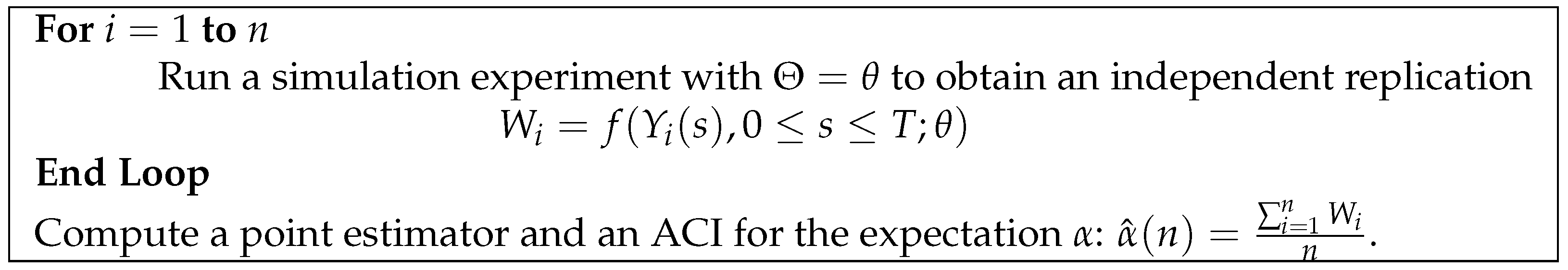
A performance variable W in a transient simulation is a real-valued random variable (r.v.) that depends on the simulation output up to time T, i.e., $W=f\left(Y\right(s),0\le s\le T;\Theta )$, and the expectation of a performance variable W is a performance measure that we usually estimate through experimentation with the simulation model. When there is no uncertainty in the parameters of the random components, the accepted technique for estimating a performance measure in transient simulation is the method of independent replications. This method consists of running experiments with the simulation model to produce n replications $W_1,W_2,\dots ,W_n$ that can be regarded as independent and identically distributed (i.i.d.) random variables (see Figure 1).

In the method of independent replications, a point estimator for the expectation $\alpha =E\left[W_1\right]$ is the average $\widehat{\alpha }\left(n\right)=\frac{{\sum }_{i=1}^n{W}_i}{n}$. If $E\left[\right|W_1\left|\right]<\infty$, it follows from the classical Law of Large Numbers (LLN) that $\widehat{\alpha }\left(n\right)$ is consistent, i.e., it satisfies $\widehat{\alpha }\left(n\right)\Rightarrow \alpha$, as $n\to \infty$ (where ⇒ denotes weak convergence of random variables); see, e.g., [3] for a proof. Consistency ensures that the estimator approaches the parameter as the number of replications n increases, and an asymptotic confidence interval (ACI) for the parameter is often used to evaluate the accuracy of the simulation-based estimator. Typically, a Central Limit Theorem (CLT) for the estimator is used to derive the expression for an ACI (see, for example, chapter 3 of [4]). For the case of the expectation $\alpha$ in the algorithm of Figure 1, if $E\left[W_1^2\right]<\infty$, the classical CLT implies that

$$\frac{\sqrt{n}(\widehat{\alpha }\left(n\right)-\alpha )}{\sigma }\Rightarrow N(0,1),$$

(1)

as $n\to \infty$, where ${\sigma }^2=E\left[{(W_1-\alpha )}^2\right]$, and $N(0,1)$ denotes an r.v. distributed as normal with a mean of 0 and variance of 1. Then, if $E\left[W_1^2\right]<\infty$, it follows from (1) and Slutsky’s Theorem (see Appendix A) that

$$\frac{\sqrt{n}(\widehat{\alpha }\left(n\right)-\alpha )}{\widehat{\sigma }\left(n\right)}\Rightarrow N(0,1),$$

as $n\to \infty$, where $\widehat{\sigma }\left(n\right)$ denotes the sample standard deviation, i.e., ${\widehat{\sigma }}^2\left(n\right)=\frac{{\sum }_{i=1}^n{(W_i-\widehat{\alpha }\left(n\right))}^2}{n-1}$. This CLT implies that

$$\underset{n\to \infty }{lim}P[\left|\widehat{\alpha }\left(n\right)-\alpha \right|\le z_{\beta }\widehat{\sigma }\left(n\right)/\sqrt{n}]=1-\beta ,$$

for $0<\beta <1$, where $z_{\beta }$ is the ($1-\beta /2$)-quantile of a $N(0,1)$, so the CLT of Equation (2) is sufficient to establish a $100(1-\beta )\%$ ACI for $\alpha$ with the following halfwidth:

$$H{W}_{\alpha }=z_{\beta }\widehat{\sigma }\left(n\right)/\sqrt{n}.$$

(2)

The standard measurement used in simulation software (e.g., Simio; see [2]) to evaluate the accuracy of $\widehat{\alpha }\left(n\right)$ as an estimator of expectation $\alpha$ is a halfwidth in the form of (2).

The parameters of the random input components of a simulation model are typically estimated from real-data observations (denoted by a real-valued vector x), in contrast to an estimation of output performance measures that uses observations from simulation experiments. While the majority of applications covered in the related literature assume that there is no uncertainty in the value of input parameters, the uncertainty can be significant when these parameters are estimated by using small amounts of data. In these situations, Bayesian statistics can be used to incorporate this uncertainty in the output analysis of simulation experiments via the use of a posterior distribution $p\left(\theta \right|x)$. 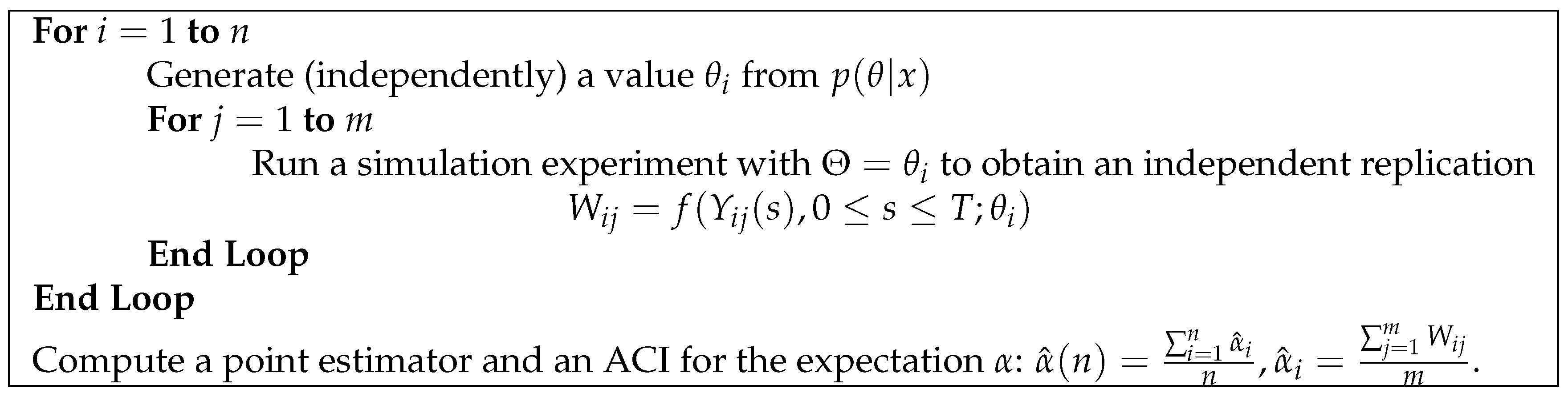A two-level nested simulation algorithm (see, e.g., [5,6,7]) is a methodology that is currently proposed for the analysis of simulation experiments under parameter uncertainty. In the outer level, we simulate n observations for the parameters from a posterior distribution $p\left(\theta \right|x)$, while in the inner level, we simulate m observations for the performance variable with the parameters fixed at the value $\theta$ generated in the outer level. In this paper, we focus on the case where the observations at both levels of the algorithm are independent (as illustrated in Figure 2). We first show how the variance of a simulated observation can be decomposed into parametric and stochastic variance components, and then we obtain CLTs for the estimator of the point forecast and the estimators of the variance components. Our CLTs allow us to compute an ACI for each estimator. Our results are validated through experiments with a forecast model for sporadic demand reported in [8]. The main theoretical results reported in this paper were first stated in [9] (although the proofs were omitted), and in this paper, we provide the missing proofs, a more comprehensive literature review, and a more complete set of experiments with different values for the parameters of our experiments.

The existing literature on quantifying the impact of uncertainty on the input components of a stochastic simulation is very extensive; detailed reviews can be found, e.g., in [10,11,12] and the references therein. However, in order to situate our results within the framework of the bibliography related to the input analysis of simulation experiments, next, we present a brief discussion of the different approaches that have been proposed on this topic.

According to Barton et al. [13], input analysis in the simulation literature has been addressed essentially in two ways: sensitivity analysis and the characterization of the impact of input uncertainty to provide an ACI (to evaluate the accuracy of a point estimator) that explicitly considers this uncertainty. A sensitivity analysis is performed by running simulation experiments under different distributions for the random components and/or different parameters in order to investigate and describe the changes in the main performance measures of the simulation experiments (see [14,15] for early proposals). Although formalization of this approach was initially proposed by using techniques (e.g., design of experiments and/or regression; see [16]) that were previously proposed to analyze real-world experiments (see, e.g., [17]), some other techniques were proposed for the special purpose of simulation; for example, Freimer and Schruben [18] discussed methods for the design of experiments to search for the sample size of input data that ensured that the difference in the results of two simulation experiments was dominated by the stochastic variance (induced by the simulation experiments) so that the parametric variance (induced by input uncertainty) was not significant for decision making. As pointed out by Bruce Schmeiser in his discussion in [19], sensitivity analysis has a wide range of applications, since it can handle model uncertainty, as well as situations where no real-world data exist; however, a significant drawback is that it does not provide a statistical characterization of input uncertainty. This characterization can be achieved through the construction of an ACI that explicitly considers input uncertainty based on sample data.

According to several authors (e.g., [10,13]), for the construction of an ACI that explicitly considers the impact of input uncertainty, there have been essentially three approaches: the delta method, resampling, and Bayesian methods. Let us denote by $\eta \left(\theta \right)$ the expectation of $W_1$ (of Figure 1) as a function of $\theta$, and let ${\widehat{\theta }}_r$ be an estimator for parameter $\theta$ (where r is the sample size of real-world observations); in this notation, the main idea of the delta method is to consider a Taylor series expansion for $\eta \left({\widehat{\theta }}_r\right)$ around $\theta$ to investigate convergence properties (as $r\to \infty$) of $\eta \left({\widehat{\theta }}_r\right)$ as an estimator of $\eta \left(\theta \right)$. Cheng and Holland ([20,21,22]) introduced the use of the delta method to propose the construction of confidence intervals for the expectation of a performance variable of a stochastic simulation under uncertainty in the parameters of a proposed (known) parametric family of distributions for a random component. In [20,22], the authors did not formally prove the asymptotic validity of their proposed confidence intervals but justified them by appealing to the asymptotic normality (as $r\to \infty$) of the estimator ${\widehat{\theta }}_r$ (which is the case, under regularity conditions, when ${\widehat{\theta }}_r$ is the maximum likelihood estimator). In a later publication ([23]), Cheng and Holland provided proof of the asymptotic validity of their confidence intervals based on the delta method under regularity conditions as $r\to \infty$ and $n\to \infty$. In [20,23], the authors also proposed the construction of asymptotic confidence intervals under parameter uncertainty based on a resampling technique known as parametric bootstrapping; this proposal basically consisted of using the algorithm of Figure 1 but sampling the values for parameter $\theta$ from the likelihood evaluated at the maximum likelihood estimator. Some other proposals for the construction of an ACI are based on resampling from the empirical distribution of real-data observations (see, e.g., [13,24,25]). A drawback of proposed confidence intervals based on the delta method and resampling is that their asymptotic validity (see the Theorem of [23] and Theorem 1 of [13]) requires that the sample size of real observations be large ($r\to \infty$), which is a condition that is probably true for big data, in which case parameter uncertainty may not be significant. Another drawback of techniques based on the delta method and parametric bootstrapping is that parameter $\theta$ is assumed to be deterministic (although unknown) so that, at some point, the value of $\theta$ is replaced by $\widehat{\theta }$, and this is one reason for why these methods are called frequentists in the statistics community. On the contrary, under a Bayesian approach, a parameter is regarded as a random variable $\Theta$, and the uncertainty about $\Theta$ is assessed through a posterior distribution $p\left(\theta \right|x)$ that explicitly incorporates available information from sample data x.

Bayesian methods have solid theoretical foundations (see, e.g., [26]), and they have been proposed to assess not only parameter uncertainty, but also model uncertainty (see [27]). Bayesian methods for input analysis in simulation experiments were introduced by Chick in [28], and since then, there has been a fair number of publications on Bayesian methods for input simulation analysis (see, e.g., [7,29,30,31]). Bayesian methods require the specification of a prior distribution on the input parameters of the simulation model, and some users object to this requirement; however, there is a well-developed theory on objective priors (see, e.g., [32]), and some authors (e.g., [10,33]) consider that this requirement is actually a strength of the approach. Another strength of Bayesian methods for input analysis in stochastic simulation is that some Bayesian methods have been developed to construct an ACI for parameters that are not the expectation—for example, the variance and quantiles for a consistent estimation of a credible interval for the performance variable W (see [34]). It is worth mentioning that some methods need the extra assumption that the simulation output satisfies a meta-model in order to justify the asymptotic validity of their proposed confidence intervals (e.g., [13,35]); as we will see, this extra assumption is not required to establish an ACI for the expectation and variance components of two-level simulation experiments in a Bayesian framework.

The organization of this article is as follows. After this introduction, our proposed methodologies for the computation of an ACI for the point forecast and the variance components in a two-level simulation experiment are then described, and the mathematical results that support the validity of the proposed ACIs are stated (the corresponding proofs are provided in Appendix A). In the next section, we illustrate our notation by obtaining the analytical solutions for the point forecast and the variance components of a Bayesian model to forecast sporadic demand. This solution is used in the next section to illustrate and support, through simulation experiments, the validity of the ACIs proposed in this article. In the final section, we summarize our findings and suggestions for future research.

2. Theoretical Results

To identify the parameters that we wish to estimate by using the two-level nested algorithm in Figure 2, we denote $\mu (\Theta )\stackrel{def}{=}E\left[W_{11}\right|\Theta ]$, and ${\sigma }^2(\Theta )\stackrel{def}{=}E\left[W_{11}^2\right|\Theta ]-{\mu }^2(\Theta )$. In this notation, the point forecast is the expectation $\alpha =E\left[\mu \right(\Theta \left)\right]$, and the variance of each $W_{ij}$ is:

$$V\left[W_{ij}\right]\stackrel{def}{=}E\left[W_{ij}^2\right]-E{\left[W_{ij}\right]}^2=E[E\left[W_{ij}^2\right|\Theta ]-\mu {(\Theta )}^2]+E\left[\mu {(\Theta )}^2\right]-E{\left[\mu (\Theta )\right]}^2={\sigma }_S^2+{\sigma }_P^2,$$

(3)

for $i=1,\dots ,n$; $j=1,\dots ,m$, where ${\sigma }_P^2=V\left[\mu (\Theta )\right]\stackrel{def}{=}E\left[\mu {(\Theta )}^2\right]-E{\left[\mu (\Theta )\right]}^2$, and ${\sigma }_S^2=E\left[{\sigma }^2(\Theta )\right]$, where ${\sigma }^2(\Theta )$ was previously defined. We mention that, in the relevant literature, ${\sigma }_S^2$ is usually referred to as stochastic variance, and ${\sigma }_P^2$ is usually referred to as parametric variance.

2.1. Point Estimators

In this paper, we are interested in both the estimation of the point forecast $\alpha =E\left[\mu \right(\Theta \left)\right]$ and the estimators of the variance components of every observation generated in the algorithm in Figure 2 and defined in (3); thus, we first consider the natural point estimators

$$\widehat{\alpha }\left(n\right)=\frac{1}{n}\sum _{i=1}^n{\widehat{\alpha }}_i,{\widehat{\sigma }}_T^2\left(n\right)=\frac{1}{n-1}\sum _{i=1}^n{({\widehat{\alpha }}_i-\widehat{\alpha }\left(n\right))}^2,{\widehat{\sigma }}_S^2\left(n\right)=\frac{1}{n}\sum _{i=1}^n{S}_i^2,$$

(4)

where ${\widehat{\alpha }}_i=m^{-1}{\sum }_{j=1}^m{W}_{ij}$, and $S_i^2={(m-1)}^{-1}{\sum }_{j=1}^m{(W_{ij}-{\widehat{\alpha }}_i)}^2$, $i=1,\dots ,m$. Note that the ${\widehat{\alpha }}_i$s are i.i.d. with expectation $E\left[{\widehat{\alpha }}_1\right]=\alpha$ and variance

$$\begin{array}{ccc}\hfill {\sigma }_T^2& \stackrel{def}{=}& E\left[{({\widehat{\alpha }}_1-\alpha )}^2\right]=m^{-2}(mE\left[{(W_{11}-\alpha )}^2\right]+m(m-1)E\left[(W_{11}-\alpha )(W_{12}-\alpha )\right])\hfill \\ & =& m^{-1}({\sigma }_S^2+{\sigma }_P^2)+m^{-1}(m-1){\sigma }_S^2={\sigma }_S^2+m^{-1}{\sigma }_P^2.\hfill \end{array}$$

(5)

In addition, note that the $S_i^2$ values are i.i.d. with expectation $E\left[S_1^2\right]={\sigma }_S^2$, $i=1,\dots ,n$. Thus, the next proposition follows from the classical LLN.

Proposition 1.

If $m\ge 1$ and $E\left[W_{11}^2\right]<\infty$, then $\widehat{\alpha }\left(n\right)$ and ${\widehat{\sigma }}_T^2\left(n\right)$ are unbiased and consistent (as $n\to \infty$) estimators for α and ${\sigma }_T^2$ (as defined in (5)), respectively.

Furthermore, if $m\ge 2$ and $E\left[W_{11}^2\right]<\infty$, then ${\widehat{\sigma }}_S^2\left(n\right)$ is an unbiased and consistent (as $n\to \infty$) estimator for ${\sigma }_S^2$ (as defined in (3)).

2.2. Accuracy of the Point Estimators

As we stated in Proposition 1, under mild assumptions, the point estimators proposed in (4) are consistent and, thus, converge to the corresponding parameter value (as $n\to \infty$). However, to determine the degree of accuracy of these estimators, we must establish a CLT for each estimator to derive a valid expression for the corresponding ACI. Note that both $\widehat{\alpha }\left(n\right)$ and ${\widehat{\sigma }}_S^2\left(n\right)$ are averages of i.i.d observations; thus, the next proposition follows from the classical CLT for i.i.d. observations.

Proposition 2.

If $m\ge 1$ and $E\left[W_{11}^2\right]<\infty$, then

$$\frac{\sqrt{n}(\widehat{\alpha }\left(n\right)-\alpha )}{{\sigma }_T}\Rightarrow N(0,1),$$

as $n\to \infty$.

  Furthermore, if $m\ge 2$ and $E\left[W_{11}^4\right]<\infty$, then

$$\frac{\sqrt{n}({\widehat{\sigma }}_S^2\left(n\right)-{\sigma }_S^2)}{\sqrt{V_S}}\Rightarrow N(0,1),$$

as $n\to \infty$, where ${\sigma }_S^2$ is defined in (3), ${\sigma }_T^2$ is defined in (5), $\widehat{\alpha }\left(n\right)$, ${\widehat{\sigma }}_S^2\left(n\right)$ are defined in (4), and $V_S=E\left[{(S_1^2-{\sigma }_S^2)}^2\right]$, where $S_1^2$ is defined in (4).

Since we have consistent estimators for ${\sigma }_T^2$ and $V_S$ (under mild assumptions), the next corollary follows from Proposition 1 and Slutsky’s Theorem; the details of the proof are given in Appendix A.

Corollary 1.

Under the same notation and assumptions as in Proposition 2, for $m\ge 1$, we have

$$\frac{\sqrt{n}(\widehat{\alpha }\left(n\right)-\alpha )}{\sqrt{{\widehat{\sigma }}_T^2\left(n\right)}}\Rightarrow N(0,1),$$

as $n\to \infty$, and for $m\ge 2$, we have

$$\frac{\sqrt{n}({\widehat{\sigma }}_S^2\left(n\right)-{\sigma }_S^2)}{\sqrt{{\widehat{V}}_S\left(n\right)}}\Rightarrow N(0,1),$$

as $n\to \infty$, where ${\widehat{\sigma }}_S^2\left(n\right)$ and ${\widehat{\sigma }}_T^2\left(n\right)$ are defined in (4), and

$$\widehat{V_s}\left(n\right)=\frac{1}{n-1}\sum _{i=1}^n{(S_i^2-S^2)}^2,S^2=\frac{1}{n}\sum _{i=1}^n{S}_i^2.$$

In order to obtain a CLT for ${\widehat{\sigma }}_T^2\left(n\right)$, note that this estimator is the sample variance of i.i.d. observations; thus we can use the following lemma. A proof using the delta method (see, e.g., Proposition 2 of [36] for a proof) is provided in Appendix A.

Lemma 1.

If $X_1,X_2,\dots$ is a sequence of i.i.d. random variables with $E\left[X_1^4\right]<\infty$, then

$$\frac{\sqrt{n}(S^2\left(n\right)-{\sigma }_1^2)}{\sqrt{{\sigma }_2^2}}\Rightarrow N(0,1),$$

as $n\to \infty$, where ${\sigma }_1^2={\mu }_2-{\mu }_1^2$, ${\sigma }_2^2={\mu }_1^2{\mu }_2-4{\mu }_1^4-4{\mu }_1{\mu }_3+{\mu }_4-{\mu }_2^2$, ${\mu }_k=E\left[X_1^k\right]$, $k=1,2,3,4$; $S^2\left(n\right)={(n-1)}^{-1}{\sum }_{i=1}^n{(X_i-{\widehat{\mu }}_1)}^2$, ${\widehat{\mu }}_1=n^{-1}{\sum }_{i=1}^n{X}_i$.

Note that, for $k=1,2,3,4$, ${\widehat{\mu }}_k$ of Lemma 1 is an unbiased and consistent estimator for ${\mu }_k$, so the next corollary follows directly from Lemma 1.

Corollary 2.

Under the same assumptions as those in Lemma 1, we have

$$\frac{\sqrt{n}(S^2\left(n\right)-{\sigma }_S^2)}{\sqrt{{\widehat{\sigma }}_2^2\left(n\right)}}\Rightarrow N(0,1),$$

as $n\to \infty$, where ${\widehat{\sigma }}_2^2=8{\widehat{\mu }}_1^2{\widehat{\mu }}_2-4{\widehat{\mu }}_1^4-4{\widehat{\mu }}_1{\widehat{\mu }}_3+{\widehat{\mu }}_4-{\widehat{\mu }}_2^2$, ${\widehat{\mu }}_k=n^{-1}{\sum }_{i=1}^n{X}_i^k$.

Since ${\widehat{\sigma }}_T^2\left(n\right)$ is the sample variance of ${\widehat{\alpha }}_i$, $i=1,\dots ,n$, the next corollary follows directly from Lemma 1.

Corollary 3.

If $m\ge 1$ and $E\left[W_{11}^4\right]<\infty$, then

$$\frac{\sqrt{n}({\widehat{\sigma }}_T^2\left(n\right)-{\sigma }_T^2)}{\sqrt{{\widehat{V}}_T\left(n\right)}}\Rightarrow N(0,1),$$

as $n\to \infty$, where ${\widehat{V}}_T\left(n\right)=8{\overline{\alpha }}_1^2{\overline{\alpha }}_2-4{\overline{\alpha }}_1^4-4{\overline{\alpha }}_1{\overline{\alpha }}_3+{\overline{\alpha }}_4-{\overline{\alpha }}_2^2$, ${\overline{\alpha }}_k=n^{-1}{\sum }_{i=1}^n{\widehat{\alpha }}_i^k$, $k=1,2,3,4$.

Corollaries 1, 2, and 3 are the CLTs required to establish an ACI for the point forecast $\alpha$, the stochastic variance ${\sigma }_S^2$, and the variance ${\sigma }_T^2={\sigma }_S^2+m^{-1}{\sigma }_P^2$, respectively. According to these corollaries, for $0<\beta <1$, the $100(1-\beta )\%$ ACIs are centered in the corresponding point estimator, and have halfwidths are given by:

$$H{W}_{\alpha }=z_{\beta }\frac{\sqrt{{\widehat{\sigma }}_T^2\left(n\right)}}{\sqrt{n}},H{W}_{{\sigma }_S^2}=z_{\beta }\frac{\sqrt{{\widehat{V}}_S\left(n\right)}}{\sqrt{n}},\mathrm{and}H{W}_{{\sigma }_T^2}=z_{\beta }\frac{\sqrt{{\widehat{V}}_T\left(n\right)}}{\sqrt{n}},$$

(6)

for $\alpha$, ${\sigma }_S^2$, and ${\sigma }_T^2$, respectively, where ${\widehat{\sigma }}_T^2\left(n\right)$ is defined in (4), and ${\widehat{V}}_S\left(n\right)$ and ${\widehat{V}}_T\left(n\right)$ are defined in Corollary 1 and in Corollary 3, respectively.

As we have seen, by using the algorithm in Figure 2, we can build valid ACIs for the parameters of interest in this article, although a relevant question is that of how to distribute the computing time between the two loops to obtain more accurate point estimators—that is, given a budget $k=nm$, which value of m provides the most accurate estimators? For the case of the estimation of the point forecast $\alpha$, we can answer this question, as we explain below. Since the point estimator $\widehat{\alpha }\left(n\right)$ is an average of i.i.d. random variables, for fixed values of $k=nm$, it follows from Equation (5) that the variance of $\widehat{\alpha }\left(n\right)$ is given by

$$n^{-1}{\sigma }_T^2=k^{-1}(m{\sigma }_S^2+{\sigma }_P^2),$$

(7)

and takes its minimal value when $m=1$, suggesting that the point estimator $\widehat{\alpha }\left(n\right)$ defined in (4) is more accurate when m is smaller (i.e., it takes the value of 1). However, note that a smaller value of m is convenient (from the point of view of running time) for a fixed budget of $k=nm$ when the computing time needed to generate a random variate from $p\left(\theta \right|x)$ in the algorithm in Figure 2 is negligible compared to the computing time needed to generate $W_{ij}$, as is the case in most real applications.

Note that the TLCs stated in Xorollaries 1, 2 and 3 were obtained for a fixed value of m as $n\to \infty$ in the algorithm in Figure 2, which means that the accuracy of the corresponding point estimator increases as the number of observations in the outer level increases and m remains fixed. An interesting result is that we can also obtain a TLC for the point forecast $\alpha$ if we allow m to increase with n, as we state in the following proposition (a proof using the Lindeberg–Feller theorem is provided in Appendix A).

Proposition 3.

Given $0<p\le 1$, if $m=\lfloor n^{-1+1/p}\rfloor$ and $E\left[W_{11}^2\right]<\infty$, then

$$\frac{\sqrt{n}(\widehat{\alpha }\left(n\right)-\alpha )}{\sqrt{{\sigma }_T^2}}\Rightarrow N(0,1),$$

as $n\to \infty$, where ${\sigma }_T^2$ is defined in (5) and, for any real number s, $\lfloor s\rfloor$ denotes the integer part of s.

Note that the last proposition implies that the ACI defined in Equation (6) for the point forecast $\alpha$ is also valid under the assumptions of Proposition 3. If, once again, we set the total number of iterations in the algorithm in Figure 2 to $k=nm$, we let $n\approx k^p$, $m\approx k^{1-p}$, and nm = k, as in Proposition 3, and it follows from Equation (5) that the variance of $\widehat{\alpha }\left(n\right)$ is $n^{-1}{\sigma }_T^2\approx k^{-p}({\sigma }_S^2+k^{-(1-p)}{\sigma }_P^2)=k^{-p}{\sigma }_S^2+k^{-1}{\sigma }_P^2$ for every $0<p\le 1$. In this case, for a fixed value of k, $n^{-1}{\sigma }_T^2$ reaches its minimum value when $p=1$, that is, when $n=k$ and $m=1$. However, note that we need $m\ge 2$ in order to estimate ${\sigma }_S^2$. In Section 4, we report some empirical results that confirm our theoretical results. It is worth mentioning that the case of $n=k$ and $m=1$ has been reported in the literature as the posterior sampling algorithm (see, e.g., [34,37]).

3. A Forecast Model for Inventory Management with an Analytical Solution

The following model was proposed in [8] to forecast sporadic demand by incorporating data on times between arrivals and customer demand, and uncertainty in the model parameters was incorporated by using a Bayesian approach. For this model, we will show analytical expressions for the performance measures defined in Section 2. These expressions are used in Section 4 to provide empirical evidence of the validity of the ACIs proposed in Section 2. This application example will also illustrate the notation that we used in the previous sections.

The arrivals of customers who enter a store to buy a certain item follow a Poisson process. There is uncertainty in the value of the arrival rate ${\Theta }_0$, although we assume that given $[{\Theta }_0={\theta }_0]$, the times between customer arrivals are i.i.d. with exponential density:

$$f\left(y\right|{\theta }_0)=\left\{\begin{array}{cc}\hfill {\theta }_0{e}^{-{\theta }_{0}y},& \hfill y>0,\\ \hfill 0,& \hfill \mathrm{otherwise},\end{array}\right.$$

(8)

where ${\theta }_0\in S_{00}=(0,\infty )$. We assume that any client can order j units of this item with probability ${\Theta }_{1j}$, $j=1,\dots ,q$, $q\ge 2$. Let ${\Theta }_1=({\Theta }_{11},\dots {\Theta }_{1(q-1)})$ and ${\Theta }_{1q}=1-{\sum }_{j=1}^{q-1}{\Theta }_{1j}$; then, $\Theta =({\Theta }_0,{\Theta }_1)$ is the vector of parameters, and $S_0=S_{00}⨂S_{01}$ is the parameter space, where $S_{01}=\{({\theta }_{11},\dots ,{\theta }_{1(q-1)}):{\sum }_{j=1}^{q-1}{\theta }_{1j}\le 1;{\theta }_{1j}\ge 0,j=1,\dots ,q-1\}$.

We are interested in forecasting the total demand for this item over a period of length T:

$$D=\left\{\begin{array}{cc}\hfill \sum _{i=1}^{N\left(T\right)}{U}_i,& \hfill N\left(T\right)>0\\ \hfill 0,& \hfill \mathrm{otherwise},\end{array}\right.$$

(9)

where, for any $s\ge 0$, $N\left(s\right)$ is the number of customers who came to buy the item during the interval $[0,s]$, and $U_1,U_2,\dots$ are the individual demands, which are assumed to be conditionally independent relative to ${\Theta }_0$. The vector of real-data observations is denoted by $x=(v,u)$ and consists of i.i.d. observations $v=(v_1,\dots ,v_r)$, $u=(u_1,\dots ,u_r)$ of past customers, where $v_i$ is the interarrival time between customer i and customer ($i-1$), and $u_i$ is the number of units ordered by client i. By taking Jeffrey’s non-informative prior as the prior density for $\Theta$, we obtain the posterior density (see [8] for details) $p\left(\theta \right|x)=p\left({\theta }_0\right|v)p\left({\theta }_1\right|u)$, where $\theta =({\theta }_0,{\theta }_1)$, and

$$p\left({\theta }_0\right|v)=\frac{{\theta }_0^{r-1}{\left({\sum }_{i=1}^r{v}_i\right)}^r{e}^{-{\theta }_0{\sum }_{i=1}^r{v}_i}}{(r-1)!},p\left({\theta }_1\right|u)=\frac{{(1-{\sum }_{j=1}^{q-1}{\theta }_{1j})}^{c_q-1/2}{\Pi }_{j=1}^{q-1}{\theta }_{1j}^{c_j-1/2}}{B(c_1+1/2,\dots ,c_q+1/2)},$$

(10)

where $c_j={\sum }_{i=1}^{r}I[u_i=j]$, and $B(a_1,\dots a_q)={\Pi }_{j=1}^q\Gamma \left(a_j\right)/\Gamma \left({\sum }_{j=1}^q{a}_j\right)$ for $a_1,\dots ,a_q>0$. With this notation, we can show that (see [1] for details)

$$\alpha =E\left[T{\Theta }_0\right]\sum _{j=1}^{q}j{p}_j,$$

$${\sigma }_P^2=\frac{E\left[T^2{\Theta }_0^2\right]}{(q_0+1)}\sum _{j=1}^q{j}^2{p}_j+\frac{E{\left[T{\Theta }_0\right]}^2[(q_0/n)-1]}{(q_0+1)}{\left(\sum _{j=1}^{q}j{p}_j\right)}^2,$$

$${\sigma }_S^2=E\left[T{\Theta }_0\right]\sum _{j=1}^q{j}^2{p}_j,$$

where $E\left[T{\Theta }_0\right]=Tr{\left({\sum }_{i=1}^r{v}_i\right)}^{-1}$, $E\left[T^2{\Theta }_0^2\right]=T^{2}r(1+r){\left({\sum }_{i=1}^r{v}_i\right)}^{-2}$, $p_j=q_j/q_0$, $q_j=c_j+1/2$, $j=1,\dots ,q$, $q_0={\sum }_{j=1}^q{q}_j$, and $c_j$ is defined in (10).

4. Empirical Results

To validate the ACIs proposed in (4), we conducted some experiments with the Bayesian model of Section 3 to illustrate the estimation of $\alpha$, ${\sigma }_S^2$, and ${\sigma }_T^2$. We considered the values $T=15$, $r=20$, ${\sum }_{i=1}^r{x}_i=10$, $q=5$, $c_1=5$, $c_2=3$, $c_3=2$, $c_4=3$, and $c_5=7$. With these data, the point forecast is $\alpha \approx 95.333$, and the variance components are ${\sigma }_S^2\approx 380.667$ and ${\sigma }_P^2\approx 568.598$. Note that ${\sigma }_S^2<{\sigma }_P^2$ in this case, for which we also ran the same experiments with $T=5$, so $\alpha \approx 31.778$, ${\sigma }_S^2\approx 162.889$, ${\sigma }_P^2\approx 62.066$, and ${\sigma }_S^2>{\sigma }_P^2$ in the latter case. The empirical results that we report below illustrate a typical behavior that we should experiment with for any other feasible dataset.

In each of the estimation experiments carried out for this research, we considered 1000 independent replications of the algorithm in Figure 2 for different numbers of observations in the outer loop (n) and in the inner loop (m); in each replication, we computed the point estimators for $\alpha$, ${\sigma }_S^2$, and ${\sigma }_T^2$, as well as the corresponding halfwidths of 90% ACIs according to Equation (6). Because we are estimating parameters whose values we know a priori, we can report (for a given n and m) the empirical coverage (i.e., the proportion of independent replications in which the corresponding ACI covers the true value of the parameter), the average and the standard deviation of halfwidths, and the square root of the empirical mean squared error defined by

$$RMSE=\sqrt{\frac{1}{n_0}\sum _{i=1}^{n_0}{({\widehat{\theta }}_i-\theta )}^2},$$

where ${\widehat{\theta }}_i$ is the value obtained in replication i for the point estimation of a parameter $\theta ,i=1,2,\dots ,n_0$ (we set the number of replications to $n_0=1000$).

In the first set of experiments, we considered $nm=240,2400,\mathrm{24,000}$ and $m=1,2,3,4,5$ for each value of $nm$ to compare the effect of increasing the number of observations in the inner loop for a given value of $nm$. The main results of this set of experiments are summarized in Figure 3, Figure 4, Figure 5, Figure 6, Figure 7 and Figure 8. Note that we do not consider $m=1$ in Figure 5 and Figure 6 to be able to construct an ACI for the stochastic variance ${\sigma }_S^2$.

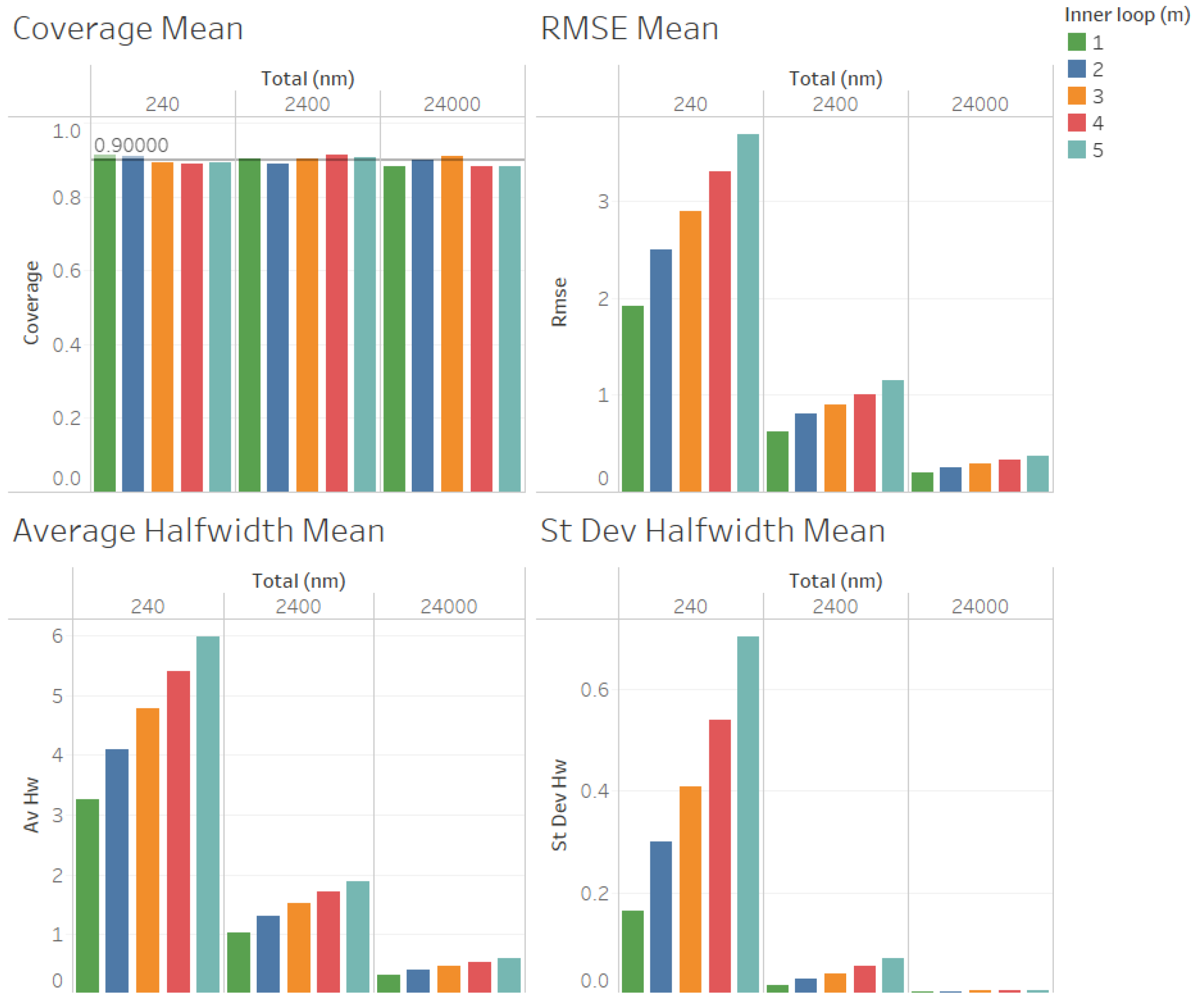
In Figure 3, we illustrate the performance measures for the quality of the estimation procedure that we obtained for the estimation of the point forecast $\alpha$ when $T=15$. As we can observe in Figure 3, the coverages are acceptable (very close to the nominal value of 0.9, even for $nm=240$). These results validate the ACI defined in (6) for the point forecast $\alpha$. We also observe in Figure 3 that the RMSE, average halfwidth, and standard deviation of the halfwidths improve (decrease) as the number of observations in the outer loop (n) increases, as suggested by Corollary 1. Note also in Figure 3 that a smaller value of m provides smaller RMSEs, average halfwidths, and standard deviations of the halfwidths, thus validating our suggestion that m should be as small as possible to improve the accuracy in the estimation of $\alpha$. 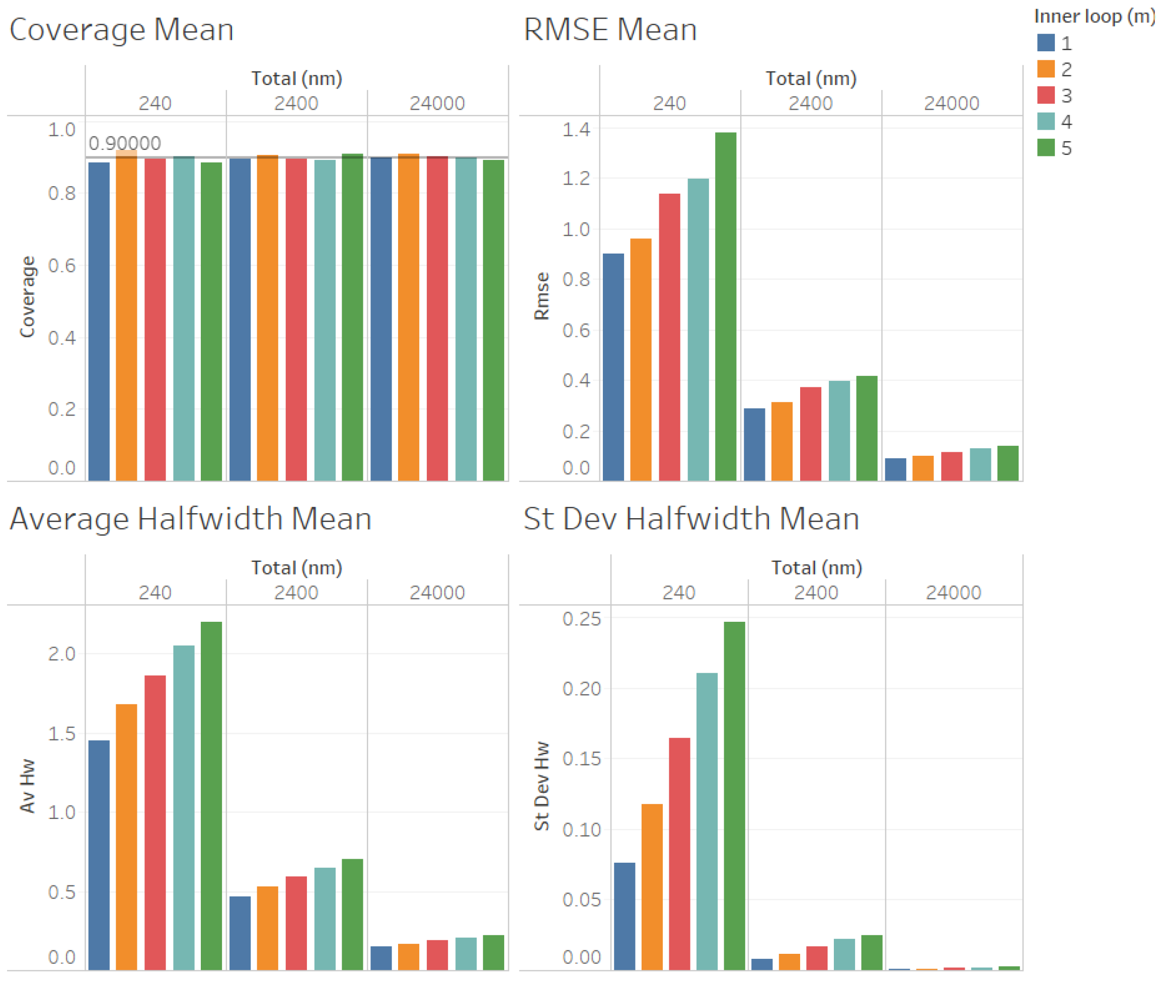In Figure 4, we illustrate the corresponding results for $T=5$, where we can observe that the same conclusions mentioned for $T=15$ are fulfilled, and the main difference from the previous case is that the RMSE, average halfwidths, and standard deviation of halfwidths are smaller, which is consistent with the fact that the point forecast $\alpha$ is smaller than in the case in which $T=15$. Note that both in the case of Figure 3 and in the case of Figure 4, the RMSE, average halfwidth, and average standard deviation of the halfwidths seem to be a linear function of m.

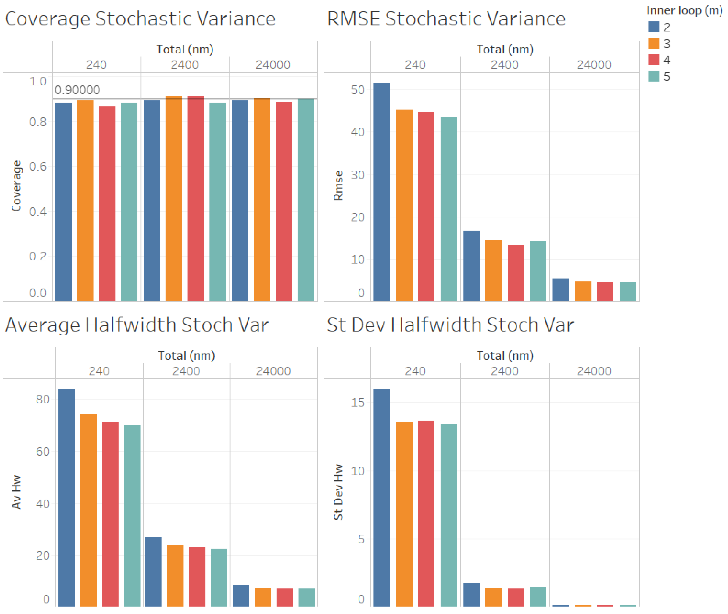
In Figure 5, we illustrate the performance measures for the quality of the estimation procedure that we obtained for the estimation of the stochastic variance ${\sigma }_S^2$ when $T=15$. As we can observe in Figure 5, the coverages are acceptable (very close to the nominal value of 0.9, even for $nm=240$). These results validate the ACI defined in (6) for the stochastic variance ${\sigma }_S^2$. We also observe in Figure 5 that the RMSE, average halfwidth, and standard deviation of halfwidths improve (decrease) as the number of observations in the outer level (n) increases, as suggested by Corollary 2. However, contrary to what we observed for the estimation of $\alpha$, a larger value of m provides smaller RMSE, average halfwidths, and standard deviations of the halfwidths, suggesting that, for a fixed value of $nm$, the quality of the estimation for the stochastic variance ${\sigma }_S^2$ improves as the number of the observations in the inner loop (m) increases, although the values are very close for $nm=2400,\mathrm{24,000}$. 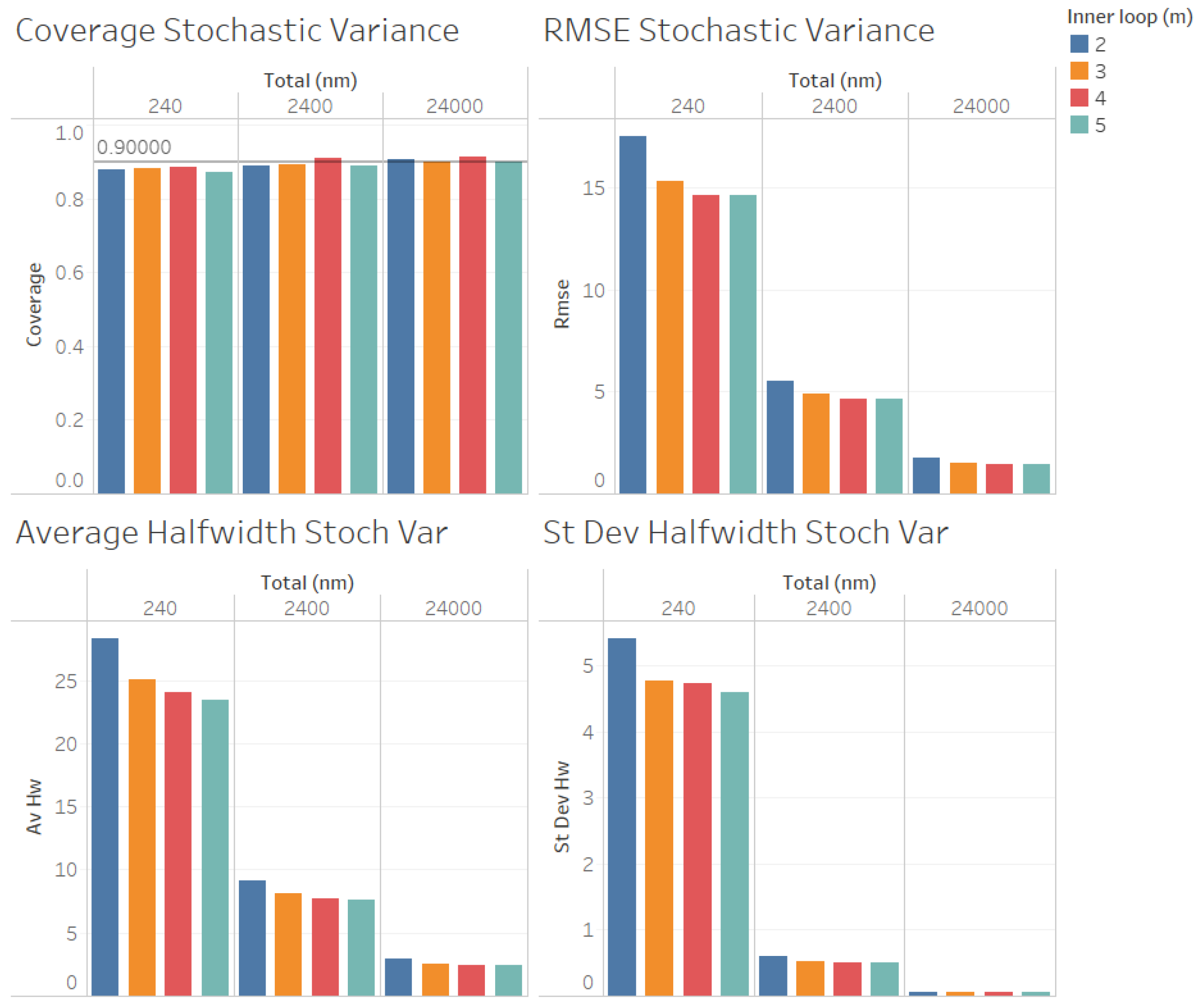In Figure 6, we illustrate the corresponding results for $T=5$, where we can observe that the same conclusions as those mentioned for $T=15$ are fulfilled, and the main difference from the previous instance that we observed is that, now, the RMSE, average halfwidths, and standard deviation of halfwidths are smaller, which is consistent with the fact that the point forecast $\alpha$ is smaller than in the case $T=15$. Contrary to what we observed for the case of the estimation of $\alpha$, note that both in the case of Figure 5 and in the case of Figure 6, the RMSE, average halfwidth, and average standard deviation of the halfwidth do not seem to be a linear function of m. We emphasize that the case in which $m=1$ is not considered in Figure 5 and Figure 6 because ${\sigma }_S^2$ cannot be estimated when $m=1$.

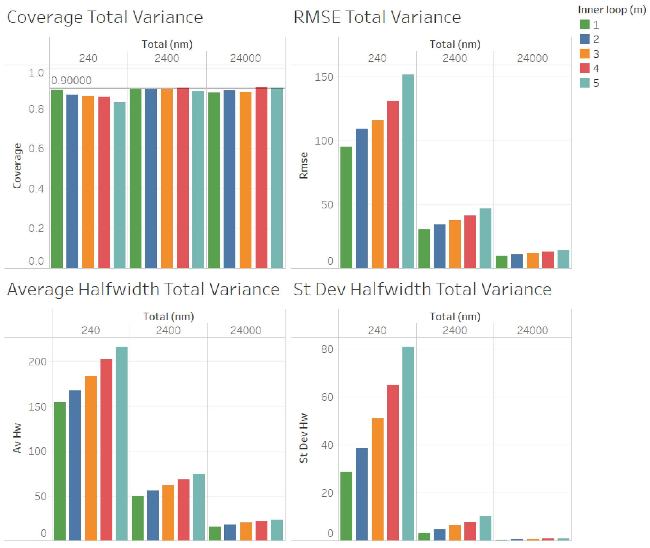
For the estimation of the total variance ${\sigma }_T^2$ (illustrated in Figure 7 for $T=15$, and in Figure 8 for $T=5$), we obtained results for the quality of the estimation that were similar to those for the estimation of the point forecast $\alpha$, except that larger values of n were required to obtain reliable coverages. As we can observe in Figure 7 and Figure 8, the coverages are acceptable (very close to the nominal value of 0.9, only for $n=2400$ and 24,000). These results validate the ACI defined in (6) for the total variance ${\sigma }_T^2$. We can also observe in Figure 7 and Figure 8 that the RMSE, average halfwidth, and standard deviation of the halfwidths improve (decrease) as the number of observations in the outer loop (n) increases, as suggested by Corollary 3. 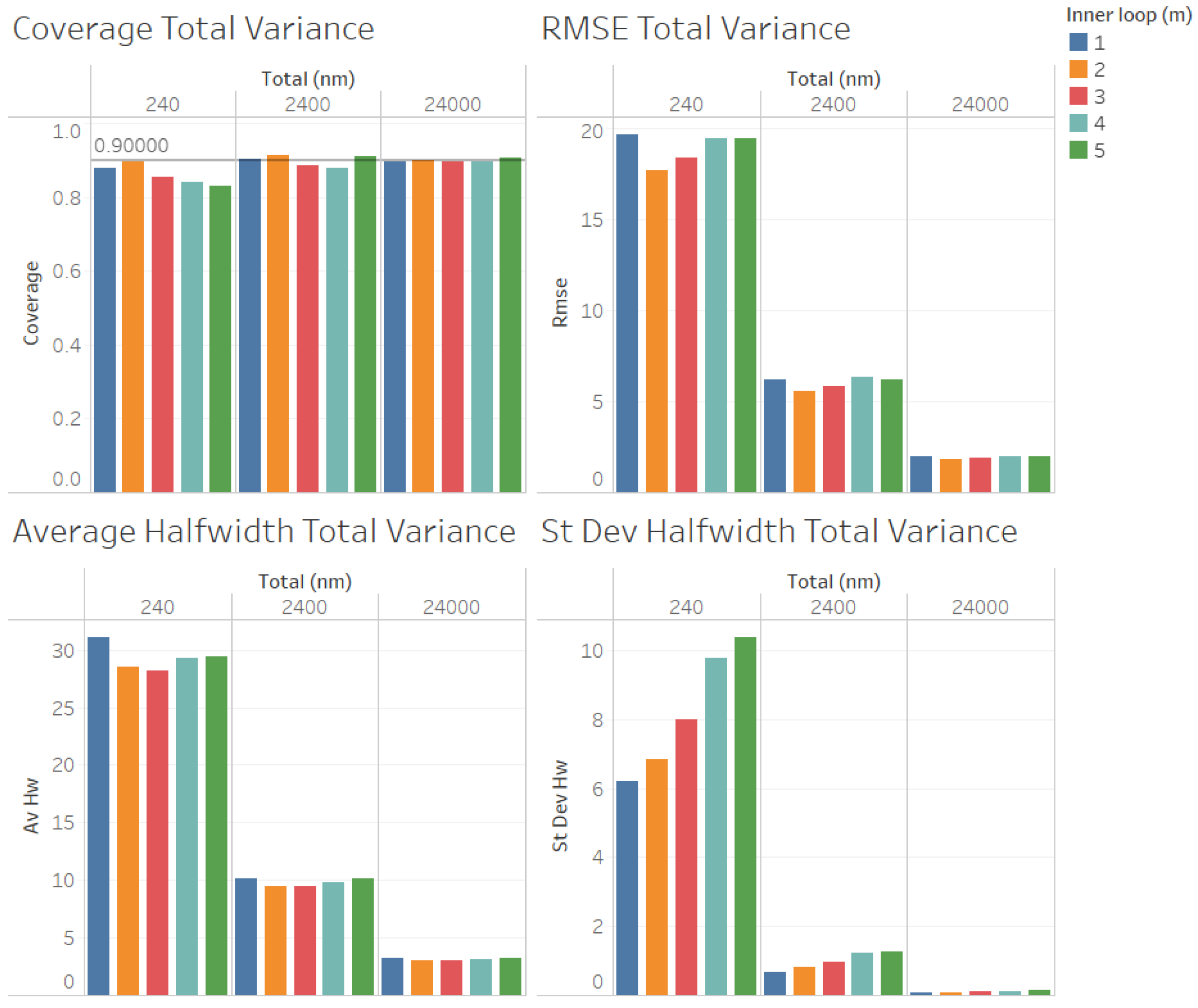Note also in Figure 7 that a smaller value of m provides smaller RMSEs, average halfwidths, and standard deviations of halfwidths. However, for the case in which $T=5$ (illustrated in Figure 8), where ${\sigma }_S^2>{\sigma }_P^2$, we observe that the RMSE and the average halfwidth decrease from $m=1$ to $m=2$ and then increase, showing that the best value of m for the estimation of ${\sigma }_T^2$ depends on the value of the ratio of ${\sigma }_S^2/{\sigma }_P^2$.

In a second set of experiments, we considered $nm=100,1000,\mathrm{10,000}$, with $m=1$, $m\approx {\left(nm\right)}^{1/3}$, and $m\approx {\left(nm\right)}^{1/2}$ for each value of $nm$, to compare the quality of the estimation procedures by using the value of m that we suggested as appropriate for the estimation of the point forecast $\alpha$ with other choices of p to illustrate the validity of Proposition 3.

Note that $m\approx {\left(nm\right)}^{1/3}$ is equivalent to $p=2/3$ in Proposition 3, and $m\approx {\left(nm\right)}^{1/2}$ corresponds to $p=1/2$. Note also that $m\approx {\left(nm\right)}^{1/3}$ corresponds to the value of m suggested in [5], which is a good option for the case of biased estimation in the inner loop of the algorithm in Figure 2. The results of this set of experiments are summarized in Figure 9, Figure 10, Figure 11 and Figure 12. Note that we do not consider the estimation of the stochastic variance ${\sigma }_S^2$ in this set of experiments because $m\ge 2$ is required to construct an ACI for the stochastic variance ${\sigma }_S^2$. Note also that we consider $a=100$, $b=1000$, $c=\mathrm{10,000}$, $a^{1/3}\approx 5$, $c^{1/3}\approx 20$, and $c^{1/2}\approx 32$, and we use the same color (red) for $m=a^{1/3},b^{1/3}$, and $c^{1/3}$, as well as the same color (yellow) for $m=a^{1/2},b^{1/2},$ and $c^{1/b}$, to report our results in Figure 9, Figure 10, Figure 11 and Figure 12.

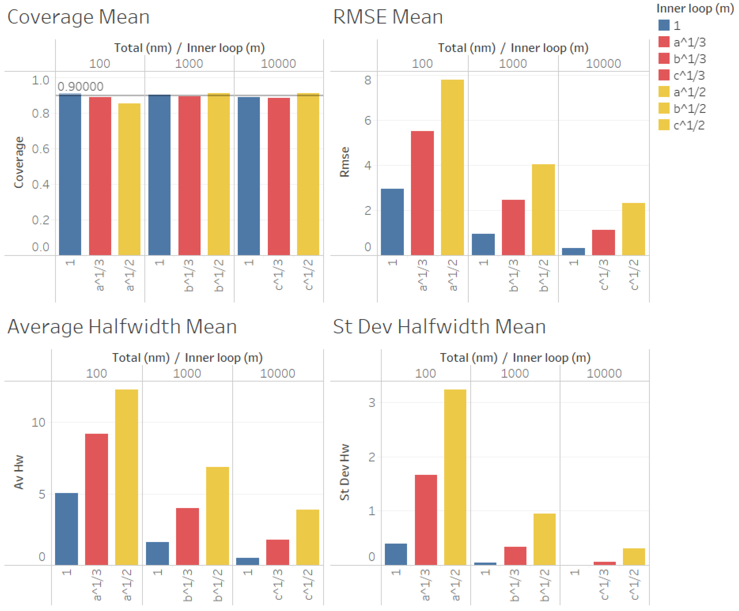
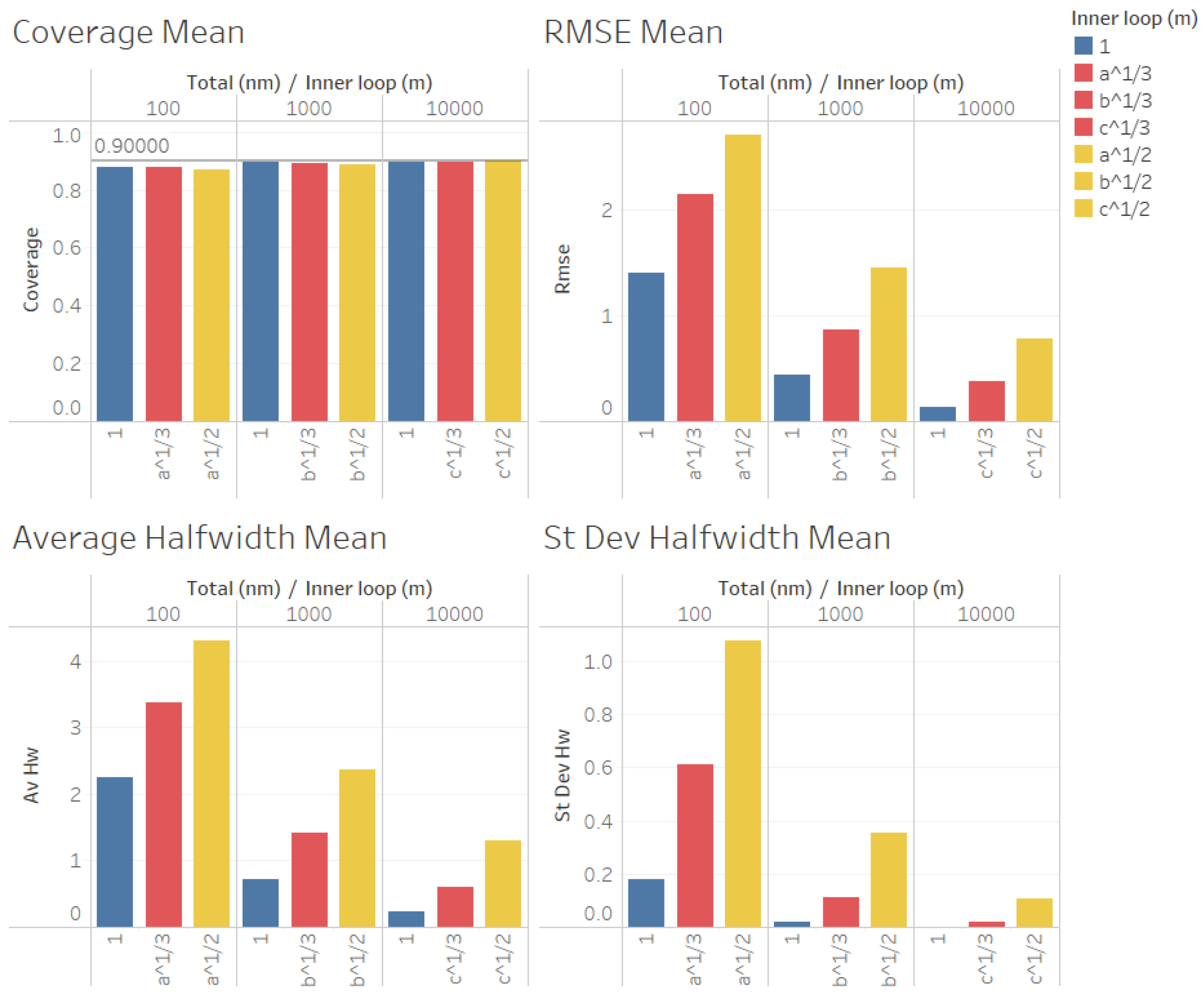
In Figure 9 and Figure 10, we illustrate the performance measures for the quality of the estimation procedure that we obtained for the estimation of the point forecast $\alpha$ in our second set of experiments. As we can observe in Figure 9 and Figure 10, the coverages are acceptable (very close to the nominal value of 0.9, even for $n=100$). These results validate the ACI defined in (6) for the point forecast $\alpha$ and the ACI suggested by Proposition 3. We can also observe in Figure 9 and Figure 10 that the RMSE, average halfwidth, and standard deviation of the halfwidths are worse than $m=1$ for $m\approx {\left(nm\right)}^{1/3}$, and they are even worse for $m\approx {\left(nm\right)}^{1/2}$, thus confirming our finding that, for a fixed number of simulated observations $k=nm$, a smaller value of m produces better point estimators for $\alpha$, confirming the result of Proposition 3.

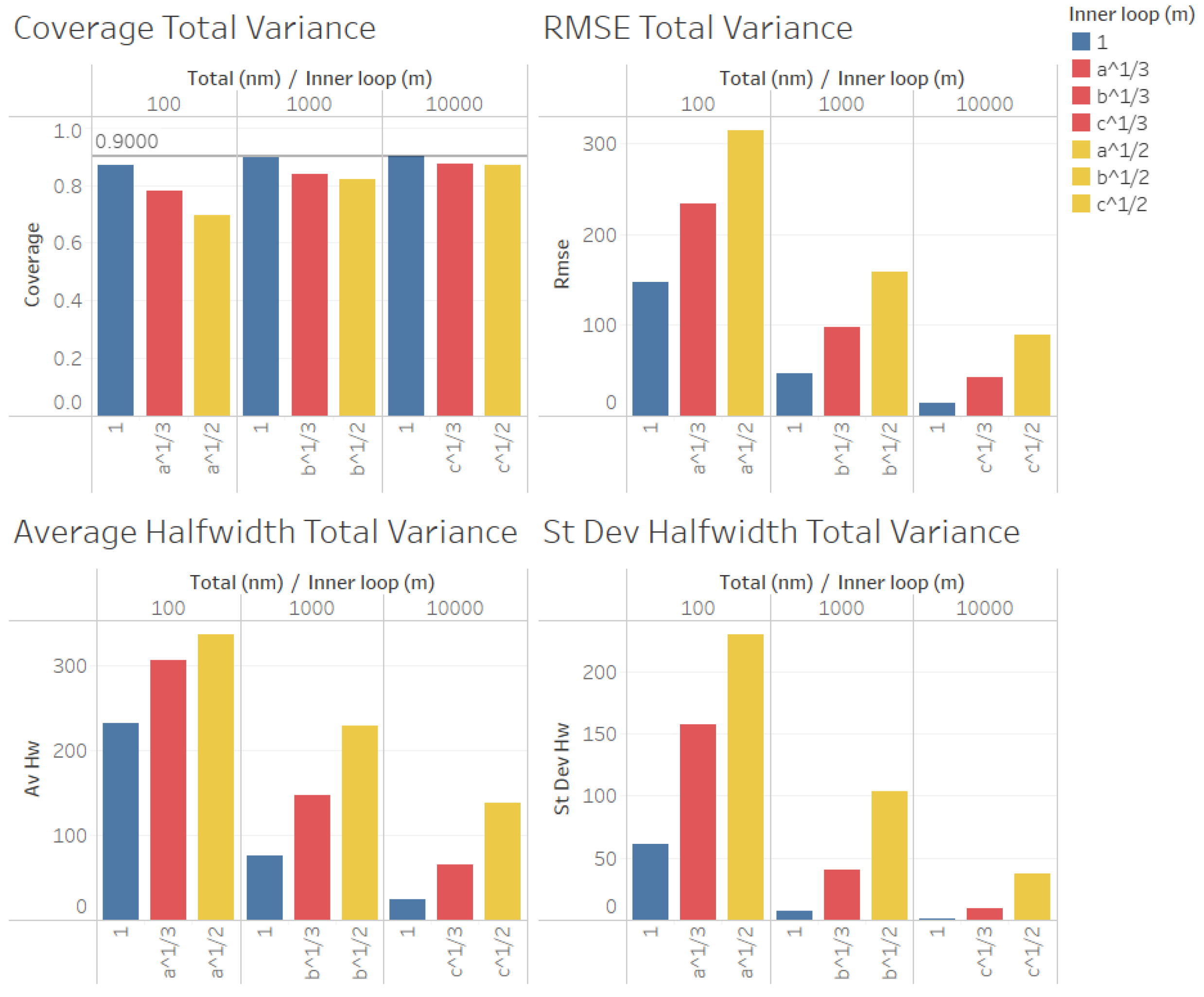
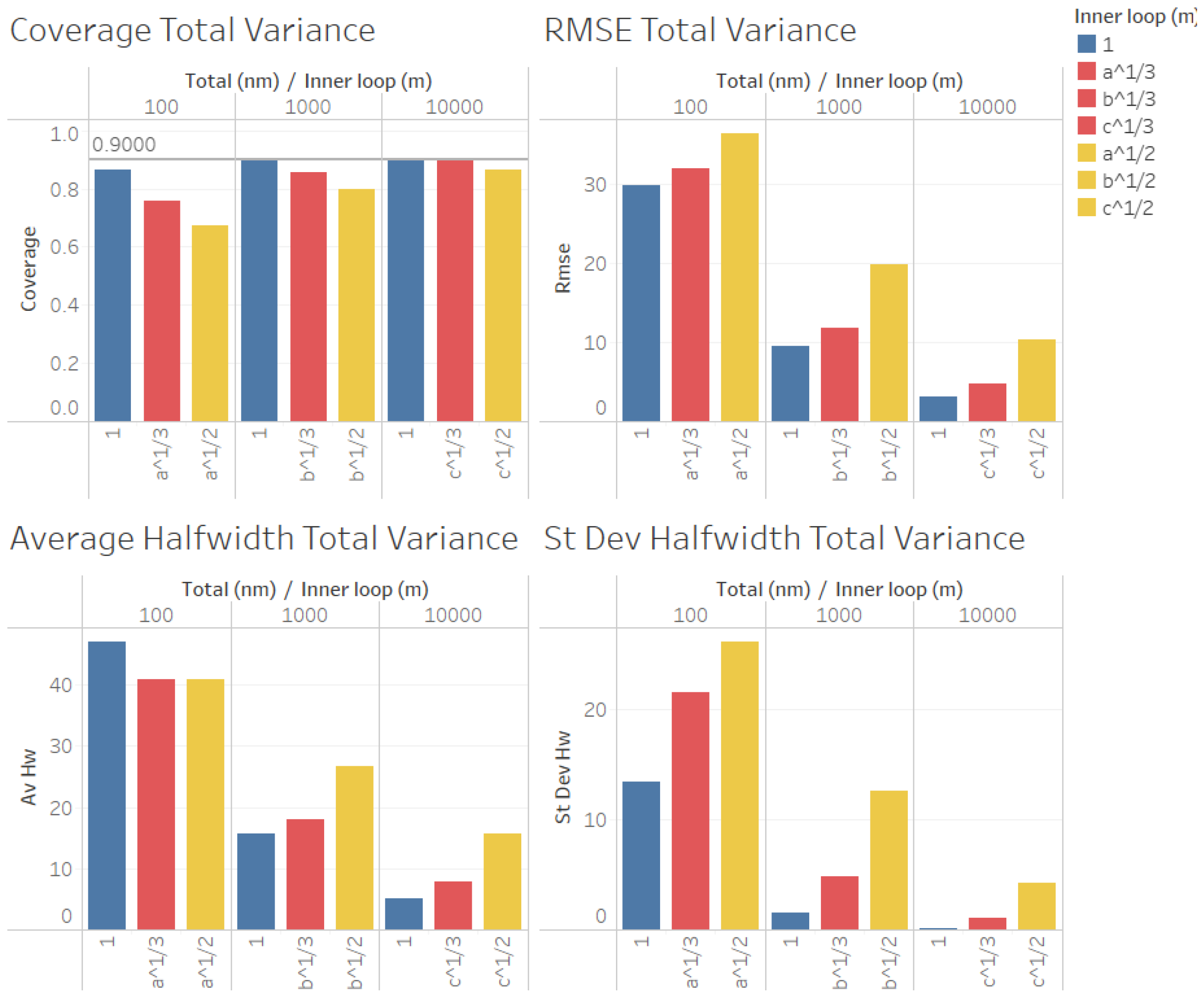
Finally, in Figure 11 and Figure 12, we show our results for the second set of experiments and the estimation of the total variance ${\sigma }_T^2$.

In Figure 11 and Figure 12, we found similar results to those for the case of the estimation of the point forecast $\alpha$, the coverages were very good (even for n = 100), and all measures of the quality of the point estimation (RMSE, average and standard deviation of halfwidths) were worse than those in the case in which $m=1$ for $m\approx {\left(nm\right)}^{1/3}$, and they were even worse for $m\approx {\left(nm\right)}^{1/2}$, suggesting that, as in the case of the estimation of $\alpha$, a smaller value of m produces better point estimators for ${\sigma }_T^2$ given a fixed number of replications $k=nm$, with the only exception in Figure 12 (${\sigma }_S^2>{\sigma }_P^2$) being for the case of the average halfwidths and $nm=100$, where the average halfwidth seems to decrease with the value of m.

5. Conclusions

In this article, we discussed methods for the estimation of both the point forecast and the variance components of Bayesian forecast models from the output of stochastic simulations by using a two-level nested algorithm in which the simulated observations at both levels of the algorithm are independent. Our main contribution is the development of valid asymptotic confidence intervals for assessing the accuracy of the simulation-based point estimators. These methods are particularly useful when there is uncertainty in the parameter values of the random input components of a forecast model, and we wish to incorporate this uncertainty into the simulation-based forecasting of the model’s performance measures.

The proposed point estimators and their corresponding halfwidths are asymptotically valid, as shown by the theoretical and experimental results, which show that the point estimators converge to the corresponding parameter values and that the halfwidths converge to the nominal coverage as the number of replications n of the outer level increases. In addition, the halfwidths corresponding to the proposed ACIs tend to zero (as $n\to \infty$), which normally occurs with the appropriate simulation-based estimators of performance measurements from the outputs of simulation experiments.

We also investigated the best option for the number of observations m in the inner loop of the algorithm given a fixed number of observations $k=nm$, and we found that the choice of only one observation ($m=1$) is the best option for obtaining the smallest variance of the point estimator for the expectation of a performance variable. However, for the estimation of the stochastic variance ${\sigma }_S^2$ in a two-level nested algorithm, $m\ge 2$ is required. On the other hand, for the estimation of the stochastic variance ${\sigma }_S^2$, our experimental results show that larger values of m are better, and the best choice of m depends on the ratio of ${\sigma }_S^2/{\sigma }_P^2$ for the case of the estimation of the total variance (${\sigma }_T^2$).

We remark that we did not consider the case of correlated observations in the outer loop of the two-level algorithm or the case of steady-state simulations, which may have important applications for simulation-based estimation by using Markov chain Monte Carlo (see [38]). In addition, experimentation with other computational procedures, such as quasi-Monte Carlo (see [6]) or Simpson integration, may be other directions for future research.