Simulation and Analysis of Line 1 of Mexico City’s Metrobus: Evaluating System Performance through Passenger Satisfaction

Abstract

The Mexico City Metrobus is one of the most popular forms of public transportation inside the city, and since its opening in 2005, it has become a vital piece of infrastructure for the city; this is why the optimal functioning of the system is of key importance to Mexico City, as it plays a crucial role in moving millions of passengers every day. This paper presents a model to simulate Line 1 of the Mexico City Metrobus, which can be adapted to simulate other bus rapid transit (BRT) systems. We give a detailed description of the model development so that the reader can replicate our model. We developed various response variables in order to evaluate the system’s performance, which focused on passenger satisfaction and measured the maximum occupancy that a passenger experiences inside the buses, as well as the time that he spends in the queues at the stations. The results of the experiments show that it is possible to increase passenger satisfaction by considering different combinations of routes while maintaining the same fuel consumption. It was shown that, by considering an appropriate combination of routes, the average passenger satisfaction could surpass the satisfaction levels obtained by a 10% increase in total fuel consumption.

1. Introduction

The Mexico City Metrobus is a BRT system that is part of the Mexico City (CDMX) integrated mobility network. It started operation in June 2005 with Line 1, and it currently has 7 lines, 283 stations, and runs 175 km of confined lanes. The metrobus plays a crucial role in the daily life of millions of residents of Mexico City, with Line 1 alone transporting 109,113,852 passengers between January and November 2022. This makes Line 1 of the Metrobus even more popular than 7 of the 12 lines of the Mexico City’s Metro [1].

The objective of the metrobus is to combine the efficiency and speed of a system such as the metro with the flexibility and low costs of a passenger bus system. As [2] mentions, a well-implemented and well-planned BRT system can provide a quality service that is comparable to that of a system with fixed tracks while also giving flexibility and much faster implementation times. Furthermore, as shown in [3,4], the CDMX Metrobus system has had a positive impact in the short term when it comes to reducing greenhouse gases in the city, and it represents a solution to improve the air quality in the city while also improving the mobility of the people within the city.

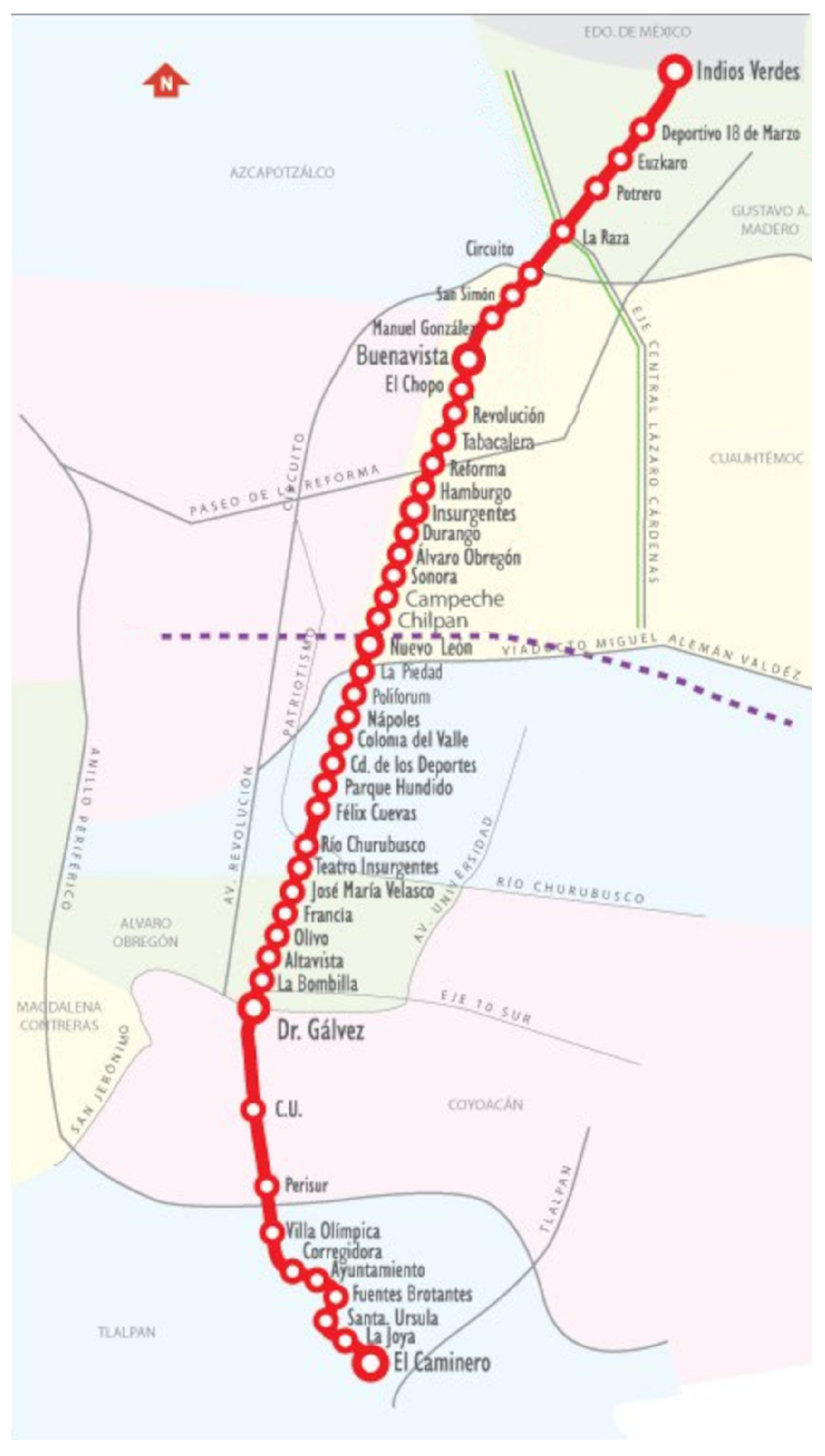
In this study, we focus on Metrobus Line 1, which runs along Av. de los Insurgentes, from edge to edge of the city, in the north and south directions. It has 46 stations in 28.8 km of road; see Figure 1. In addition, it has four routes that run exclusively on Line 1, three routes on Line 2 that join at Line 1, and one route on Line 3 that joins Line 3. Also, two types of buses pass through Line 1—articulate buses with a capacity of 160 passengers and biarticulated buses with a capacity of 240 passengers.

Our goal was to assess the current state of the Metrobus Line 1 while considering the control and response variables that we defined. Our control variables included the total number of buses on each route that are released to the system at every hour of the day. To measure the performance of the system, our response variables were defined as a function of passenger satisfaction. This is because, as mentioned by several authors (e.g., [5,6]), we consider that the passenger point of view is more important for determining the efficiency of public transport systems, since passengers are the ones using the system on a daily basis. However, we also have to consider objective measures, especially the operational cost, since this is a very big factor in determining what can be accomplished in the real world. As mentioned by [7], many of the BRT systems in the world are at a break-even point or are able to operate thanks to government subsidies (such as the Mexico City Metrobus); this is why it is important to improve passenger satisfaction without increasing operational costs. Once we have accomplished this, we propose experiments in order to understand how the response variables react to changes in the control variables.

To carry out our model, we used data provided by Metrobus through the National Transparency Portal (NTP), such as the number of arrivals at each station, the number of buses in the system, and the route times between stations, among others, for 2022.

As noted by several authors (see, e.g., [8,9,10]), scheduling in a stochastic environment is a difficult problem that can be approached by stochastic simulation; for this, we used the Simio package, which allows us to model all the necessary elements for this system [11].

In recent years, many investigations have been conducted to improve the performance and passengers satisfaction in public transport systems, particularly for BRT systems, using simulation. Below, we present a brief description of the various approaches that have been used to address this topic in order to situate this research in the context of the developments in this subject.

Gunawan [12] developed a framework to simulate BRT systems using discrete event simulation. Subsequently, a model was presented in which two stations and one pool of buses were considered, which could accurately reproduce the phenomena observed commonly in BTR systems. Campos et al. [13] proposed a discrete event simulation model of TransMilenio, the BRT system in Bogota, Colombia. To simulate the destinations of passengers, they used a user mix matrix, which represents the probabilities that a passenger originating at station i travels to station j, which they obtained through a survey of 660 passengers. In our model, the user mix matrix U was obtained through simulation, and we used a Bayesian approach, described in [14], at the start of each simulation run (see Section 3.3).

Other areas in which a simulation-based approach is commonly used to optimize BRT systems include in the implementation of traffic signal priority [15] and in the operation of bus stops [16]. Toledo et al. [15] presented mesoscopic traffic simulation and a genetic algorithm to perform the optimization. The research presented two case studies—transit priority at an intersection and a coordinated intersection. It was shown that there is potential for reducing passengers traveling times, but it also mentioned that the results obtained are not easily generalized. Lin et al. [16] proposed a combinatorial solution to reduce bus queues in the BRT system in Guangzhou, China by implementing multiple substops at each of the stations. It was shown that, by using this method, bus queuing could reduced, which has an impact on passengers’ traveling times and system saturation.

Other approaches have been proposed to optimize bus schedules. For example, Sharma et al. [17] proposed a multi-agent framework to plan the schedules of one-way routes in Malta, and it was shown that this has a better performance compared to the traditional approach using mixed integer linear programming. Another approach was proposed by Xue et al. [18] in which they used uncertainty theory and a bilevel programming model to optimize the frequency and time between departures of the 207 bus routes of Nanchang city, China; they demonstrated that this is an effective approach for reducing passengers’ travel times, but it has some limitations. Wang et al. [19] proposed a mixed integer nonlinear programming model in which they sought to optimize bus schedules and traffic signaling. To analyze the model, they considered the Fengpu BTR line in Shanghai, China and showed that the passengers’ traveling times could be decreased compared to a more traditional approach.

The aspect we highlight the most about this research is the development of a model in which it almost exclusively considers real operational data from the Metrobus as its input parameters. Using this approach, we developed a model which is capable of replicating the real-world system very accurately. Another important point to highlight is that, when we do not have enough data to accurately replicate the system, we used a posterior sampling algorithm (see Appendix B) in which we used a Bayesian approach to consider the uncertainty in the parameters appropriately. We aim for this study to be a helpful tool for evaluating new scenarios before their implementation in BRT or other public transport systems, as well as for future research about schedule optimization in a stochastic environment.

The remainder of this paper is structured as follows. First, in Section 2, we state the methodology for carrying out this investigation, and we also discuss the advantages and disadvantages of the method we propose. Then, in Section 3, we show the analysis made for the input parameter of the model and provide a justification for the assumptions made in the model. Afterward, in Section 4, we present the details for developing the model we produce; we try to be as clear as possible so that the reader can replicate our model. Next, in Section 5, we first state the control and response variables that our model considers; then, we define the three experiments that we conducted. Then, in Section 6, we show the results obtained from the three experiments and discuss them. Finally, in Section 7, we present our conclusions and provide directions for future research.

2. Research Methodology

In this section, we will present the methodology we followed to carry out this research. First, we will quickly discuss why we approached this problem using simulation. Subsequently, we will follow up with an overview of the steps that we are going to follow throughout this investigation and the reasons why we consider it appropriate to follow these steps. Following this, we will give an explanation of how we obtained all the data that we used in our model, as well as the methods that we used to process it. Finally, we will explain the software we used to make our model, thereby addressing the reasons why we considered using the Simio simulation software version 15.249.31576 (64-bit).

To start, let us discuss the reasons why simulation serves as the appropriate approach in our research. The main problem we face when using simulation is the uncertainty in the results, which makes the conclusions less precise. However, it provides us with the opportunity to obtain results for highly intricate systems that would otherwise necessitate multiple simplifications in an analytical model, thereby potentially compromising its validity. As noted in [10], scheduling in a stochastic environment is a very complex problem, since we have to consider several random factors; in the case of our model, the factors include the arrival of passengers at each of the stations, the transfer times between any two stations, etc. Using simulation will allow us to more accurately simulate the behavior of passengers and buses within the Metrobus Line 1; because of this, we will be able to obtain results that are more useful in the real world, as well as compare to the results that we would obtain from an analytical model with several simplifications.

To carry out this investigation, we are going to follow the steps suggested by various authors (e.g., [11,20]) to carry out a study using stochastic simulation. These include the following: input analysis, model development, experiment design, and output analysis. In the input analysis, we will analyze the variables that are pertinent to our model; in addition, we will present the methods used to find these values using real data. Later, we have to develop a model and check that it adheres as much as possible to Line 1 of the Metrobus. We will also have to verify and validate that the proposed model closely simulates the reality and that there are no errors that could compromise the results. In the experiment design, we have to define the control and response variables of the model that we want to analyze; in addition, we must define the scenarios in which we will analyze its performance. Finally, in the output analysis, we have to evaluate the results obtained in the experiments and make sure that we can draw valid conclusions.

In order to have a model that simulates Line 1 as closely as possible, we used real metrobus operational data, which was provided through the NTP. Additionally, to simulate the destinations of passengers, we used data from the National Institute of Statistics and Geography (INEGI), which tell us the origins and destinations of CDMX residents. All the data that we used regarding metrobus operations are from 2022, and data about passenger routes in CDMX are from 2017. The three main databases that we used are the bus compliance schemes, the entrance of passengers to each of the stations, and the origin destination survey in households in the metropolitan area of the valley of Mexico [21]. In order to process all the data, we used MATLAB, since, due to the large volume of data we have, it facilitated the manipulation of this data. All details on the input analysis are given in Section 3.

To develop our model, we used Simio, which is a stochastic simulation modeling software, which facilitated the development of the model, since the standard library of objects already contains all the elements needed for our model (see [11] for detailed descriptions of the Simio standard library). In addition, all these objects already have a basic logic built into them, which is very easy to adapt to our specific requirements. In our model, we primarily used the model entity and vehicle objects, which we used to represent passengers and buses, respectively. Furthermore, Simio is capable of creating 2D and 3D animations that reflect the behaviors of passengers and buses within our model; this proved to be very useful when verifying our model [22]. Additionally, Simio allowed us to analyze the results of our experiments very easily, since they facilitates the creation of descriptive statistics of the results from the experiments and the creation of graphs regarding these results, all of which proved very useful for performing the output analysis.

The most significant drawback we encountered while using Simio is the long-running times. This was primarily attributed to Simio’s ability to incorporate an extensive level of detail in the model, which significantly impacts the computational performance during simulation execution. In addition, another drawback worth noting is that Simio places emphasis on the animation of the model, which can also contribute to increase running times. Since animation is a useful tool for verifying the model, we have to pay close attention so that running times do not become very slow. Taking this into account, we decided that Simio was the right tool to develop our model, but we had to consider that the running times would be longer than if we used other software options. More details about the Simio simulation software can be found in [11].

3. Input Analysis

In this section, we describe how the available data was used to define the main random components of our stochastic simulation. We provide information on how the data was obtained, how it was manipulated, and how we finally implemented the data in our model. The vast majority of the data was provided by Metrobus through the NTP and also through the INEGI.

3.1. System Arrival Processes

To simulate the arrival process at each station, we assume that the arrival process at station i is a nonhomogeneous Poisson process (NPP) of $\{X_i\left(t\right):t\ge 0\}$ with an intensity rate function ${\lambda }_i\left(t\right)$ [23] so that the number of arrivals up to time t follows a Poisson distribution with the following expectation:

$${\Lambda }_i\left(t\right)={\int }_0^t{\lambda }_i\left(t\right)dt.$$

(1)

This assumption has been shown to be a reasonable approach for modeling customer arrivals (see, e.g., [24]). Furthermore, we assume that ${\lambda }_i\left(t\right)$ is a piecewise constant function that changes at every hour of the day, and we let ${\lambda }_{ij}$ be the intensity rate at station i from hour j to hour $j+1$ ($j=0,\dots ,23$). This asumption has been shown to be an effective way to model the arrival of customers when service demand throughout the day is not constant. For example, in [25], a piecewise constant function was shown to be an effective way to model the arrival of unscheduled patients throughout the day.

To estimate the intensity rate ${\lambda }_{ij}$ of the NPP at station i from hour j to hour $j+1$, we utilize the information of the number of arrivals observed at station i from hour j to hour $j+1$ for m so that we denote $m_{ijk}$ as the corresponding number of arrivals for day k ($k=1,\dots ,m$). If we let $x_{ijkl}$ be the interarrival time (in hours) between passenger $l-1$ and passenger l at the station i on the interval from hour j to hour $j+1$ and day k (we assume the arrival time of passenger 0 is j justified by the memoryless property of the exponential distribution), then they are independent and identically distributed (iid) as exponential with a rate of ${\lambda }_{ij}$ so that, for fixed k, the likelihood function becomes the following:

$$L_k\left({\lambda }_{ij}\right)=\left[\prod _{l=1}^{n_{ijk}}{\lambda }_{ij}{e}^{-{\lambda }_{ij}{x}_{ijkl}}\right]\left[e^{-{\lambda }_{ij}(1-{\sum }_{l=1}^{n_{ijk}}{x}_{ijkl})}\right]={\lambda }_{ij}^{n_{ijk}}{e}^{-{\lambda }_{ij}},$$

which means that the logarithm of the likelihood considering all data is given by

$$LnL\left({\lambda }_{ij}\right)=\sum _{k=1}^{m}ln\left(L_k\left({\lambda }_{ij}\right)\right)=\sum _{k=1}^m{n}_{ijk}ln\left({\lambda }_{ij}\right)-m{\lambda }_{ij},$$

(2)

and by equating the derivative (with respect to ${\lambda }_{ij}$) of this function to zero, we obtain the maximum likelihood estimator for ${\lambda }_{ij}$:

$${\widehat{\lambda }}_{ij}=\frac{{\sum }_{k=1}^m{m}_{ijk}}{m}.$$

(3)

Therefore, we use the arithmetic mean of the number of arrivals to estimate the values of each ${\lambda }_{i_j}$. For this process, we consider the average number of arrivals per station and per hour of the day during 2022. To obtain these estimates, we used data provided by Metrobus through the NTP, which contains the number of arrivals at each station of 7 lines broken down by date and hour. Also, to simplify the notation, we use ${\lambda }_{i_j}$ in place of ${\widehat{\lambda }}_{ij}$.

To simulate the number of arrivals at stations 47 and 48, corresponding to the auxiliary stations for Lines 2 and 3, respectively (details about this can be found in Section 4.4 and

Table A1. Station numbers in the model and station names of the Metrobus Line 1 and auxiliary stations.

Station ID	Station Name	Station ID	Station Name
1	Indios Verdes	25	Colonia del Valle
2	Deportivo 18 de marzo	26	Ciudad de los deportes
3	Euzkaro	27	Parque Hundido
4	Potrero	28	Félix Cuevas
5	La Raza	29	Rio Churubusco
6	Circuito	30	Teatro Insurgentes
7	San Simón	31	José María Velasco
8	Manuel González	32	Francia
9	Buenavista	33	Olivo
10	El Chopo	34	Altavista
11	Revolución	35	La Bombilla
12	Plaza de la República	36	Doctor Gálvez
13	Reforma	37	C.U.
14	Hamburgo	38	C.C.U.
15	Glorieta Insurgentes	39	Perisur
16	Durango	40	Villa Olímpica
17	Álvaro Obregón	41	Corregidora
18	Sonora	42	Ayuntamiento
19	Campeche	43	Fuentes Brotantes
20	Chilpancingo	44	Santa Úrsula
21	Nuevo León	45	La Joya
22	La Piedad	46	El Caminero
23	Polifórum	47	Line 2
24	Nápoles	48	Line 3

), we use ${\lambda }_{i_j}^{\prime }={\lambda }_{i_j}{c}_i$, where $c_{47}=\frac{317}{2272}$, and $c_{48}=\frac{216}{1272}$; for all other values of i, we simply consider the original ${\lambda }_{i_j}$.

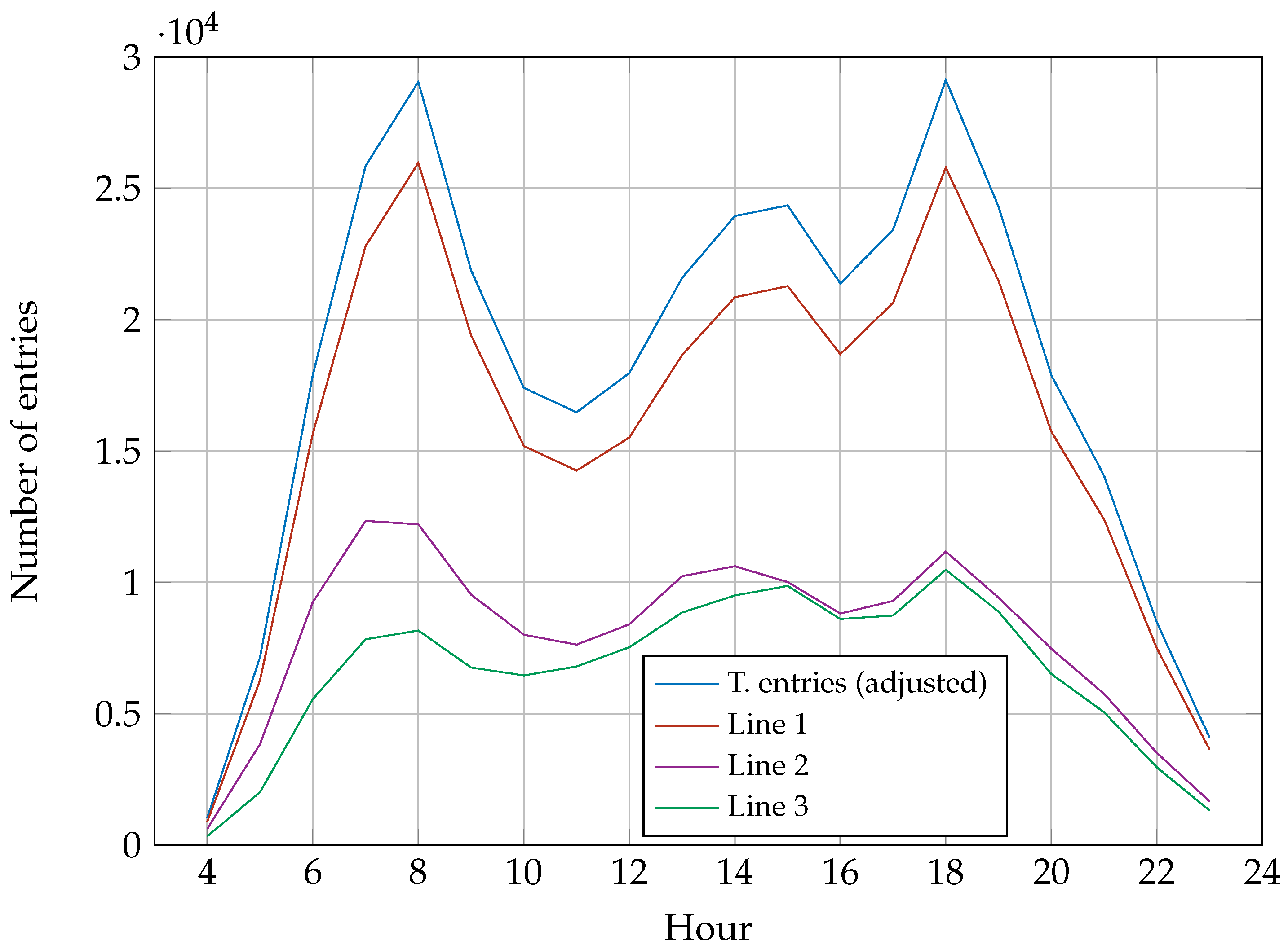
Here, ${\lambda }_{i_j}$ represents the average number of arrivals at all the stations of Lines 2 and 3 at time j, and $c_i$ is a constant that represents the proportion of passengers who travel from any of the stations on Lines 2 and 3 to any of the stations on Line 1. To calculate the value of c, we used data from [21], which provided us with the number of people who come from any of the stations that travel from Lines 2 and 3 to the stations on Line 1; more information about this survey is provided in Section 3.2. Figure 2 shows the total number of entries into the system on each of the lines and the total number of entries adjusted with the constant c.

It must be considered that, in this model, we are only simulating one day, regardless of the day of the week or if it is a holiday, which could have a significant impact on the rate of arrivals per station per hour; for this reason, we decided that, in order to simplify the model, we would only consider the average of all the days in the year 2022. The model can easily be adapted to simulate specific days of the week by adding a constant variable that accounts for the increase or decrease in passengers per day, as shown in a study provided by Metrobus [26]. However, in this model, we did not consider using the constant.

3.2. User Mix Matrix

As we will mention in Section 4.1.2, in this model, we assign the destination of the passengers based on a matrix $U\in {\mathbb{R}}^{48\times 48}$ in which its entries $u_{i,j}$ represent the probabilities that a passenger who originates at station j goes to station i; this matrix is simulated at the beginning of each simulation according to a Bayesian approach; see Section 3.3. In this section, we will discuss how we obtained our initial matrix A, which served as input for the simulation of the matrix U, and, in Section 3.3, we discuss the method we used to simulate the matrix U.

To obtain the input matrix for the initial simulation, we used data from [21]. The objective of this survey was to identify and record the routes that people traveled within Mexico City and the means of transportation they used. The survey considered various methods of transportation, both public and private.

To obtain the necessary data, we focused only on the question relevant to the metrobus. In the survey, the answers to the relevant questions for this model are the station of origin and the station of destination in the case where the transportation method was the metrobus.

We defined a matrix $A\in {\mathbb{R}}^{48\times 48}$ in which every entry $a_{i,j}$ represented the number of occurrences in the survey in which a passenger was going from station j to station i. For the cases in which the passenger was heading from or to a station in Lines 2 or 3, we recorded them all under auxiliary stations 47 and 48.

To simplify the model, we make the assumption all passengers that will perform a transfer from Lines 2 and 3 to Line 1 or vice versa, and they will do so inside one of the buses that follows a route that changes lines; this is based on the fact that, if we suppose that they walk as little as possible, the way to do this is to wait until the bus they are currently on arrives to a station in which the buses change lines. In addition, there are no incentives to transfer to any other station, since the passenger would end up traveling through more stations in this way. In the same way, we make the assumption that no passenger who goes from Line 2 to Line 3, or vice versa, will take this route within Line 1, since it is always faster to make the transfer from Line 2 to Line 3 directly than using Line 1 to connect them. Finally, we assume that no passenger will enter and leave the system at the same station.

3.3. Matrix Simulation

As we just mentioned in Section 3.2, the matrix we used to define the user’s destination, U, was simulated at the start of each run. The reason for this is that the matrix that we obtained from [21] only had 3600 observations, and the matrix has $48\times 48=2304$ entries, so we considered that there existed uncertainty due to several entries not being accurately represented, especially for entries that are equal to zero. In addition, this matrix played a key role when performing the experimentation, so we considered it appropriate to simulate this matrix at the beginning of each simulation.

To carry out the simulation, we followed a similar method as the one proposed in [14] (more details are provided in Appendix B), so we only simulated the matrix once at the beginning of each simulation run. For the simulation, we assume that the destination of a passenger follows a multinomial distribution, and the parameters are given by the simulation we are describing. Given this, we are going to consider as the parameter for our posterior distribution the column vector $a_j$ plus the vector $\left(\begin{array}{ccccccc}0.5,& 0.5,& \dots & 0,& \dots & 0.5,& 0.5\end{array}\right)$, which is a vector in which all of its entries are 0.5, except for entry j, which is 0. Since we suppose that the destination of a passenger based on his origin follows a multinomial distribution with probabilities in the column vectors of U, we simulates the matrix U using the Dirichlet distribution, which is Jeffrey’s (objective) prior for the multinomial distribution [27], with the parameter we just mentioned.

Since Simio does not have an algorithm for generating the Dirichlet distribution, we generated this from a gamma random variate generator. For this process, let $Y_1,\dots ,Y_{k+1}$ be independent gamma random variables with parameters ${\alpha }_i>0$ and $\beta =1$. Then, if we consider the following:

$$Y=\sum _{i=1}^{k+1}{Y}_i,$$

(4)

and

$$X_i=\frac{Y_1}{Y}.$$

(5)

Then $(X_1,\dots ,X_k)$∼$\mathrm{Dirichlet}({\alpha }_1,\dots ,{\alpha }_{k+1})$. The proof that this algorithm generates a random sample of the Dirichlet distribution using a gamma random sample is shown in [28].

We implemented this algorithm as a Simio process, which was executed at the beginning of each simulation. The algorithm takes as input the matrix A plus a matrix in which all its entries are 0.5, except the diagonal, which is 0, and returns the matrix U that we used for the simulation run.

3.4. Travel Times between Stations

To simulate the time it takes for the buses to travel between stations, we used data extracted from the metrobus compliance schemes, which indicate the times at which each of the buses passes through each of the stations. With this information, we calculated the time interval between every two stations.

Our first approach to simulate the times between stations was to fit the data we had into a probability distribution, which is an effective way to capture the effects of traffic congestion and traffic signals [24]. Some of the most common distributions for modeling this are the normal distribution [24], the log-normal distribution [29], and the gamma distribution [30].

To perform the goodness-of-fit tests, we used the Kolmogorov–Smirnov statistic and the Cramer–von Mises statistic described in [31], and we used the software “SimpleAnalayzer” to conduct the tests (the details of “SimpleAnalayzer” can be seen in [32]). Our test showed that the best fits were obtained using the Weibull and gamma distributions, but the test statistics we obtained were considerably large, so it was difficult to draw a valid conclusion. We consider this to be because the sample sizes we were using are really large (around 50,000 observations), which we consider to be causing a type II error. To fix this, we used the data we had to create an empirical distribution, wherein the travel times between the stations were sampled from the original data.

3.5. Number of Buses

To obtain the number of buses that were released from each of the parking lots by hour, we again used the metrobus compliance schemes, wherein we counted the number of times a bus passed through the first station after the parking lot at each hour of the day. Using this information, we could ensure that all stations in the model remained interconnected, with each station accessible via at least one combination of routes throughout all hours of the day.

In addition, the compliance schemes also provided us with the buses’ IDs, with which we were able to know which types of buses passed at what hour of the day. Since we were only simulating one day, we simply considered the average number of buses that left the parking lots per hour. If we wanted to simulate a specific day of the week, in the same way as with the number of passengers per station, we could add a constant that adjusts the number of buses for specific days of the week, but that is outside the scope of this study.

It should be noted that, in order to simplify the model, we considered routes C3 and C4 to be the same. This is because, in our model, these two routes work exactly in the same way, since we are not modeling Line 2. To take this into account, we summed the number of buses by hour of the day and type of bus for each of the two routes together and considered this as the total number of buses of route C3.

4. Model Development

In this section, we present a description of the elements necessary for the simulation. As we mentioned in Section 2, the model was developed in Simio using the standard library. Our goal when designing the model was to make it as close to reality as possible, and we especially followed the logic that a passenger would follow within the system. Also, it should be noted that the Mexico City Metrobus system operates from 4:30 a.m. to 12:00 a.m., but buses carry passengers on their way to the parking lot; because of this, we ended our simulation at 1:00 a.m. In addition, we started the simulation at 4:00 a.m. so that the buses would have time to distribute themselves across the system.

To simplify the model and focus only on Line 1 of the Metrobus, we did not model Lines 2 and 3 of the system; instead, we used two auxiliary stations (stations 47 and 48), which represented Lines 2 and 3, respectively. Because of this, the source object located in stations 47 and 48 (the source object represents the entrance to the station, and it is responsible for creating the model entities) will establish all the passengers that originate in Lines 2 and 3 have a station from Line 1 as their destination. In the same way, passengers that start in stations from Line 1 and have as a destination a station from Line 2 or 3 will be assigned to station 47 or 48, respectively, as their destination.

Due to the size of Line 1 and the level of detail we incorporated in our model, the complexity of the developed model is considerable. To address this, we provided some measurements of structural and software complexity, as described in [33]. Regarding structural complexity, our model has 96 different queues, one for each direction of the 48 stations, 48 source and sink objects, and 554 transfer nodes. Then, the model has 767 connections, of which 98 are the connections between the stations that the buses use, 293 are connections that the passengers use inside each of the stations, 288 are connections that the buses use inside the stations, and 88 are connections inside the buses’ parking lots. In addition, throughout the simulation run, the model created around 360,000 passengers, and each one had eight variables. In terms of software complexity, we used a computer with an Intel ® Core™ i9-7940x CPU @ 3.10 GHz, 14 cores, 28 logical processors, and 32 GB of RAM. On average, each simulation run (21 h) took around 3 h to complete. This time was almost doubled by sampling the times between stations, as shown in Section 3.4, from a table instead of generating them from a probability distribution.

4.1. Passengers

The first step in creating our model is to define the passengers. These are the backbone of our model, since, based on their definition, we obtain the performance metrics of our model. To define the passengers, we used Simio’s model entity object. Passengers can only move within the stations on pre-established paths that take them to the necessary nodes; in addition, passengers can only move between two stations inside a bus.

First, passengers were created in each of the station’s source objects, and we assigned the following three variables to each one:

• Origin;
• Destination;
• Direction.

4.1.1. Origin

The origin variable is an integer variable that takes values between 1 and 48, thus indicating the station in which the passenger entered the system. A value between 1 and 46 indicates the station from Line 1 in which he was created, a value of 47 indicates that the passenger was created in the auxiliary station for Line 2, and a value of 48 indicates the auxiliary station for Line 3; check the Appendix A for details. Additionally, if the passenger makes a transfer to another bus, the value of the origin variable is updated to that of the station where the transfer is made.

4.1.2. Destination

In the same manner as the origin variable, destination is an integer variable that takes values between 1 and 48, which represent the final destination of each passenger (see Appendix A). This variable is also assigned at the time the passenger is created. To assign this variable, we used the “UserMix” matrix, which we represent by U, which we simulated at the beginning of each run using a Bayesian approach (we present more details as to how this matrix is simulated in Section 3.3). Each column $u_j$ represents a probability vector in which each element $u_{i,j}$ represents the probability that a passenger who originated at station j has station i as his destination (we present details in Section 3.2). Then, the destination variable takes the value of i using the probabilities from the vector $u_j$.

4.1.3. Direction

The direction variable is also an integer variable which can take a value of −1 or 1, which indicates the direction in which the passenger must travel to reach his destination. A value of −1 indicates that the passenger is traveling to the south, and a value of 1 indicates that the passenger is traveling north. To calculate this value, we use the following formula:

$$d=\left\{\begin{array}{cc}1& \mathrm{if}o-s>0\\ -1& \mathrm{if}o-s<0,\end{array}\right.$$

(6)

where d is the direction of the user, o is the origin, and s is the destination. If the passengers have stations 47 or 48 as their origin or destination, we use auxiliary values to calculate the direction of the users; if $o,s=47$ we use $o,s=20.5$, and if $o,s=48$ we use $o,s=9.5$. This is because the connection between Lines 1 and 2 occurs after station 21 in the north direction, and the connection between Lines 1 and 3 occurs after station 9 in the south direction. Finally, if a passenger transfers to another bus, we again calculate the value of the direction using the updated value of the origin variable.

Once these three variables are assigned, the passenger goes to the north or south platform, depending on the direction variable, to wait for a bus. Once the passenger arrives at the platform node, a process is started that counts the time the passenger spends in a queue waiting for the bus. This time only considers the time spent in each individual queue; it does not consider the time spent in other queues in case a passenger has to make multiple queues in the case of bus transfers.

Once the bus arrives at the station, two different processes occur. In the first one, which is executed before the passenger boards the bus, the passenger decides if the bus that just arrived at the station is moving in the same direction as the passenger’s travel path; this is based on the route that the bus follows. If this is the case, the passenger boards the bus and decides if the current bus will get him to his destination station. If the bus does not pass through the destination station, the passenger decides to make a transfer to another bus. If the bus that just arrived at the station is not going in the same direction as the passenger’s travel path, he will wait for the next bus to arrive at the station and trigger the same process again. This is done to prevent passengers from spending more time than necessary in the system. As noted in Section 3.5, eventually a bus that is going in the same direction as the passenger’s travel path will arrive at the station; this is because the total number of buses for each route at each hour of the simulation run ensures that all stations are connected by at least one combination of routes.

Once inside the bus, the second process is executed, wherein the passenger decides his decent station. In the event that the bus that the passenger is riding passes through the destination station of the passenger, the passenger will set his decent node as the platform of his destination station. If the passenger has to make a transfer, he will set his descent node as the platform of the station that is on the route of the bus that is closer to his destination station. This will almost always be the last station of the route, or in the case of passengers transferring from or towards Lines 2 or 3, they will set their descent nodes to the platform of stations 21 or 9, respectively, since these are the stations that bring them the closest to their destinations.

In the case where the passenger makes a transfer, once he gets off the bus, he will go back to the exit platform of the station where the transfer is made. While going to the platform, a process is executed in which the origin variable is updated to the number of stations in which the transfer is made; then, the direction variable is also updated using the new origin and the original destination to calculate it. Again, in the case where the origin or destination is station 47 or 48, we use the same auxiliary values as described in Section 4.1.3. Finally, a counter keeps track of the total number of transfers that a passenger has made, another counter keeps track of the total time spent in lines, and, lastly, we record the maximum occupancy that the bus, in which the passenger rides, reaches while the passenger is on board. All these steps are repeated until the passenger reaches his destination station.

Lastly, once the passenger reaches his destination, he heads to the exit of the station and reports the total time spent in queues, as well as the total number of transfers the passenger made to get here; all these values that the passengers reports are used to compute a satisfaction metric that we is use to evaluate different scenarios in our experiments; more details can be found in Section 5. Finally, the passenger is destroyed at the exit of the station, which is modeled with a sink object. Figure 3 shows the logic that we just describe, which every passenger in our model will follow.

4.2. Buses

As we have already mentioned in Section 1, there are a total of eight routes operating within Line 1—four are exclusive to Line 1, three lie between Lines 1 and 2, and one lies between Lines 1 and 3. The connection between Lines 1 and 2 occurs before station 21, and the connection between Lines 1 and 3 occurs after station 9. In addition, there are two types of buses: articulated—with a capacity of 160 passengers—and biarticulated—with a capacity of 240 passengers. Next, we present a table with the different routes that we are modeling and their characteristics.

To simulate the different routes and types of buses, we used the vehicle object from the Simio standard library. We defined a different vehicle for each of the routes and types of buses; in addition, because we have parking lots in the north and south terminals of each of the routes in the model, we also added a different type of bus so that their home nodes would be in the south parking lots. So, in total we have 22 different types of vehicles to represent each of the different types of routes, types of buses, and parking lots.

All buses follow a fixed sequence of nodes (route), which has to include all nodes through which a bus passes. Each type of vehicle needs its own route, because all of them enter a different pool when they arrive at the parking lots, and the north and south types of vehicle also need a different route, since they have different home nodes. For each type of vehicle we have in the model, we created 75 instances of them so that there would always be buses available at all the parking lots; this number did not affect the total operational cost, because those costs were calculated using the number of trucks that were circulating in the system (more details on how costs are calculated can be found in Section 5). All buses stop for 30 s at each of the stations on their routes; this is so that passengers can get on and off the buses. To simulate the time that a bus takes between two stations, we used time paths from the standard library; this made it easier to simulate the variations in time between the stations due to various factors. When a bus enters the time path, we simulate the time between both stations using an empirical probability distribution, as described in Section 3.4.

To model the number of buses in the system, we used real data on how many buses exited each of the parking lots at each hour of the day, see Section 3.5. Using that number, we set a timer so that the parking lot exit node released that number of buses uniformly throughout the hour. To release the buses, we created a process that first reads from a table the total number of buses that have to leave the parking lot at a certain hour; then, we calculated the time interval so that buses would be released at a uniform rate throughout the hour, and it releases the buses from the parking lot in that interval of time. It should be noted that the simulation starts running at 4:00 a.m., but the metrobuses start their operations at 4:30 a.m.; to fix this, we released twice the number of buses that we obtained from our data between 4:00 a.m. and 5:00 a.m. so that the buses would have time to distribute themselves across the system, and the real number of buses would be released from 4:30 a.m. and 5:00 a.m.

4.3. Parking Lots

Parking lots are located at the terminal stations of each of the routes; this can be found in

Table 1. Routes that operate within Line 1.

Routes *	Stations Traveled by Route	Lines in Which Operates	Type of Buses	Route Length in km (One Way)
A1	1–36	L1	Biarticulated	19.2
A2	1–15	L1	Biarticulated	9.6
A3	9–46	L1	Biarticulated	21.95
A7	1–46	L1	Biarticulated	28.8
A32	1–9 and 48	L1 and L3	Articulated and Biarticulated	16.35
C3	21–25 and 47	L1 and L2	Articulated and Biarticulated	18.1
C4	21–25 and 47	L1 and L2	Articulated and Biarticulated	14.1
C21	21–36 and 47	L1 and L2	Articulated	23.3

* These are the routes that we included in our model; there can be other routes that are not common for them to operate on a daily basis. Route C4 is not considered as an independent route in our model; rather, as part of route C3, more details are given in Section 3.5.

. Each parking lot serves as a pool of buses that is ready to dispatch according to the total number of buses that have to leave each the parking lots at each hour, depending on the route and type of bus. We explain how we calculated this number in Section 3.5.

In each parking lot, there is a different pool for each route and type of bus that is allowed to access that specific parking lot. At the entrance of each parking lot, there is a node that sends each bus to its corresponding pool. It should be noted that buses with the same route and capacity, but a different parking lot as their home node, are sent to the same pool. At the exit of each pool, there is a node that is responsible for releasing buses according to the total number of buses that depart each hour.

4.4. Stations

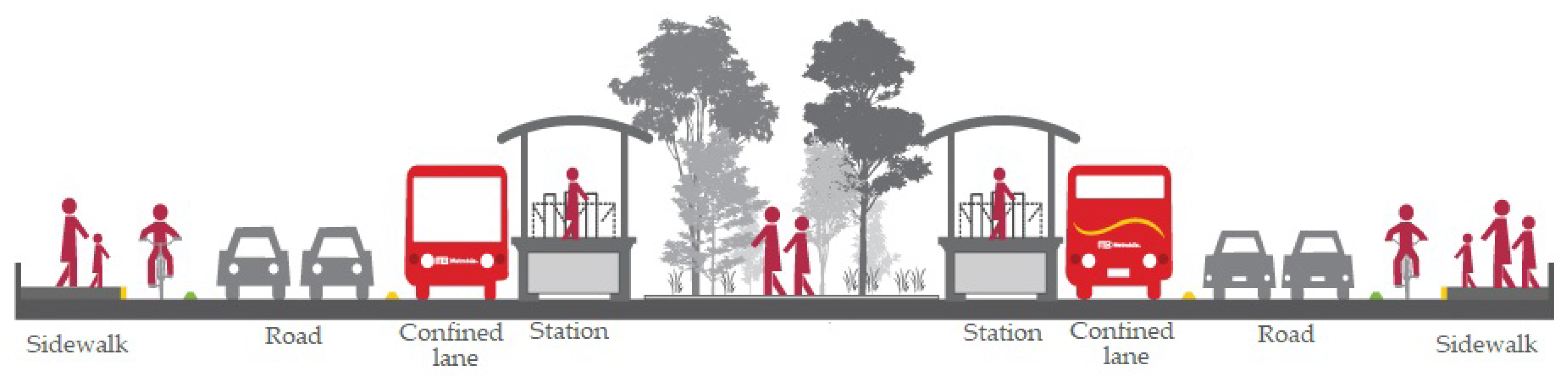
For each of the 46 stations in Line 1, as well as the auxiliary stations for Lines 2 and 3, we used the same station design. The objective of this was to facilitate the implementation of more or less stations so that it could be easily adapted to other systems. We designed the stations so that they resemble the actual stations in terms of the decisions that passengers have to make inside the stations to get onto the right buses and to be able to make transfers between the buses, Figure 4 shows the layout of each of the stations in Lines 1, 2 and 3. In the Mexico City Metrobus system, the stations are just elevated platforms where passengers wait for the buses, and transfers are done inside the elevated platform, because all the different routes that use one station use the same arrival and exit platforms.

To simulate the entrance of passengers to a station, we used the source object that creates passengers according to a nonhomogeneous Poisson process, as described in Section 3.1. Once inside the station, the passenger decides whether he wants to go to the north or south platform of the station according to the value of the direction variable. Then, he moves to the platform, gets in the queue, and waits for an appropriate bus according to the process we describe in Section 4.1. When the bus arrives at the station where the passenger wants to descend, the passenger drops off the bus at the arrival platform and walks to the center of the station. Then, he decides if this station is his final destination or if he has to make a transfer. In the case that this station is his destination, the passenger walks to the exit and it is destroyed by the sink object; in the case that the passenger is just making a transfer, he walks to the center of the station and again decides to which platform he has to go in order to arrive at his destination.

As we have already mentioned, all the stations are connected using time paths so that we can simulate the time between two stations. In the nodes where two time paths intersect, for example, when Lines 2 or 3 intersect Line 1, we have to indicate which path we want the buses to take to ensure that buses follow their specified route. In addition, we have to make sure to indicate that passengers cannot enter this time path unless they are riding a bus.

4.5. Verification and Validation

The last step in the development of the model is verification and validation. To perform this step, we used some of the techniques presented in [22]. For this, we considered the original number of buses that we obtained in Section 3.5, and the simulation was set to run between 4:00 a.m. and 1:00 a.m. on the following day.

First, we used animation to verify that the model behaved as we intended so that it mimicked the system as closely as possible. It should be noted that animations need to be carefully used, since it is easy to overlook problems that might arise in the long run. Since the simulated time of our experiments was set to 21 h, we checked through the full simulation that all the passengers only moved along the intended paths inside the stations and that they boarded a bus to get to any other station. We also checked that the buses only traveled along their corresponding routes and that the parking lots worked as intended, thus making sure that all buses arrived to their corresponding pool and were released according to the schedule they followed. By using animation, we concluded that our model worked as we wanted.

Another method we used to verify the model was to record the total number of passengers at each hour of the day. By doing this, we could ensure that the model was creating and destroying passengers as intended so that there would be no passengers stuck in any of the buses or stations.

In Figure 5, we can see that the average number of passengers inside the system at every hour of the simulation behaved very similarly to the total number of entries by hour of the simulation. This shows us that our model is capable of moving passengers from their starting stations to their destinations without having passengers stuck inside the buses or waiting at the stations.

The validation of or model and results was difficult, because we were unable to find quantitative data about passengers’ satisfaction, traveling times, or queue lengths at the stations; because of this, we cannot compare real data to the simulated data. Another approach we can use to validate our model is sensitivity analysis, with which we can determine if the behavior of the model is in accordance with what is expected. In Section 5.4, we present an experiment in which we varied the total number of buses by changing the total fuel consumption during the day. The result of this experiment, shown in Section 6.2, showed that the response variables we were recording, such as passenger satisfaction, queue lengths, etc. (more details are given in Section 5.2), reacted according to the changes in the total number of buses. In addition, Reference [22] mentions that animation is a good means to obtain the face validity of causal models. We consider our model to be causal, since the output of the model depends only on past and current inputs. Because of this, we validated the results obtained by our model using sensitivity analysis and animation.

5. Experiment Design

In this section, we present the details of the experiments we conducted and the variables we used. First, we give a description of the control variables that our model used. Afterwards, we give a description of the response variables that we defined, and, finally, we give a description of the experiments that we conducted so that the reader can reproduce our experiments.

5.1. Control Variables

As we have already mentioned, the control variables in our model are the number of buses that leave each of the parking lots by route and hour. It is important to note that, to simplify the model, we assume that the same number of buses, from each route, leave the north and south parking lots at each hour. In real life, this is not the case, but, by making this assumption, we reduced the total number of variables by half (which is very significant, since our model has 189 control variables).

5.2. Response Variables

Our model has six response variable, which are the following:

• Average satisfaction
• Average maximum bus occupancy;
• Average queue satisfaction;
• Total fuel consumption;
• Average bus occupancy;
• Average queue length.

In addition, we recorded all these values for each hour of the day.

5.2.1. Satisfaction, Maximum Bus Occupancy, and Queue Satisfaction

The level of passenger satisfaction is the primary response of the model, and with respect to this, we evaluated the performance of the different scenarios that we proposed. In this way, we tried to estimate the satisfaction of each of the passengers while taking into account the maximum occupancy that a bus reaches while the passenger is on it and the time spent in queues. To obtain these values, we assigned two variables to each of the passengers that recorded these values.

The maximum occupancy is a value between 0 and 1. To calculate this, the passenger checks the occupancy of the bus after it leaves each station, and if the value of bus occupancy is larger than the recorded maximum value of occupancy of the passenger, he updates it with the new value.

The value for queue satisfaction is obtained with the following function:

$$f\left(t\right)=\left\{\begin{array}{cc}1& t<3\\ 0.5& 3\le t<5\\ 0& 5\le t,\end{array}\right.$$

(7)

where t is the time spent in the queue in minutes.

With these two values, we can calculate the satisfaction as follows:

$$s=(1-o)+q,$$

(8)

where s is the satisfaction, o is the maximum bus occupancy, and q is the queue satisfaction. Because of this, the satisfaction level is a number between 0 and 2, which we sought to maximize during the experiments. The individual values of maximum occupancy and queue satisfaction were also reported as response variables.

5.2.2. Total Fuel Consumption

In order to calculate the total fuel consumption, we first have to estimate the number of liters consumed for each kilometer of travel. Using data from the official website of the Metrobus system [34], we can conclude that one full biarticulated bus consumes 1 L per kilometer traveled. Then, using data from the bus manufacturer’s website [35], we know that an articulated bus weights 30,000 kg, and the biarticulated model weighs 40,500 kg. Using this information, we assume that the fuel consumption of the articulated bus is 0.74 L per kilometer traveled.

To calculate the total fuel consumption for the day, we simply use the total number of buses on each route and type that will be released throughout the day. With these numbers, we can calculate the total distance traveled, check Table 1, by all buses, and multiply it by their corresponding fuel consumption per kilometer. The total fuel consumption is calculated at the beginning of each simulation run, since this value is completely deterministic.

5.2.3. Bus Occupancy

This value records the percentage of occupancy that each of the buses has after exiting each of the stations if they carry at least one passenger. Unlike the maximum occupancy value, this is reported at each of the stations and is not specific to any passengers or buses.

5.2.4. Queue Lengths

Aside from reporting the level of satisfaction of the passengers in the queue length, we also report the average length of the queues. This value is obtained by recording the entrance and exit times of each of the passengers onto the exit platforms nodes in the cases where the passenger gets in a queue (we do not consider the case in which the passenger queue time is equal to 0).

5.3. First Experiment

The goal of our first experiment was to find the values of the response variables using the current schedule that the metrobuses have. To achieve this, we used the number of buses that we obtained in Section 3.5 as the values of the control variables. In this experiment, we simulated between 4:00 a.m. and 1:00 a.m. of the next day (21 h) and ran the simulation 40 times in order to reduce the variability of the response variables.

To calculate the required number of replications, let us denote $w_i$ to be a simulation output of the ith independent replication, $i=1,\dots ,n$, let $\widehat{\mu }\left(n\right)$ be the sample mean, and let $\widehat{\sigma }\left(n\right)$ be the sample variance. By running the simulation experiment for $n=20$ and $n=40$ replications, for the satisfaction response variable, we obtained $\widehat{\mu }\left(20\right)=1.194$, $\widehat{\mu }\left(40\right)=1.195$, $\widehat{\sigma }\left(20\right)=0.00695$, and $\widehat{\sigma }\left(40\right)=0.0067$. We can compute the half-width for the asymptotic confidence intervals of $\mu$ using the following:

$$HW\left(n\right)=\frac{\widehat{\sigma }\left(n\right)}{\sqrt{n}}{t}_{(\frac{\alpha }{2},n-1)},$$

(9)

where $t_{(\frac{\alpha }{2},n-1)}$ is the Student’s t distribution with $n-1$ degrees of freedom [36]. If we consider $\alpha =0.01$, we obtain $HW\left(20\right)=0.0044$ and $HW\left(40\right)=0.0029$, which represent only 0.37% and 0.24% differences with respect to the sample means of 20 and 40 replications, respectively. Because of this, in the following experiments, we considered only 20 replications for each scenario.

5.4. Second Experiment

The objective of the second experiment was to understand the sensitivity of the response variables to changes in the total number of buses in the system. To achieve this, we added a constant variable that multiplies the total number of buses that leave the parking lots during the day. For this variable, we used values between 0.75 and 3. It is important to note that, in this experiment, we multiplied all control variables by the same number in each scenario so that the proportion of buses of each route and type would be the same as in the experiment described in Section 5.3.

In this experiment, we considered 24 scenarios in which we changed the value of the variable described above. We ran 20 replications for each scenario. In the same way as in Section 5.3, we simulated 21 h, which corresponds to one day.

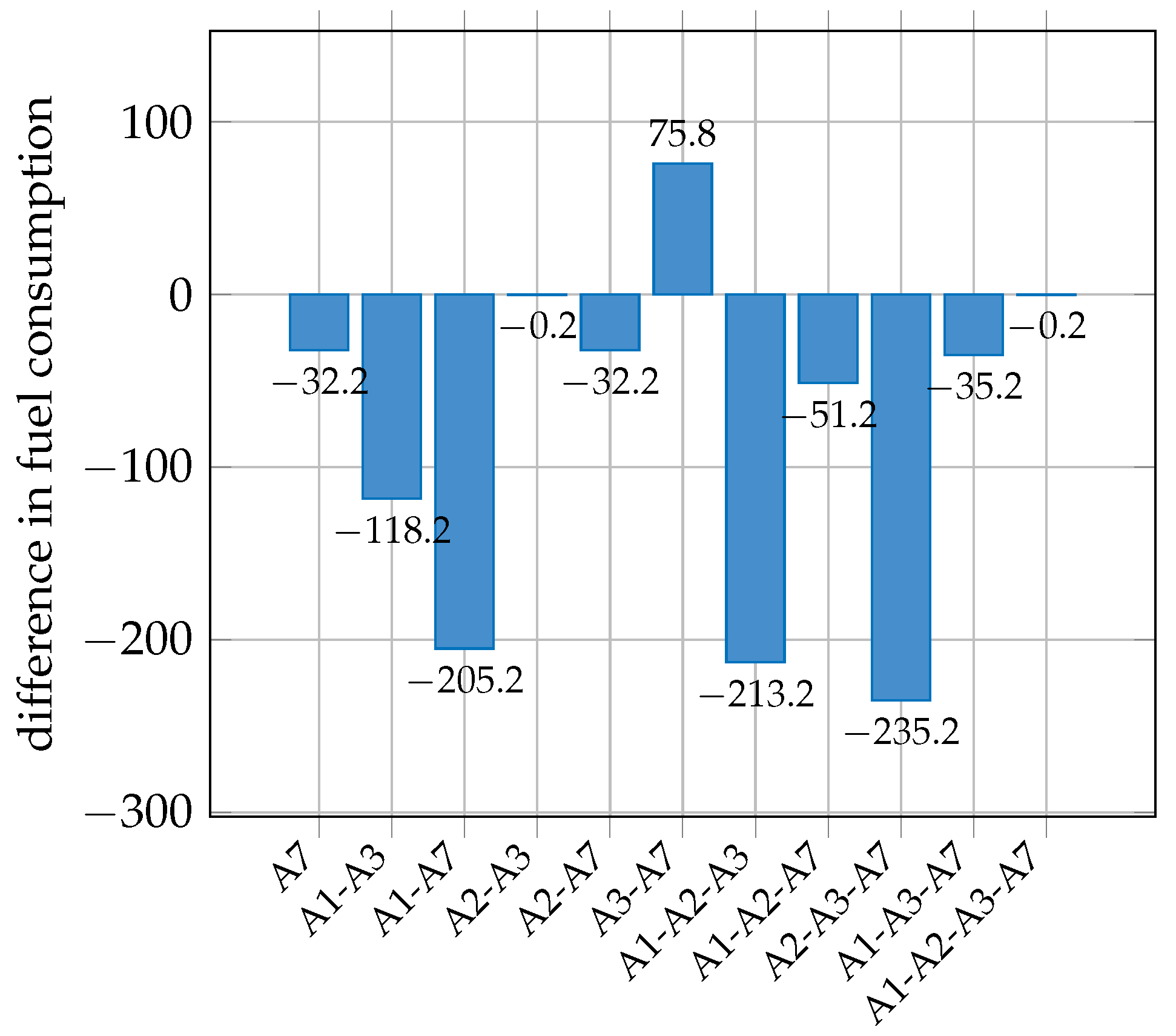
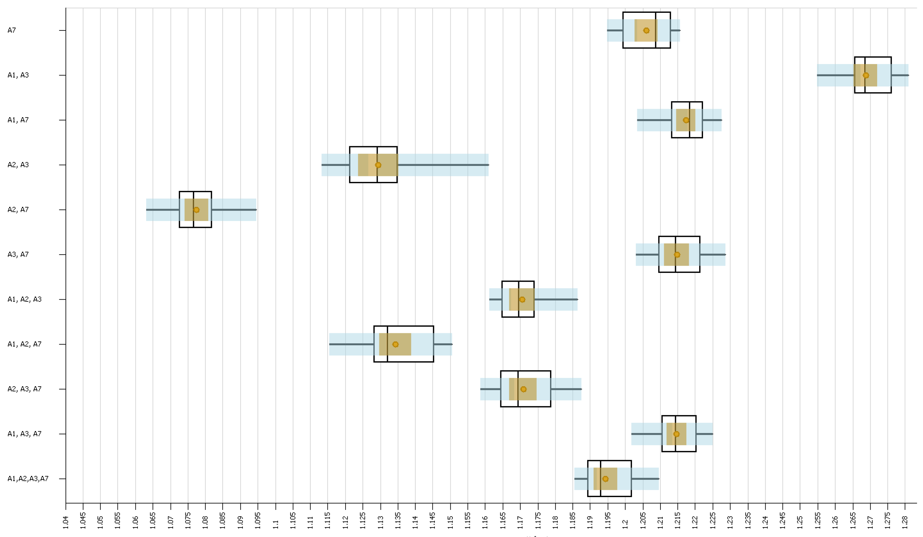
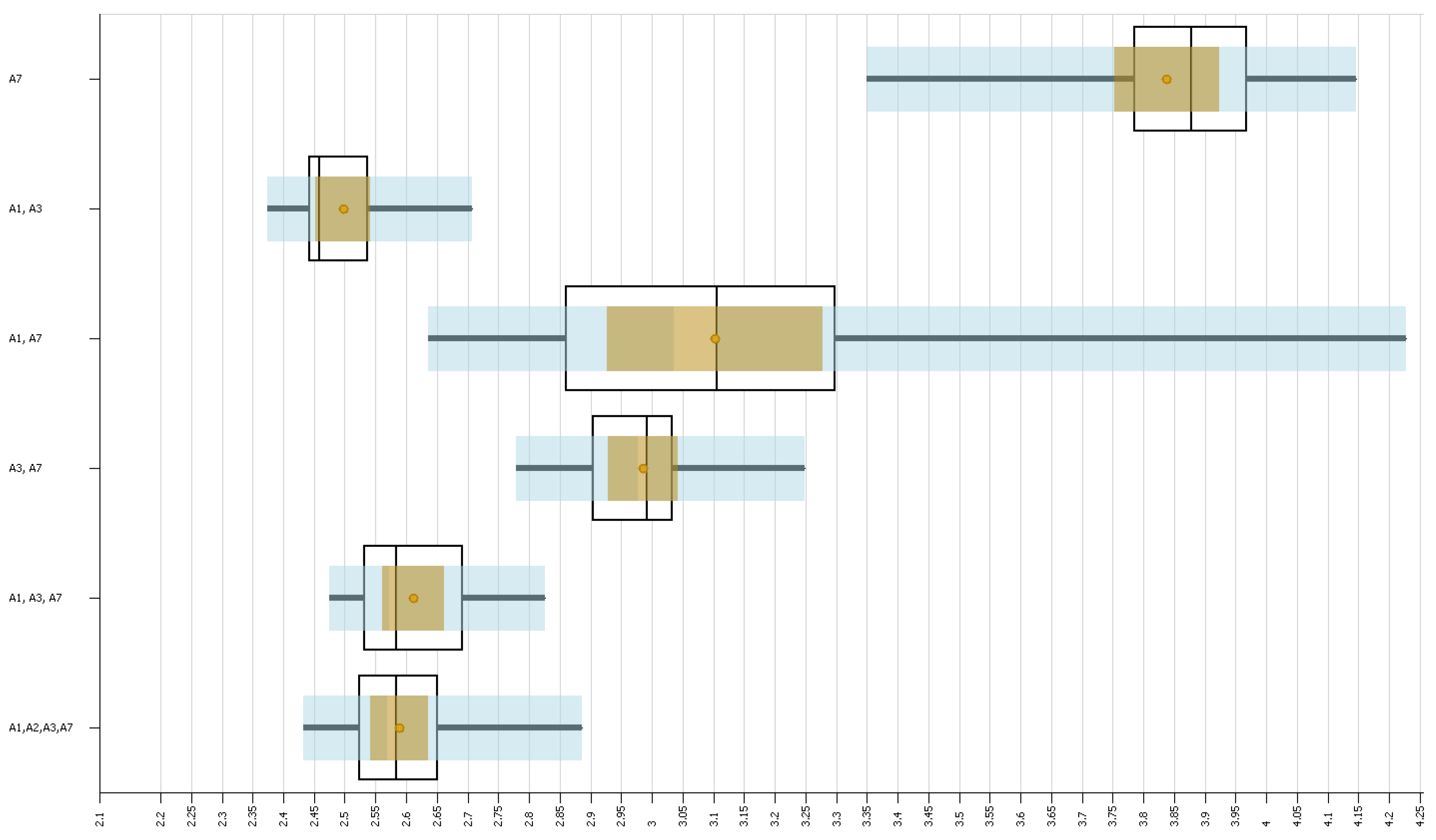
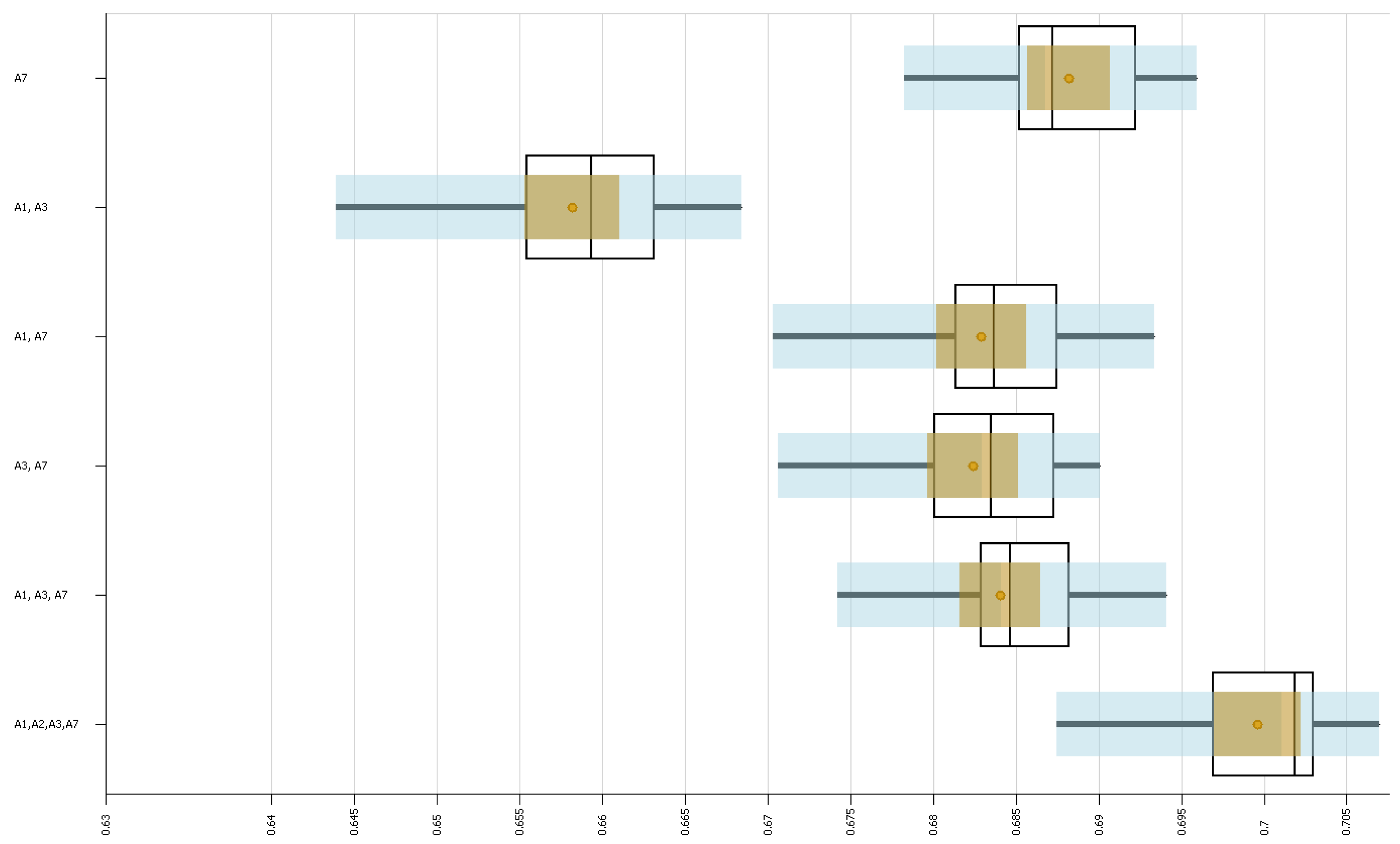
5.5. Third Experiment

The objective of this experiment was to understand the effect that different combinations of routes would have on the system. For this, we designed various scenarios in which different combinations of routes were used. Here, we only considered the routes that ran exclusively on Line 1 (see Table 1). Also, we only considered the combinations of routes that ensured that all stations were within reach using at least one combination of routes. We considered the following combinations:

• A7
• A1 and A3;
• A1 and A7;
• A2 and A3;
• A2 and A7;
• A3 and A7;
• A1, A2, and A3;
• A1, A2, and A7;
• A1, A3, and A7;
• A2, A3, and A7;
• A1, A2, A3, and A7.

In this experiment, our aim was for the total fuel consumption in the simulation to be as close as possible to 38,032.20 L (see Section 6.1), which is the value obtained in the experiment described in Section 5.3. To achieve this, we simply added enough buses to the routes in each scenario so that the total fuel consumption stayed the same in each hour using cross-multiplication.

For this experiment, we considered 11 scenarios, each with one of the combinations of routes described above. We ran each scenario 20 times and ran the simulation for 21 h in the same way as in the previous experiment.

6. Output Analysis

In this section, we will describe the performance of the output analysis of the experiments we conducted. Here, we will evaluate the current performance of the system and analyze the response to different control values. Our primary focus will be on the response variables defined in Section 5.2. Also, our objective is to provide information on the variables that can be changed to optimize the passenger satisfaction and also increase the system efficiency.

6.1. First Experiment’s Results

As described in Section 5.3, we first examined the current state of the system.

Table 2. Results of the response variables in the experiment described in Section 5.3.

	Mean	Minimum	Maximum	Half-With
Average satisfaction	1.1951	1.18	1.2096	0.0022
Average total fuel consumption (liters)	38,032.196	38,032.196	38,032.196	0
Average max Occupancy	0.6988	0.6875	0.7113	0.0018
Average queue satisfaction	0.8938	0.8884	0.9022	0.0009
Average bus occupancy	0.5696	0.5569	0.58	0.0017
Average queue length (minutes)	2.5946	2.4178	2.8863	0.0331

shows the results obtained in the first experiment. It should be noted that the half-widths of the confidence intervals were calculated using a 95% confidence level.

It should be noted that, as described in Section 5.2.2, the half-width of the average fuel consumption was 0, since this value is completely deterministic. Also, since all the confidence intervals were considerably small, we did not consider it necessary to perform more scenario replications in the following experiments.

6.2. Second Experiment’s Results

Now, we show the results of experiment Section 5.4. The goal of this experiment was to understand the changes in passenger satisfaction given increments in the total number of buses in the system.

As can be seen in Figure 6, the satisfaction response variable appeared to have an asymptotic behavior; this is natural because of the way that we defined this variable in Section 5.2.1, but it is interesting to see that it appears to have a maximum at 1.7 rather than 2. This is because the maximum occupancy also seemed to behave asymptotically towards 0.3, and the queue satisfaction grew toward 1, which is its maximum value by definition, as defined in Section 5.2.1. Also, by looking at Figure 7, we can conjecture that the maximum occupancy followed the law of diminishing returns [37], but this still needs to be proven outright.

If we look at the plot in Figure 8, is interesting to see that the average queue length seemed to be very sensitive to decreases in the total number of buses in the system, but it looks as though an increase of more than 20% in the total number of buses did not have a significant impact on the average queue lengths, since it also seemed to follow the law of diminishing returns [37].

Finally, the response variable, the total fuel consumption, is defined in the next equation:

$$T=m(38,032.20),$$

(10)

where T is the total fuel consumption, m represents the multiplier control variable, and 38,032.20 is the total fuel consumption when the multiplier is equal to 1; see Table 2. This is due to the deterministic nature of the total fuel consumption variable.

6.3. Third Experiment’s Results

As described in Section 5.5, the goal of this experiment was to understand the effects that different combinations of existing routes would have on the response variables.

Figure 9 shows us the difference in fuel consumption between scenarios; it can be seen that the biggest difference with respect to the value obtained from Table 2 was in scenario A2, A3, and A7, and the difference was 235.3 L, which is a difference of −0.006%, which we consider to be insignificant for the purpose of this experiment.

In Figure 10, the first thing we notice is that using only routes A1 and A3 yielded the most passenger satisfaction when using the same amount of resources. Furthermore, it is noticeable that that scenarios that include route A2 performed worse than those that did not. This is most likely because this route only covers the first 15 stations, since we were using cross-multiplication to adjust the number of buses and giving equal weights to all the routes in each scenario. Because of this, in scenarios where we considered A2, there were too many buses at the first 15 stations, which created a shortage of buses at the rest of the stations. Another interesting thing is that the scenario with the route A7 performed a little bit better than the original scenario (routes A1, A2, A3, and A7), but this may have been due to the influence of route A2.

As we can see in

Table 3. Table showing the response variable results for the experiment described in Section 5.5.

Scenario	T. Fuel Consumption	Satisfaction	M. Occupancy	Q. Satisfaction	B. Occupancy	Q. Length
A1,A2,A3,A7	38,032.20	1.19	0.70	0.89	0.57	2.59
A7	38,000.10	1.21	0.69	0.89	0.56	3.84
A1, A3	37,913.80	1.27	0.66	0.93	0.51	2.50
A1, A7	37,827.30	1.22	0.68	0.90	0.54	3.10
A2, A3	38,032.20	1.13	0.74	0.87	0.61	8.33
A2, A7	38,000.10	1.08	0.76	0.83	0.63	21.84
A3, A7	38,107.70	1.21	0.68	0.90	0.55	2.99
A1, A2, A3	37,819.40	1.17	0.71	0.88	0.57	7.25
A1, A2, A7	37,980.90	1.13	0.73	0.86	0.59	7.84
A2, A3, A7	37,796.90	1.17	0.72	0.89	0.59	3.23
A1, A3, A7	37,996.90	1.21	0.68	0.90	0.55	2.61

, the scenarios in which we considered route A2 performed poorly compared to the ones in which we did not consider it. This was most likely due to the circulation of too many buses only in the first 15 stations. Because of this, in the following plots regarding this experiment, we will not show those observations, which will allow for an easier reading of the plots.

In Figure 11, we can see the average queue length in minutes. It is interesting to see that, with respect to this response variable, the scenario with route A7 was outperformed by the original scenario by more than a minute. Again, the best-performing scenario was that with routes A1 and A3, but this was not by much.

Again, in Figure 12, we can see that the best-performing scenario was the one with routes A1 and A3, and the worst one was the original. Once again, we can see that the scenario with route A7 outperformed the original scenario, but this was most likely due to the original scenario including route A2.

Table 4. Table showing the response variable comparison between the original scenario plus 10% in total fuel consumption and the scenario in which we only considered routes A1 and A3.

Response	Original Scenario plus 10%	Scenario A1 and A3
Satisfaction	1.266	1.269
T. Fuel Consumption	41,835.416	37,913.796
Max. Occupancy	0.655	0.658
Queue Satisfaction	0.927	0.921
Avg. Occupancy	0.527	0.510
Queue Length	2.497	2.199

, shows a comparison between the scenario in which we considered routes A1 nd A3 with the scenario of the experiment described in Section 5.4, in which we increased the total number of buses by 10%. It is interesting that these two scenarios performed almost exactly the same, which shows us that there is a lot of room for improving the efficiency of the Metrobus system. It is likely that, if we consider scenarios in which we adjust the proportions of the buses on each of the routes, we could improve the efficiency of the system even more.

From this experiment, we can conclude a few things. First, it seems that the best option to maximize passenger satisfaction is to consider scenarios with routes that cover a larger part of the system (such as routes A1 and A3; check Table 1 and Table A1 for details), but that do not cover the entire system (such as route A7). In addition, it looks as though routes that travel to very few stations (such as route A2) are not effective in minimizing bus occupancy and queue lengths; this is most likely due to the law of diminishing returns, because a smaller number of buses will be sufficient, since the route is shorter. Lastly, it should be considered that if short routes are going to be considered, the total number of buses in these routes should be adjusted so that the system is not congested in those stations while having very few buses in the other stations.

7. Conclusions

In this paper, we have presented a model to simulate a BTR system that can be adapted to various fixed-route public transport systems. We focused on the Metrobus of CDMX, more specifically Line 1 of this system, and the connections it has to other lines in the system. We developed various response variables in order to evaluate the system’s performance, wherein we concentrated on the passenger satisfaction, measuring the maximum occupancy that a passenger experiences inside the buses, and the time he spends in the queues at the stations. We also calculated the total fuel consumption of the system in order to estimate the costs of the system and evaluate possible scenarios.

The results of the experiments showed us that it is possible to increase the passenger satisfaction in the system by increasing the total number of buses in the system, which increases the total fuel consumption, or by considering different combinations of routes and keeping the same fuel consumption. We have shown that considering only routes A1 and A3 increased the satisfaction levels for those observed when using 10% more resources. This indicates that it is possible to increase the satisfaction levels without using more buses than the ones already in use or by even reducing the number of buses while still obtaining an increase in satisfaction.

We showed that apparently passenger satisfaction follows the rule of diminishing returns; this result will be useful to perform optimizations in the future. Another important result we found is that it is more efficient to run the system with routes that do not transit in the full system; rather, they just transit in a fraction of this system, but it is important to note that if the route of these buses is too short, it has to be taken into account under the law of diminishing returns.

Future directions for research aimed at improving the quality of the BRT service, particularly with regard to the Mexico City Metrobus system, offer a wide range of possibilities. One of the most important things, from our point of view, is to evaluate new scenarios in which we consider new routes. This is because the results, shown in Section 6.3, showed that it is possible to increase passenger satisfaction by considering different combinations of routes without having to increase costs. One example of new routes that can be considered are “express routes”, in which the buses from these routes do not stop at every station that they pass through. This has been implemented with great success in TransMilenio, which is the BRT system that operates in Bogota, Colombia [38]. Another example could be to consider a combination of routes that minimize the passengers’ transfers, since passengers usually prefer to spend time riding the buses over making transfers [39].

Another direction is to develop a simpler model that replicates the result shown by our model, but with less computational power and with fewer built-in control variables. This will allow us to run simulations faster, which, ultimately, will allow us to perform optimization of the response variables. For example, in our model, the time between any two stations was sampled from an empirical probability distribution, which really affects the performance of the simulation. Also, our model considers 189 control variables, thereby making it difficult to create new scenarios, since all these variables must be considered. As mentioned in [40,41], simulation optimization methods are based on creating scenarios from the results of previous experiments; this makes a slow model with many decision variables not ideal for optimization.

Moreover, another aspect we consider interesting to explore is to simulate the user mix matrix U at different moments of the day to consider that the flow of passengers may change depending on the hour of the day. This is because it is very likely that passengers who go in one direction in the morning (generally to go to work or school) have to go back in the opposite direction (generally to their homes) in the afternoon. This could be achieved by defining a prior distribution $A_i$, where i represents the ith time interval of the day, which represents our belief in the directions that the passengers will follow. Then, we can use the same method that we described in Section 3.3 to simulate the matrix $U_i$ at the beginning of each time period. The methods for assessing the choice of prior distributions are presented in [42].