Abstract
Copula analysis was created to explain the dependence of two or more quantitative variables. Due to the need for in-depth data analysis involving complex variable relationships, there is always a need for new copula models with original features. As a modern example, for the analysis of circular or periodic data types, trigonometric copulas are particularly attractive and recommended. This is, however, an underexploited topic. In this article, we propose a new collection of eight trigonometric and hyperbolic copulas, four based on the sine function and the others on the tangent function, all derived from the construction of the famous Farlie–Gumbel–Morgenstern copula. In addition to their original trigonometric and hyperbolic functionalities, the proposed copulas have the feature of depending on three parameters with complementary roles: one is a dependence parameter; one is a shape parameter; and the last can be viewed as an angle parameter. In our main findings, for each of the eight copulas, we determine a wide range of admissible values for these parameters. Subsequently, the capabilities, features, and functions of the new copulas are thoroughly examined. The shapes of the main functions of some copulas are illustrated graphically. Theoretically, symmetry in general, stochastic dominance, quadrant dependence, tail dependence, Archimedean nature, correlation measures, and inference on the parameters are investigated. Some copula shapes are illustrated with the help of figures. On the other hand, some two-dimensional inequalities are established and may be of separate interest.
Keywords:
copulas; dependence models; trigonometric functions; hyperbolic functions; inequalities; correlation MSC:
60E15; 62H99
1. Introduction
In many real-world scenarios, modeling the relationship (or dependence) between two or more quantitative variables is crucial. In order to achieve this, the copulas provide effective solutions in the quantitative case. They recently received a lot of attention due to the varying intricacy of dependence that emerges in current data analysis challenges. An overview of the copula theory can be found in [1,2,3,4,5]. Two-dimensional copulas must be used when there are only two quantitative variables of concern. The following mathematical basis provides a definition of such two-dimensional copulas in the absolutely continuous case.
Definition 1.
(Absolutely continuous two-dimensional copulas [5]). Let . A two-dimensional function , , is said to be an absolutely continuous two-dimensional copula if and only if the following conditions are met for any :
- (I)
- and ,
- (II)
- and ,
- (III)
- , where represents the standard mixed second order partial derivatives according to x and y.
In the following, the mention “absolutely continuous two-dimensional” is omitted to lighten the comments. Clearly, from a technical viewpoint, the less immediate item in Definition 1 is item (III). It can demand fastidious developments.
Established families of copulas include the elliptical copulas (Gaussian, Student, etc.), Archimedean copulas (Ali–Mikhail–Haq, Clayton, Frank, etc.), extreme value copulas, and Farlie–Gumbel–Morgenstern (FGM)-type copulas. Despite the extensive literature, copula modeling is still a hot topic, and numerous research studies have been conducted to develop the approach from both the theoretical and practical aspects. Significant contemporary references include [6,7,8,9,10,11,12,13,14,15,16,17,18].
In order to motivate the findings of this article, a review of the FGM copula is required. To start, it is mathematically described as
where . In this expression, the polynomial function is considered a perturbed function of , and corresponds to the independence copula; when , is reduced to the independence copula. The key details about the FGM copula are contained in [1,2,3,4,5,19]. The polynomial form of the perturbation function and the moderate correlation range are two drawbacks of the FGM copula. These factors are crucial, among other situations, when fitting two-dimensional data. The FGM copula has, however, garnered a lot of attention from researchers due to its straightforward algebraic characteristics. It has also motivated new varieties of FGM-type copulas. See, for instance, [12,20,21,22].
On the other hand, recent references have suggested including trigonometric functions in the construction of copulas, making them more suitable in some circumstances. In particular, in order to model the correlations into phenomena that have a periodic, circular, or seasonal nature, it is intended to give the copula some oscillating properties. They are particularly well adapted to the correlation analysis of movement, circular, and environmental data. The references for conventional trigonometric copulas include [7,23,24,25,26,27,28,29]. For their practical aspect, we refer to [16,30,31,32,33]. Additionally, the trigonometric copulas now have a new applied dimension thanks to the R package Cylcop, recently created in [34].
In this article, we create a collection of new three-parameter copulas that have the general form of the FGM copula, but the perturbed function is completely redefined; it involves either trigonometric or hyperbolic functions. More precisely, we focus on special copulas of the following form:
where is the considered three-parameter vector and is a specific trigonometric or hyperbolic sine or tangent function. More precisely, the following functions for are considered:
The main novelties of the resulting copulas are in (i) the inclusion of a shape parameter that modulates the effect of on the perturbation function, following the spirit of the method in [12] for the extended FGM copula, (ii) the consideration of completely new trigonometric or hyperbolic functions for as the main transformation, and (iii) the consideration of the parameter , which is major to exploit at the maximum support of ; it can be considered an angle parameter if is a trigonometric function (see [7,26]). It is also worth noting that the perturbation function is not separable in x and y, i.e., we cannot write it as , where and denote two functions. For the common separable case, we may refer to [14], and the references therein.
In this innovative setting, for each of the eight copulas, we establish wide admissible ranges of values for , and , which may be connected in a sophisticated manner. The proofs are based on complex two-dimensional differentiations, factorizations, and various kinds of mathematical inequalities. The features of the suggested copulas are then investigated. The effect of the parameters on the shapes of some of them is illustrated graphically. In addition, the related functions (survival copula and copula density), symmetry (diagonal symmetry and radial symmetry), quadrant dependence, first-order stochastic dominance, tail dependence, medial and Spearman correlations are examined. The inference on the parameters is also briefly discussed. This study serves as the foundation for the development of new multi-dimensional trigonometric and hyperbolic copulas, which continue to be of particular relevance in various applications. On the other hand, a number of two-dimensional inequalities are discovered and might be of independent interest.
2. A Collection of Eight New Copulas
This section describes the created copulas in detail, as well as the main functions associated with them.
2.1. Sine-FGM Copula
The result below presents a new sine-FGM-type copula.
Proposition 1.
Let us consider the following two-dimensional function:
where , and α, β and γ are such that , , and
where . Then, is a copula.
Proof.
The proof consists in demonstrating that the proposed function satisfies the items (I), (II) and (III) of Definition 1.
- (I)
- For any , since , we haveUsing a similar development, for any , we obtain .
- (II)
- For any , we haveSimilarly, for any , it is clear that .
- (III)
- After differentiation, simplifications and factorizations, for any , we findHence, by manipulating the absolute values, the following inequality is obtained:Since and , we have and , so .Furthermore, since , we havewhereIn addition, since , we have . On the other hand, for any , we obviously have and . These results imply thatOwing to the following trigonometric inequalities, and for any , we haveSince and , it is clear that , and we haveBy combining the above inequalities, we obtainFinally, the assumption givesItem (III) is proved.
The proof of Proposition 1 ends. □
The copula shown in Equation (1) is named the sine-FGM (S) copula.
Remark 1.
Due to the numerous formulas involving the sine function, various equivalent expressions for the S copulas are possible. For instance, by using the formula for , an alternative expression is
The sine and cosine functions are thus involved.
Based on Equation (1), the S copula density is calculated as
Clearly, the parameter has a strong effect on the function at the extreme points , , and , which modifies the global morphology. We can examine the modeling potential of the S copula as well as the effects of the parameters , and on its shapes by looking at the forms of this function. A graphical analysis of the S copula and the S copula density is performed in Section 3.
As a complementary copula function, the S survival copula is given by
The main difference between the S copula and the S survival copula is the effect of , which is not the same. The S survival copula is also a novel three-parameter copula to be included in the body of the existing literature.
In a similar vein, we can present two new copulas based on the flipping method, thanks to the work of [35]; the x-flipping copula is specified as
and the y-flipping copula is specified as
For the sake of clarity, only the corresponding survival copulas are described for the remaining trigonometric and hyperbolic copulas.
Remark 2.
The coming proofs associated with the new copulas follow the main structure of the proof of Proposition 1, but the mathematical developments necessitate different approaches in terms of differentiation, factorization, and inequality tools, yielding a wide range of values for the parameters α, β, and γ.
2.2. Arcsine-FGM Copula
A novel copula of the arcsine-FGM type is shown in the result below. We recall that the arcsine of x, denoted as , is defined as the inverse sine function of x when . Moreover, we have .
Proposition 2.
Let us consider the following two-dimensional function:
where , and α and γ are such that , and
where . Then is a copula.
Proof.
The proof is based on Definition 1; the goal is to demonstrate that the proposed function satisfies the related items (I), (II) and (III).
- (I)
- For any , since , we haveUsing a similar development, for any , we obtain .
- (II)
- For any , we haveClearly, for any , we have .
- (III)
- After differentiation, simplifications and factorizations, for any , we establish thatHence, with the use of absolute values, we obtain the following inequality:Since and , we have and , so . Furthermore, we have , , and since , we establish thatwhereBy combining the above inequalities, we obtainHence, under the assumption , we findItem (III) is proved.
The proof of the proposition ends. □
The copula indicated in Equation (4) is called the arcsine-FGM (AS) copula.
Based on Equation (4), the AS copula density is specified by
It is important to note that, in contrast to other new copulas, this copula density has a relatively manageable expression.
The AS survival copula is given by
It is another new three-parameter copula to be added to the body of literature.
2.3. Hyperbolic Sine-FGM Copula
An innovative hyperbolic sine-FGM type copula is shown in the result below. We recall that the hyperbolic sine of x, denoted as , is defined as with . Furthermore, we have , which corresponds exactly to the hyperbolic cosine function, denoted by .
Proposition 3.
Let us consider the following two-dimensional function:
where , and α, β and γ are such that , and
where . Then is a copula.
Proof.
The proof refers to items (I), (II) and (III) of Definition 1.
- (I)
- For any , since , we haveSimilarly, for any , we obtain .
- (II)
- For any , we haveAdditionally, for any , we have .
- (III)
- After differentiation, simplifications and factorizations, for any , we obtainHence, with the use of absolute values, we establish the following inequality:Since and , we have and , so . Furthermore, it is clear that, since , we have , and for , we have and . These results imply thatOwing to the hyperbolic inequality for any , we findSince and , it is clear that , and, because is increasing for , we obtainwhereBy putting the above inequalities together, we obtainFinally, the assumption givesItem (III) is proved.
The proof of the proposition ends. □
The copula indicated in Equation (6) is called the hyperbolic sine-FGM (HS) copula.
Remark 3.
An alternative expression of the HS copula involving the exponential function is
To begin, based on Equation (6), the HS copula density is calculated as
The HS survival copula is given by
The HS survival copula is also a novel three-parameter copula to be included in the body of existing literature.
2.4. Hyperbolic Arcsine-FGM Copula
Below is the result, which displays a brand-new copula of the hyperbolic arcsine-FGM type. We recall that the hyperbolic arcsine of x, denoted as , is defined as with . Moreover, we have .
Proposition 4.
Let us consider the following two-dimensional function:
where , and α, β and γ are such that , and
Then, is a copula.
Proof.
The proof is based on Definition 1; the objective is to show that the proposed function fulfills the associated items (I), (II) and (III).
- (I)
- For any , since , we haveUsing a similar development, for any , we obtain .
- (II)
- For any , we obtainClearly, for any , we have .
- (III)
- After differentiation, simplifications and factorizations, for any , the following expression is determined:Hence, with the use of absolute values, we obtain the following inequality:Since and , we have and , so . Furthermore, we have , , and, obviously, . By combining the above inequalities, along with the assumption , we obtainItem (III) is proved.
This completes the proof of Proposition 4. □
The copula shown in Equation (8) is named the hyperbolic arcsine-FGM (HAS) copula.
Remark 4.
An alternative expression of the HAS copula involving the logarithmic function is
Based on Equation (8), the HAS copula density is calculated as
The HAS copula and copula density have the advantages of having weak constraints on the parameters (as indicated in Equation (9)), and manageable analytical expressions. For these reasons, a graphic analysis is devoted to them in Section 3.
The HAS survival copula is given by
Another brand-new three-parameter copula to be added to the corpus of current research is the HAS survival copula.
2.5. Tangent-FGM Copula
The result below exhibits a novel tangent-FGM type copula. We recall that the tangent function of x, denoted as , is defined as with x such that . Moreover, we have , where .
Proposition 5.
Let us consider the following two-dimensional function:
where , and α, β and γ are such that , and
where . Then is a copula.
Proof.
For this proof, it is enough to show that the items (I), (II) and (III) of Definition 1 are fulfilled.
- (I)
- For any , since , we haveUsing a similar argument, for any , we have .
- (II)
- For any , it is clear thatIn addition, for any , we have .
- (III)
- After differentiation, simplifications and factorizations, for any , we findHence, by using the absolute value properties, we obtainSince and , we have and , so . Furthermore, it is clear that . On the other hand, we have andwhereSince (strict inequality), we have . Since , , and and are increasing for , we obtainandThe above inequalities giveFinally, the assumption implies thatThe item (III) is proved.
The proof of the proposition ends. □
The copula shown in Equation (11) is named the tangent-FGM (T) copula.
Based on Equation (11), the T copula density is calculated as
The T survival copula is given by
The T survival copula is also a novel three-parameter copula to be included in the body of existing literature.
2.6. Arctangent-FGM Copula
The result shown below exhibits a distinctive copula of the arctangent-FGM type. We recall that the arctangent function of x, denoted as , is defined as the inverse tangent function of x when . Moreover, we have .
Proposition 6.
Let us consider the following two-dimensional function:
where , and α, β and γ are such that , and
Then is a copula.
Proof.
The proof is based on Definition 1; we aim to demonstrate that the proposed function satisfies the related items (I), (II) and (III).
- (I)
- For any , since , we haveSimilarly, for any , we obtain .
- (II)
- For any , we obviously haveIn addition, for any , we obtain .
- (III)
- After differentiation, simplifications and factorizations, for any , we findHence, with the use of absolute values, we haveSince and , we have and , so . In addition, it is clear that and . Furthermore, we havewhereHence, the assumptions and imply that andThe above inequalities and the assumption yieldItem (III) is proved.
The proof of the proposition ends. □
The copula shown in Equation (13) is named the arctangent-FGM (AT) copula.
Based on Equation (13), the AT copula density is calculated as
The AT survival copula is given by
The AT survival copula is also a novel three-parameter copula to be included in the body of existing literature.
2.7. Hyperbolic Tangent-FGM Copula
A unique hyperbolic tangent-FGM type copula can be seen in the result below. We recall that the hyperbolic tangent function of x, denoted as , is defined as when . In addition, we have , which corresponds to the square of the hyperbolic secant function, denoted by , i.e., .
Proposition 7.
Let us consider the following two-dimensional function:
where , and α, β and γ are such that , and
with such that , i.e., . Then is a copula.
Proof.
The objective is to demonstrate that the proposed function satisfies the items (I), (II) and (III) of Definition 1.
- (I)
- For any , since , we obtainUsing a similar development, for any , we have .
- (II)
- For any , we haveAdditionally, for any , it is clear that .
- (III)
- After differentiation, simplifications and factorizations, for any , we obtainHence, the following inequalities are established with the use of absolute values:Since and , we have and , so . Furthermore, it is clear that . On the other hand, since , we havewhereOwing to the assumption , we obtain . Let us now set . Since for , is decreasing and we have , so . This implies thatSince is decreasing for , with , we have .The above inequalities and the assumption giveItem (III) is proved.
Proposition 7 is proved. □
The copula shown in Equation (15) is named the hyperbolic tangent-FGM (HT) copula.
Remark 5.
An alternative expression of the HT copula involving the exponential function is
Based on Equation (15), the HT copula density is calculated as
The HT survival copula is given by
Another new three-parameter copula to be added to the body of current research is the HT survival copula.
2.8. Hyperbolic Arctangent-FGM Copula
A remarkable copula of the hyperbolic arctangent-FGM type is proposed in the result given below. We recall that the hyperbolic arctangent function of x, denoted as , is defined as when . Moreover, we have .
Proposition 8.
Let us consider the following two-dimensional function:
where , and α, β and γ are such that , and
where . Then is a copula.
Proof.
The proof is based on Definition 1; we need to show that the proposed function satisfies the related items (I), (II) and (III).
- (I)
- For any , since , we haveSimilarly, for any , we obtain .
- (II)
- For any , we haveMoreover, for any , we have .
- (III)
- After differentiation, simplifications and factorizations, for any , the following expression is obtained:Hence, with the use of absolute values, we establish the following inequality:Since and , we have and , so . Furthermore, we have ,andwhereHence, under the assumption (strict inequality), we obviously have . The above inequalities giveThe assumption implies thatItem (III) is proved.
The proof of the proposition ends. □
The copula shown in Equation (17) is named the hyperbolic arctangent-FGM (HAT) copula.
Remark 6.
An alternative expression of the HAT copula involving the logarithmic function is
Based on Equation (17), the HAT copula density is calculated as
The HAT survival copula is given by
The HAT survival copula is a brand-new three-parameter copula to be added to the corpus of current research.
Some graphical and analytical characteristics of the proposed copulas are the focus of the remaining sections of the article.
3. Graphics and Properties
This section contains a short graphical copula analysis and a unified study of the proposed copulas.
3.1. Graphical Analysis of The S Copula
We examine the shapes of two particular copulas, the S and HAS copulas, in order to emphasize the importance of our findings. After some preliminary tests, certain parameter values will be chosen from the list of acceptable values and according to their impact on the shapes.
We begin with the S copula as defined by (1). First, a simplified configuration is considered: , which gives . The conditions in Proposition 1, i.e., in Equation (2), yield and
Let us now explore the effect of on the shapes of the S copula and the S copula density, in turn.
For the first analysis, we arbitrarily chose . In this case, the condition on becomes .
In Figure 1, we plot the S copula as defined in Equation (1) with , and , satisfying the required conditions.
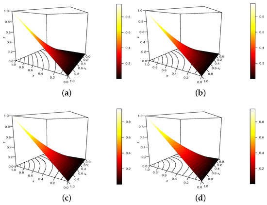
Figure 1.
Display of the S copula for , , and (a) , (b) , (c) and (d) .
We observe that the shapes of the copula are affected by the change in values of , which reveals a certain versatility. Moreover, it is clear that the conditions satisfied by a copula are fulfilled.
Figure 2 completes Figure 1: we plot the S copula density as defined in Equation (3) under the same configuration, i.e., , and .
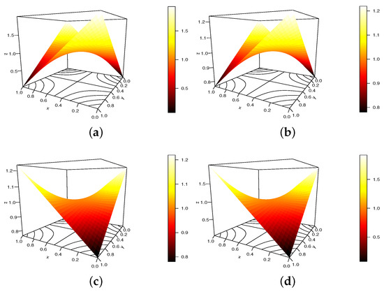
Figure 2.
Display of the S copula density for , , and (a) , (b) , (c) and (d) .
Again, we see that the changing values of have an impact on the morphologies of the shapes. Furthermore, it is evident that the mathematical requirements of a copula density are satisfied, particularly the positivity.
Let us now investigate the effect of on the shapes of the S copula and the S copula density.
We chose for numerical convenience. Then, the condition on becomes . Hence, we propose to fix and vary the values of .
In Figure 3, we plot the S copula with , and , satisfying the required conditions.
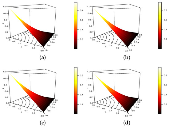
Figure 3.
Display of the S copula for , , and (a) , (b) , (c) and (d) .
The contour plot reveals a difference in lines and a difference in intensity in the red color zone, both of which show that the forms of the S copula are altered; this is evidence that has a shape effect.
In Figure 4, we plot the S copula density under the same configuration, i.e., , and .
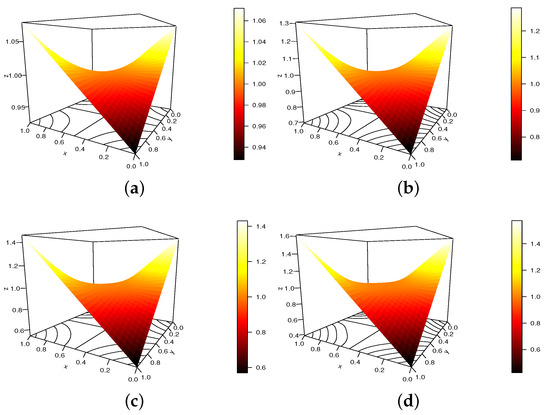
Figure 4.
Display of the S copula density for , , and (a) , (b) , (c) and (d) .
In this figure, the contour plot makes it easier to see the subtle changes in the copula density shapes. However, it is evident that the requirements for a legitimate copula density are met.
We end this graphical analysis with an example of . In this case, we have , and we can take as . With the arranging choice , we can take as .
In Figure 5, we plot the S copula with , and , satisfying the required conditions.
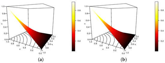
Figure 5.
Display of the S copula for , , and (a) and (b) .
The contour plot and the intensity of the red color zone are the key differences.
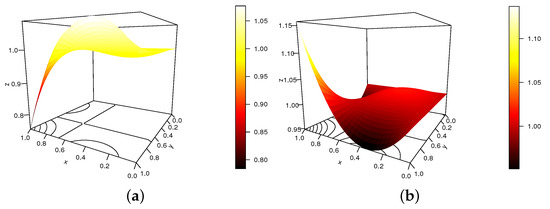
Figure 6.
Display of the S copula density for , , and (a) and (b) .
The shapes completely change in this figure because of the alternated sign. When , the restriction is applied and may present a challenge for flexible dependence modeling.
3.2. Graphical Analysis of the HAS Copula
One of our most important discoveries is the manageability of the HAS copula as defined in Equation (8), which only requires the following parameter conditions: , and . For this reason, we propose to study it from a graphical viewpoint.
To begin, let us replace by with , such that , to activate all the parameters in a straightforward manner. With this configuration, we define the HAS copula with only two varying parameters, and , but the values of have an effect on those of .
In Figure 7, we plot the HAS copula with , and , satisfying the required conditions.
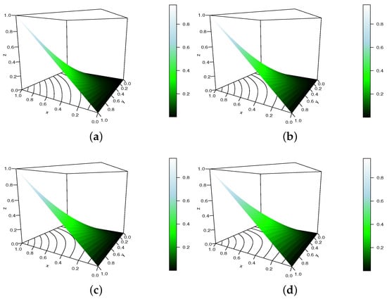
Figure 7.
Display of the HAS copula for , , and (a) , (b) , (c) and (d) .
In this figure, especially if we compare Figure 7a,d, we observe a wide change in the shapes of the HAS copula, indicating a significant effect of . This shows the versatility of the HAS copula in terms of shapes.
In Figure 8, we plot the HAS copula density as defined in Equation (10) under the same configuration, i.e., , and .
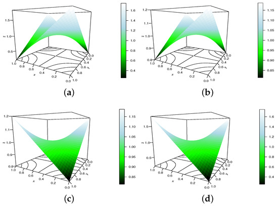
Figure 8.
Display of the HAS copula density for , , and (a) , (b) , (c) and (d) .
In this figure, positional differences are observed with various intensity values. Once again, the copula density meets the requirement in terms of assumptions, including positivity.
Let us now investigate the effect of on the shapes of the HAS copula and the HAS copula density, under the configuration . Let us fix and vary the values of .
In Figure 9, we plot the HAS copula with , and , satisfying the required conditions.
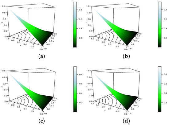
Figure 9.
Display of the HAS copula for , , and (a) , (b) , (c) and (d) .
In this figure, we also observe changes of morphologies, indicating that the copula shapes are dependent on the combined action of and .
In Figure 10, we plot the HAS copula density under the same configuration, i.e., , and .
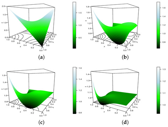
Figure 10.
Display of the HAS copula density for , , and (a) , (b) , (c) and (d) .
In some sense, Figure 10 supports Figure 9; the HAS copula produces a copula density very versatile in shapes.
To wrap up this section, we display figures to show that a few of the proposed copulas have the adaptability to be used in practical settings and produce applicable dependence models. Similar characteristics are seen for the other copulas as well, but for space reasons, we do not include their graphical analysis.
3.3. List of Properties
This section establishes some basic characteristics of the introduced copulas. We work with their general form, which involves the function , i.e.,
with
and and (which are common conditions in all of the preceding propositions). The theoretical details of the coming notions are all contained in [5].
To begin, the independence copula is always obtained by setting . The proposed copulas are diagonally symmetric because for any . They are not Archimedean because one can find many examples of triplet values such that
The non-Archimedean property is implied by the non-associativity of . Because of the change of the parameter , the considered copulas are not radially symmetric for and ; there exists such that . They are radially symmetric for or .
Of course, as a well-established copula fact, we have the Fréchet–Hoeffding bounds: for any , we have . As immediate consequences, the following two-dimensional inequalities involving hold: for any , we have
These inequalities can be of separate interest and serve as mathematical tools for various two-dimensional analyses.
Let us now look at the various quadrant dependence properties in relation to the parameters.
- For , it is clear that , implying that for any ; the considered copulas are positively quadrant dependent.
- For , it is clear that , implying that the reversed inequality holds: for any ; the considered copulas are negatively quadrant dependent.
In addition, some first-order copula orders with other copulas can be demonstrated. In particular, if satisfies for u in the support of , which is the case for , the results below are established.
- For , we have for any , whereIt is a copula that is an extended version of the FGM copula with the dependence parameters (see [12]).
- For , the reversed inequality holds: we have for any .
If satisfies for u in the support of , which is the case for , the reversed first-order copula orders hold.
The proposed copulas have tractable series expansions based on series expansions of with . Such expansions can express or approximate various crucial correlation measures, which makes them useful in particular situations.
Various kinds of tail dependence for the proposed copulas are examined below. Since all the considered functions satisfied when and , we have
Thus, the considered copulas have no lower tail dependence. Concerning the upper tail dependence, using similar arguments, we have
No upper tail dependence is determined. As a result, the suggested copulas are totally tail independent.
There exist many measures of correlation (see [5]). Among them are the medial correlation (or coefficient of Blomqvist) and the Spearman correlation. In our setting, there are investigated below.
The medial correlations of the considered copulas are given by the following general formula:
They are expressed for each of the eight copulas in Table 1.

Table 1.
Expressions of the medial correlations and series expansions of the Spearman correlations of the new copulas.
Some medial correlation orders can be established. In particular, if satisfies for u in the support of , which is the case for , then the results below hold.
- For , we have , where denotes the medial correlation of the copula given in Equation (19).
- For , the reversed inequality holds; we have .
If satisfies for u in the support of , which is the case for , the reversed medial correlation orders hold.
The Spearman correlations of the considered copulas are specified by the following general formula:
However, the series expansions for mentioned above can be used to obtain series expansions for . These expansions are given in Table 1. The standard beta function is defined in this table as with and (implemented in most of the mathematical software), the double factorial as (until 1 or 2, depending on the parity nature of n), and the Bernoulli numbers as .
Other well-known copula correlation measures can be expressed in a similar way (Gini gamma, Spearman footrule coefficient, etc.).
Some Spearman correlation orders can be established. In particular, if satisfies for u in the support of , which is the case for , then the results below follow.
- For , we have , where denotes the Spearman correlation of the copula given in Equation (19).
- For , the reversed inequality holds: we have .
If satisfies for u in the support of , which is the case for , the reversed Spearman correlation orders hold. Thus, the values of the Spearman correlations of the proposed copulas can be really versatile and go beyond those of the FGM copula (in the positive or negative sense). This reason, combined with the functionalities of , justifies the use of these copulas for applications where the FGM copula produces moderate or good results, for possible better modeling.
As a well-known copula fact, the proposed copulas can define new parametric two-dimensional distributions. In fact, by merging two uni-dimensional cumulative distribution functions, say and , we build a new two-dimensional cumulative distribution function as follows:
where represents the vector of all the involved parameters, i.e., and those in and . In [36], among other topics, the choices for motivated lifetime cumulative distribution functions are covered.
Finally, in a statistical scenario, we often need to estimate the unknown parameter vector from data. To this end, as for all copulas, we may think to use the “omnibus estimation method”, which can be described as follows. For a known integer n, let , be data drawn from a continuous random vector, say . Then, with the use of the proposed copulas and their respective copula densities, denoted generically here by , the omnibus estimate of is defined as
where
and refers to the indicator function over an event denoted as A. Therefore, after substituting the transformed data , , the omnibus estimate can be described as a fundamental maximum likelihood estimate of . This semi-parametric estimation technique aims to prevent potential marginal distribution misspecification, which could lead to an overestimation of the level of dependence in the data. The references [37,38] contain the theoretical guarantees of . Additional remarks on the perspectives of the applied aspects of the suggested copulas are provided in the section that follows.
4. Conclusions
4.1. Summary
In this article, we produced eight two-dimensional copulas by combining trigonometric and hyperbolic perturbation functions with a FGM copula structure, riding the wave of the emergence of new dependence models. They depend on three parameters, each of which plays an important role in various shape and correlation aspects.
To the best of our knowledge, all of the main copulas described in this article are brand new to the literature. For a summary view, they are listed in Table 2.

Table 2.
Copulas proposed in this article.
The trigonometric nature of some new copulas offers interesting perspectives for modeling circular-type dependence (see [31,33,34]). For each of the eight copulas, we identified wide ranges of acceptable parameter values. The proofs were given in full detail. Their capabilities were carefully examined. Figures were used to illustrate the shapes of the S and HAS copulas. Theoretically, the symmetry in general, stochastic dominance, quadrant dependence, tail dependence, Archimedean nature, and correlation measures were investigated. The inference on the parameters was discussed. As a result, the provided collections of copulas enhance the specialized literature and serve as the foundation for fresh dependence models for diverse theoretical or practical uses.
4.2. Limitations
- To obtain a wide range of acceptable values for the three parameters of the suggested copulas, every mathematical effort was made. However, we do not claim that these ranges are optimal in the strict sense. There is probably some (minor) room for improvement, but a solid mathematical basis is given in the article.
- It is worth noting that the article is mainly theory oriented, even though concrete models are provided with all the details necessary to be practically implemented. However, applications to real-world data are missing. This aspect requires experience and skills that go beyond what the author of this study currently have.
4.3. Perspectives
- The applied aspect is the logical sequel of this article. In particular, by their construction, our trigonometric copulas are interesting and logically recommended for the analysis of circular or periodic data types. This is the most recent interpretation of our findings. The creation of R packages for the proposed copula models similar to Cylcop (see [34]) is also a challenging project.
- Based on our two-dimensional copulas, we can consider building copulas of higher dimensions, particularly three-dimensional copulas, given their potential applications in diverse environmental models, etc. (see [39,40,41]). A natural three-dimensional extended form iswithand and .
These points need further investigation, which we will leave for future work.
4.4. Extra Remark
Finally, Table 3 shows some inequalities resulting from our copulas and survival copulas, and the associated Fréchet–Hoeffding bounds. To the best of our knowledge, these inequalities are new and might be of independent interest. We recall that, as minimum conditions, , and , and that .

Table 3.
Inequalities derived from the proposed copulas (and survival copulas).
Funding
This research received no external funding.
Institutional Review Board Statement
Not applicable.
Informed Consent Statement
Not applicable.
Data Availability Statement
Not applicable.
Acknowledgments
The author thanks the three reviewers, the associate editor and the editor for their constructive comments on the article.
Conflicts of Interest
The author declares no conflict of interest.
References
- Cuadras, C.M. The importance of being the upper bound in the bivariate family. SORT 2006, 30, 55–84. [Google Scholar]
- Durante, F.; Sempi, C. Principles of Copula Theory; CRS Press: Boca Raton, FL, USA, 2016. [Google Scholar]
- Joe, H. Dependence Modeling with Copulas; CRS Press: Boca Raton FL, USA, 2015. [Google Scholar]
- Nadarajah, S.; Afuecheta, E.; Chan, S. A compendium of copulas. Statistica 2017, 77, 279–328. [Google Scholar]
- Nelsen, R. An Introduction to Copulas, 2nd ed.; Springer Science+Business Media, Inc.: New York, NY, USA, 2006. [Google Scholar]
- Bekrizadeh, H.; Parham, G.; Jamshidi, B. A new asymmetric class of bivariate copulas for modeling dependence. Commun. Stat.-Simul. Comput. 2017, 46, 5594–5609. [Google Scholar] [CrossRef]
- Chesneau, C. Theoretical study of some angle parameter trigonometric copulas. Modelling 2022, 3, 140–163. [Google Scholar] [CrossRef]
- Chesneau, C. Theoretical contributions to three generalized versions of the Celebioglu-Cuadras copula. Analytics 2023, 2, 31–54. [Google Scholar] [CrossRef]
- Cuadras, C.M. Constructing copula functions with weighted geometric means. Stat. Plan. Inference 2009, 139, 3766–3772. [Google Scholar] [CrossRef]
- Diaz, W.; Cuadras, C.M. An extension of the Gumbel-Barnett family of copulas. Metrika 2022, 85, 913–926. [Google Scholar] [CrossRef]
- El Ktaibi, F.; Bentoumi, R.; Sottocornola, N.; Mesfioui, M. Bivariate copulas based on counter-monotonic shock method. Risks 2022, 10, 202. [Google Scholar] [CrossRef]
- Huang, J.S.; Kotz, S. Modifications of the Farlie-Gumbel-Morgenstern distributions. A tough hill to climb. Metrika 1999, 49, 135–145. [Google Scholar] [CrossRef]
- Manstavičius, M.; Bagdonas, G. A class of bivariate independence copula transformations. Fuzzy Sets Syst. 2022, 428, 58–79. [Google Scholar] [CrossRef]
- Rodríguez-Lallena, J.A.; Ubeda-Flores, M. A new class of bivariate’ copulas. Stat. Probab. Lett. 2004, 66, 315–325. [Google Scholar] [CrossRef]
- Saali, T.; Mesfioui, M.; Shabri, A. Multivariate extension of Raftery copula. Mathematics 2023, 11, 414. [Google Scholar] [CrossRef]
- Susam, S.O. A new family of archimedean copula via trigonometric generator function. Gazi Univ. J. Sci. 2020, 33, 795–802. [Google Scholar] [CrossRef]
- Roberts, D.J.; Zewotir, T. Copula geoadditive modelling of anaemia and malaria in young children in Kenya, Malawi, Tanzania and Uganda. J. Health Popul. Nutr. 2020, 39, 8. [Google Scholar] [CrossRef]
- Yang, Y.; Li, S. On a family of log-gamma-generated Archimedean copulas. N. Am. Actuar. J. 2022, 26, 123–142. [Google Scholar] [CrossRef]
- De La Horra, J.; Fernandez, C. Sensitivity to prior independence via Farlie-Gumbel-Morgenstern model. Commun. Stat.-Theory Methods 1995, 24, 987–996. [Google Scholar] [CrossRef]
- Bayramoglu, K.; Bayramoglu (Bairamov), I. Baker- Lin-Huang type bivariate distributions based on order statistics. Commun. Stat.-Theory Methods 2014, 43, 1992–2006. [Google Scholar] [CrossRef]
- Dolati, A.; Úbeda-Flores, M. Constructing copulas by means of pairs of order statistics. Kybernetika 2009, 45, 992–1002. [Google Scholar]
- Lai, C.D.; Xie, M. A new family of positive quadrant dependent bivariate distributions. Stat. Probab. Lett. 2000, 46, 359–364. [Google Scholar] [CrossRef]
- Alfonsi, A.; Brigo, D. New families of copulas based on periodic functions. Commun. Stat.-Theory Methods 2005, 34, 1437–1447. [Google Scholar] [CrossRef]
- Amblard, C.; Girard, S. Symmetry and dependence properties within a semiparametric family of bivariate copulas. J. Nonparametric Stat. 2002, 14, 715–727. [Google Scholar] [CrossRef]
- Chesneau, C. A study of the power-cosine copula. Open J. Math. Anal. 2021, 5, 85–97. [Google Scholar] [CrossRef]
- Chesneau, C. On new types of multivariate trigonometric copulas. AppliedMath 2021, 1, 3–17. [Google Scholar] [CrossRef]
- Chesneau, C. A note on a simple polynomial-sine copula. Asian J. Math. Appl. 2022, 2, 1–14. [Google Scholar]
- Durante, F. A new class of symmetric bivariate copulas. J. Nonparametric Stat. 2006, 18, 499–510. [Google Scholar] [CrossRef]
- Jones, M.C.; Pewsey, A.; Kato, S. On a class of circulas: Copulas for circular distributions. Ann. Inst. Stat. Math. 2015, 67, 843–862. [Google Scholar] [CrossRef]
- Davy, M.; Doucet, A. Copulas: A new insight into positive time-frequency distributions. IEEE Signal Process. Lett. 2003, 10, 215–218. [Google Scholar] [CrossRef]
- Hodel, F.H.; Fieberg, J.R. Circular-linear copulae for animal movement data. Methods Ecol. Evol. 2022, 13, 1001–1013. [Google Scholar] [CrossRef]
- Knockaert, L. A class of positive isentropic time-frequency distributions. IEEE Signal Process. Lett. 2002, 9, 22–25. [Google Scholar] [CrossRef]
- Xiao, Q.; Zhou, S.W. Modeling correlated wind speeds by trigonometric Archimedean copulas. In Proceedings of the 11th International Conference on Modelling, Identification and Control (ICMIC2019), Tianjin, China, 13–15 July 2019; Wang, R., Chen, Z., Zhang, W., Zhu, Q., Eds.; Lecture Notes in Electrical Engineering. Springer: Singapore, 2020; Volume 582. [Google Scholar]
- Hodel, F.H.; Fieberg, J.R. Cylcop: An R package for circular-linear copulae with angular symmetry. BioRxiv 2021. [Google Scholar] [CrossRef]
- De Baets, B.; De Meyer, H.; Kalická, J.; Mesiar, R. Flipping and cyclic shifting of binary aggregation functions. Fuzzy Sets Syst. 2009, 160, 752–765. [Google Scholar] [CrossRef]
- Taketomi, N.; Yamamoto, K.; Chesneau, C.; Emura, T. Parametric distributions for survival and reliability analyses, a review and historical sketch. Mathematics 2022, 10, 3907. [Google Scholar] [CrossRef]
- Genest, C.; Ghoudi, K.; Rivest, L.P. A semiparametric estimation procedure of dependence parameters in multivariate families of distributions. Biometrika 1995, 82, 543–552. [Google Scholar] [CrossRef]
- Silvapulle, P.; Kim, G.; Silvapulle, M.J. Robustness of a semiparametric estimator of a copula. Econom. Soc. 2004, 317. [Google Scholar]
- Hui-Mean, F.; Yusof, F.; Yusop, Z.; Suhaila, J. Trivariate copula in drought analysis: A case study in peninsular Malaysia. Oretical Appl. Climatol. 2019, 138, 657–671. [Google Scholar] [CrossRef]
- Orcel, O.; Sergent, P.; Ropert, F. Trivariate copula to design coastal structures. Nat. Hazards Earth Syst. Sci. 2020, 21, 239–260. [Google Scholar] [CrossRef]
- Úbeda Flores, M. A method for constructing trivariate distributions with given bivariate margins. Far East J. Theor. Stat. 2005, 15, 115–120. [Google Scholar]
Disclaimer/Publisher’s Note: The statements, opinions and data contained in all publications are solely those of the individual author(s) and contributor(s) and not of MDPI and/or the editor(s). MDPI and/or the editor(s) disclaim responsibility for any injury to people or property resulting from any ideas, methods, instructions or products referred to in the content. |
© 2023 by the author. Licensee MDPI, Basel, Switzerland. This article is an open access article distributed under the terms and conditions of the Creative Commons Attribution (CC BY) license (https://creativecommons.org/licenses/by/4.0/).