Abstract
Shor’s algorithm for prime factorization is a hybrid algorithm consisting of a quantum part and a classical part. The main focus of the classical part is a continued fraction analysis. The presentation of this is often short, pointing to text books on number theory. In this contribution, we present the relevant results and proofs from the theory of continued fractions in detail (even in more detail than in text books), filling the gap to allow a complete comprehension of Shor’s algorithm. Similarly, we provide a detailed computation of the estimation of the probability that convergents will provide the period required for determining a prime factor.
1. Introduction
Shor’s algorithm [1] for prime factorization is generally considered as a major milestone and a breakthrough in quantum computing: it solves a practically very relevant problem (which is, e.g., an underpinning of cryptography) with an exponential speedup compared to classical methods.
The algorithm is based on the fact that determining a divisor and finally a prime factor of a natural number can be reduced to finding the period p of the modular exponentiation function for an a with (see Section 3.2.1).
The overall algorithm is hybrid, consisting of classical computations and a quantum computation. The classical computations are computing greatest common divisors with the Euclidian algorithm, and perform a continuous fraction analysis. A detailed discussion of the latter is one of the two foci of this contribution (see Section 2).
The quantum part mainly consists of: (i) creating an entangled state based on an oracle computing the modular exponentiation function f above, (ii) performing a quantum Fourier transform (QFT) on this state, and (iii) measuring it. The oracle produces the following state:
After applying the quantum Fourier transform and a measurement, the first part (i.e., the |a⟩-part) of the quantum register is in state
In this state, the searched period p already appears in its amplitude. The measured value y can then be used with high probability (see Section 3.4, Theorem 16) to compute the period p of the modular exponentiation function f by analyzing the convergents of a continued fraction (see Section 3.4.1) and finally, based on the period, a prime factor (see Section 3.2.1). A detailed discussion on how this is achieved is the second focus of this contribution (see Section 3).
Structure of the Article
The article is structured as follows: in Section 2 we cover all details about continued fractions that are required to comprehend the corresponding aspect of Shor’s algorithm.
Section 2.1 defines the notion of a continued fraction, gives examples of how to compute the continued fraction representation of a rational number, and demonstrates how to compute the number that a continued fraction (and thus convergents) represents.
Convergents as the fundamental tool in the theory of continued fractions are detailed in Section 2.2: after defining the term, basic theorems about convergents such as the recursion theorem, two sign theorems, monotony properties, convergent comparison, nesting of a number by its convergents, and several distance estimations are proven.
Next, the brief Section 2.3 presents infinite regular continued fractions to represent non-rational numbers. A corresponding algorithm is provided to compute such continued fractions.
Section 2.4 gives several upper bounds and lower bounds for the difference between a number and its convergents. Exploiting one of these bounds, the convergence of the convergents of an infinite regular continued fraction of a number to this number is proven. Semiconvergents are defined and corresponding monotony properties are given.
Best approximations of a real number are introduced in Section 2.5. It is proven that best approximations of the second kind are convergents and vice versa (Lagrange’s theorem). Best approximations of the first kind are proven to be convergents or semiconvergents (another theorem by Lagrange). Finally, Legendre’s theorem is presented, which is the main result about continued fractions required by Shor’s algorithm: it allows the implication that a given fraction is a convergent of another number.
Section 3 is devoted to estimating the probability that convergents can be used to compute periods, i.e., that Legendre’s theorem can be applied.
At the beginning of Section 3, Section 3.1 proves a lower bound and an upper bound for the secant lengths of the unit circle. This estimation is central for estimating the aforementioned probability.
Section 3.2 contains many different estimations of parameters that appear in the measurement result of Shor’s algorithm. In Section 3.2.1, we recall the very basics of modular arithmetic, relate this to group theory, and use Lagrange’s theorem from group theory to prove that the period of the modular exponentiation function in Shor’s algorithm is less than the number to be factorized (Lemma 8). Intervals of consecutive multiples of the period are studied in Section 3.2.2: it is shown that multiples of N are sparsely scattered across these intervals (Note 12). This implies that measurement results are somehow centered around multiples of (Corollary 9). The cardinality of arguments in the superposition that build the pre-image of a certain is estimated in Section 3.2.3. Section 3.2.4 proves bounds of phases of amplitudes relevant for computing the probability of measurement results as a geometric sum.
Finally, Section 3.3 computes this probability: it is proven that a measurement result is close to a multiple of with probability of approximately (Lemma 10).
Section 3.4 shows that this measurement result fulfills the assumption of Legendre’s theorem (Theorem 15). Thus, by computing convergents, the period can be determined (Theorem 16 and Section 3.4.1).
Section 3.5 sketches how the main results contribute to the proof of Shor’s algorithm. Its purpose is to avoid getting lost in the huge amount of low-level details.
A brief conclusion and discussion of related work ends this contribution with Section 4.
2. Continued Fractions
2.1. Definition of Continued Fractions and Their Computation
We define the notion of continued fractions and give an example of how to compute them.
Definition 1.
An expression of the form
with is called an infinite continued fraction.
If, in this expression, it is for all i, , and for i≥1, the expression is called a regular continued fraction.
A finite regular continued fraction (simply called a continued fraction) satisfies, in addition, the condition (convention: “1/0 = 0”).
A continued fraction is, thus, the following expression:
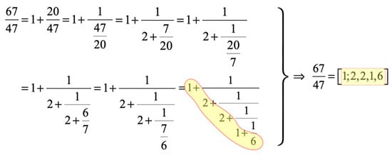
A continued fraction of a rational number a/b is computed as follows: the integer part becomes , leaving the non-negative rational remainder . The latter is now written as , resulting in
Next, the integer part becomes , leaving a rational remainder that is treated as before. This processing stops until the rational remainder is zero. Figure 1 gives an example of the processing.
Figure 1.
Example of a straightforward computation of a continued fraction.
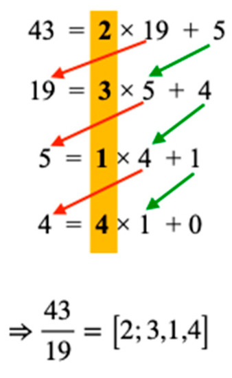
Beside this straightforward proceeding to compute continued fractions, the well-known Euclidian algorithm can be used for this purpose too. Figure 2 gives a corresponding example; it should be self-descriptive.
Figure 2.
Using the Euclidian algorithm to compute a continued fraction.
Formally, a continued fraction can always be reduced such that its last element is greater than or equal to 2.
Note 1.
Let be a continued fraction. Then:
Especially, it can always be achieved that a continued fraction satisfies .
Proof.
The following simple computation proves the first claim:
Furthermore, if in then ≥ 2. This is because, by definition, for 1 ≤ k ≤ N. □
Equation (5) implies a straightforward way to compute the value represented by a continued fraction : see Figure 3.
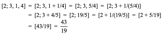
Figure 3.
Computing the value of a continued fraction based on Equation (5).
2.2. Convergents
Next, we define the “workhorses” of the theory of continued fractions.
Definition 2.
is called m-th convergent of the continued fraction for 0 ≤ m ≤ N, or m-th convergent of the infinite regular continued fraction .
Convergents can be computed recursively based on the following theorem:
Theorem 1.
(Recursion Theorem)
Define:
- ;
- ;
- for n ≥ 2;
and define:
- ;
- ;
- for n ≥ 2.
Then, for every convergent
, it is:
Proof (by induction).
Let n = 0, 1: Then, and .
Induction hypothesis: .
Induction step n → n + 1: According to Note 1, it is
and the last continued fraction has n elements, i.e., the induction hypothesis applies:
Here, (A) is valid because of the induction hypothesis, and (B) is the definition of and . □
The recursion theorem implies the often used.
Corollary 1.
Numerators and denominators of convergents of a continued fraction with are strictly monotonically increasing:
Proof (by induction).
Let n = 1: By definition, , . Because for i ≥ 1, and , it is . Similarly,
Now, and for n ≥ 2. With by definition, and (≥1) as well as (≥1) by induction hypothesis, the claim follows. □
The next theorem is about the sign of a combination of the numerators and denominators of consecutive convergents of a continued fraction.
Theorem 2.
(Sign Theorem)
For , the following holds:
Proof (by induction).
For n = 1, it is
Induction step n → n + 1:
(A) uses the induction hypothesis. □
In case the numerators and denominators stem from the n-th convergent and the (n − 2)-nd convergent, the last n-th element of the convergent becomes part of the equation.
Theorem 3.
(Second Sign Theorem)
For , the following holds:
Proof.
It is and .
Multiplying the first equation by and the second equation by results in and . Next, both equations are subtracted:
where (A) is implied by the sign theorem (Theorem 2) and considering . □
The sign theorem immediately yields the important.
Corollary 2.
Numerator and denominator of a convergent are co-prime.
Proof.
Let t be a divisor of and , i.e., and . Then, , but according to the sign theorem. Thus, t = ±1. □
Convergents can be represented as a sum of fractions with alternating sign and whose denominators consist of products of two consecutive denominators from the recursion theorem.
Theorem 4.
(Representation as a Sum)
Each convergent can be represented as a sum:
Proof.
Let . Since , we can write
Computing the differences results in
where the sign theorem is applied in (A) and the last term is the recursion theorem. □
The next theorem is key for many estimations in the domain of continued fractions.
Theorem 5.
(Monotony Theorem)
Let denote the n-th convergent. Then:
and
I.e., even convergents are strictly monotonically increasing, and odd convergents are strictly monotonically decreasing.
Proof.
We compute the following difference, where (A) again uses :
(B) is because of the sign theorem, and (C) follows from , i.e., the recursion theorem.
Now, because of , it is . Thus, for n even and for n odd. This implies for n even as well as for n odd. □
While even convergents are increasing and odd convergence are decreasing, all even convergents are smaller than all odd convergents. This is the content of the next very important theorem.
Theorem 6.
(Convergents Comparison Theorem)
For , it is
Proof.
As before, using the sign theorem in (A), we obtain
with . Because , it is βn > 0, i.e., the sign of is in fact .
Thus, , and we get . This shows that an even convergent is strictly smaller than its immediate succeeding odd convergent .
But what about an arbitrary odd convergent ? For n < m, the monotony theorem (Theorem 6) yields and we showed before that ; thus, .
For n > m, the monotony theorem yields and with we see . □
The following often-used corollary computes the difference of two immediately succeeding convergents by mean of the denominators of the convergents, while the difference of the n-th convergent and the (n − 2)-nd convergent adds the n-th element of the n-th convergent as a factor.
Corollary 3.
and
Proof.
Equation (10) is the first equation from the proof of Theorem 6. The second equation follows because of
where (A) is because of the second sign theorem (Theorem 3). □
We already saw that the even convergents are strictly monotonically increasing, that the odd convergents are strictly monotonically decreasing, and that each even convergent is less than all odd convergents. According to the next theorem, the value of a continued fraction lies between the even convergents and the odd convergents, i.e., this value is larger than all even convergents and smaller than all odd convergents. The situation is depicted in Figure 4.
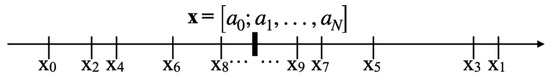
Figure 4.
Nesting of the value of a continued fraction by its convergents.
Note that the notion of the value of a continued fraction is defined for finite continued fractions. In Section 4, this notion will also be defined for regular infinite continued fractions.
Theorem 7.
(Nesting Theorem)
Let x be the value of the continued fraction and let be its convergents. Then:
Proof.
The value of x is the convergent with the highest index N, i.e., .
Let N = 2k be even. Since even convergents are strictly monotonically increasing, we know that , and according to the convergent comparison theorem (Theorem 6), we know .
Let N = 2k + 1 be odd. Since odd convergents are strictly monotonically decreasing, we know that , and according to the convergent comparison theorem (Theorem 6), we know . □
Because the value of a continued fraction is nested within its even convergents and odd convergents, the distance of this value from any of its convergents can be estimated by the distance of two consecutive convergents:
Theorem 8.
(Distance Theorem)
Let and let be its convergents. Then:
and
Proof.
Let n be even. Then, , i.e., . Additionally, it is and . Thus, for n even.
Now, let n be odd. It is , which implies . Because of and , it is ⇔ for n odd.
Together, this proves Equation (13). Equation (14) is proven similarly. □
Figure 5 shows the corresponding geometric situation for an even n.
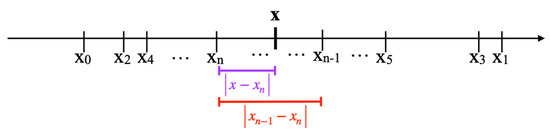
Figure 5.
The distance between two succeeding convergents is greater than the distance of a convergent and the value of its continued fraction.
Similarly, the difference between any two arbitrary convergents can be estimated by the difference of the convergent with the smaller index and its immediate predecessor:
Theorem 9.
(Difference Theorem)
Let and let be its convergents. Then:
Proof.
Let n be even, e.g., n = 2k.
Let m = 2t be even. By Theorem 6, even convergents are smaller than all odd convergents, i.e., for any . Thus, .
Let m = 2t − 1 be odd. By the monotony theorem (Theorem 5), odd convergents are strictly monotonically decreasing, i.e., for each t > k. Thus, .
For n odd, the proof is analogous. □
The geometry of the last theorem is depicted in Figure 6.
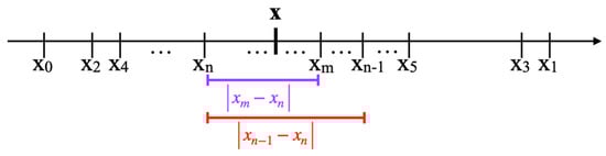
Figure 6.
The distance between any two convergents is smaller than the distance between the convergent with the smaller index and its immediate predecessor.
In several calculations, the size of the denominator of a convergent must be estimated:
Lemma 1.
(Size of Denominators)
For the denominator of a convergent , the following holds:
and
Proof.
By definition, , and because , and finally,
(A) holds because of the recursion theorem (Theorem 1), (B) is by definition of , (C) is because , and (D) has been seen just before (i.e., ). This proves the lemma for .
The proof for n ≥ 3 is by induction. It is
where (A) is the recursion theorem, (B) is because of , (C) is by induction hypothesis applied to , (D) is because n ≥ 3, and (E) is by induction hypothesis applied to . This proves Equation (16).
Equation (17) is proven by induction again. Let n > 3. The argumentation is exactly as before, with the exception of (D):
(D) holds because n > 3, i.e., . □
In fact, denominators of a convergent grow much faster than the inequation may indicate:
Lemma 2.
(Geometric Growth of Denominators)
Let () be the denominator of the convergent . Then:
Proof.
It is , with (A) because, according to corollary 1, denominators are strictly monotonically increasing, i.e., .
By induction, it is , and then with (A) because , and (B) follows from
Similarly, by induction, it is and then with (A) because of .
With and , respectively, Equation (18) is implied. □
2.3. Convergence of Infinite Regular Continuous Fractions
In Section 2.1, we presented an algorithm to compute the continued fraction representation of a rational number. Next, we show how to compute such a representation for a non-rational number (Algorithm 1).
| Algorithm 1 Continued Fraction Representation of Non-Rational Number |
|
The above algorithm does not terminate, i.e., the continued fraction representation of a non-rational number is infinite. This is the content of the following note:
Note 2.
In Algorithm 1, it is .
Proof (by induction).
n = 0: Then, by definition, .
Induction hypothesis: .
n → n + 1: Assume ⇒ ⇒ , which is a contradiction to the hypothesis! Thus, ⇒ . □
Figure 7 gives the computation of the continued fraction representation of :
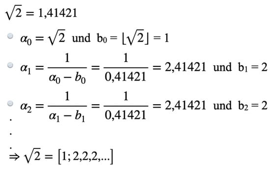
Figure 7.
Computing the continued fraction of .
2.4. Bounds Expressed by Denominators of Convergents
In the following, we give upper bounds and lower bounds of the approximations of a number by the convergents of its continued fraction representation by means of the denominators of the convergents.
First, we start with estimations of upper bounds:
Lemma 3.
(Upper Bounds)
Let be a convergent of the continued fraction representation of x. Then:
Proof.
With , it is (see Theorem 8, Equation (14)). According to Corollary 3 (Equation (10)), it is
Thus,
where (A) holds because of (Corollary 1), and (B) is true because of (Lemma 1). □
An immediate consequence of this theorem is the convergence of the sequence of the convergents of a continued fraction to the value of the continued fraction. This, by the way, is the origin of the name “convergents”.
Corollary 4.
The series of the convergents of the continued fraction representation of converges to x:
Proof.
The claim follows immediately from . □
Often, two fractions are compared by means of their mediant (“mediant” means “somewhere in between”).
Definition 3.
For and b, d > 0, the term is called the mediant of the two fractions.
The following simple inequation is often used.
Note 3.
(Mediant Property)
Let and b, d > 0 and .
Then:
Proof.
It is and . This implies and thus . The inequation follows similarly. □
Mediants of convergents that are weighted in a certain way are another important concept for computing bounds:
Definition 4.
The term with is called the (n,t)-th semiconvergent.
Semiconvergents of an even n are strictly monotonically increasing, and semiconvergents of an odd n are strictly monotonically decreasing. This is the content of the following lemma.
Lemma 4.
(Monotony of Semiconvergents)
Let n be even. Then, .
Let n be odd. Then, .
Proof.
A simple calculation and the use of the sign theorem (Theorem 2) results in
The denominator of the last fraction is always positive. Thus, the last term is positive iff n is even (i.e., ), and it is negative iff n is odd (i.e., ). □
In order to simplify proofs in what follows, the following conventions are used:
With this, becomes a semiconvergent. Now, where (A) is the recursion theorem and (B) follows because ; thus, .
Furthermore, it is for .
Putting things together, it is
Based on this, we can refine Figure 4, which depicts the nesting and ordering of convergents by including semiconvergents: Between two succeeding convergents (e.g., and in Figure 8, the corresponding semiconvergents ordered according to Lemma 4 are nested (in increasing order as shown for an even n in Figure 8). Furthermore, beyond , the semiconvergents are added.
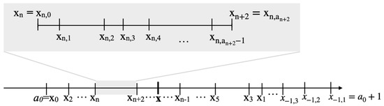
Figure 8.
Nesting of convergents and semiconvergents (n even).
Now, we are prepared to prove a lower bound of the approximation of a number by the convergents of its continued fraction representation by means of the denominators of the convergents.
Lemma 5.
(Lower Bounds)
Let be a convergent of the continued fraction representation of x. Then:
Proof.
The proof is based on the following claims:
Claim 1.
n even ⇒ .
Proof.
is the mediant of and . Thus, the mediant property (Note 3) shows that . Then:
where (A) follows by the monotony of even semiconvergents (Lemma 4), and (B) is the recursion theorem. Because of Theorem 7 (note that n + 2 is even and n + 1 is odd), it is . This proves Claim 1.
Claim 2.
n odd ⇒ .
Proof.
As before, is the mediant of and . Because n is odd, it is (Theorem 7). Thus, because of the mediant property (Note 3). Then:
where (A) follows by the monotony of odd semiconvergents (Lemma 4), and (B) is the recursion theorem. Because of Theorem 7 (note that n − 1 is even and n + 2 is odd), it is , and because n is odd, it is . This proves Claim 2.
With Claim 1, for even n, it is ⇒ .
With Claim 2, for n odd, it is ⇒ ⇔ .
Thus, for any k ∈ ℕ:. Next, we compute
where (A) is the sign theorem (Theorem 2).
This implies . □
Because of (Corollary 1), it is
Using the last inequality in Lemma 5 (Lower Bounds) and using Lemma 3 (Upper Bounds), we obtain the concluding theorem of this section:
In summary, we have proved the following:
Theorem 10.
(Bounds of Approximations by Convergents)
Let be a convergent of the continued fraction representation of x. Then:
□
2.5. Best Approximations
Our goal is to approximate a real number by a rational number as good as possible while keeping the denominator of the rational number “small”. Keeping the denominator small is important because in practice, every real number can only be given up to a certain degree of precision, and this is achieved by means of a huge denominator and corresponding numerator. i.e., approximating a real number by a rational number with a huge denominator is canonical, but finding a small denominator is a problem.
This is captured by the following:
Definition 5.
A fraction is called a best approximation (of the first kind) of :⇔ (assuming c/d ≠ p/q).
Often, the addition “of the first kind” is omitted. By definition, a best approximation of a real number can only be improved if the denominator of the given approximation is increased.
If p/q is a best approximation of α, then is small and, thus, is small. Measuring the goodness of an approximation this way results in the following:
Definition 6.
A fraction is called a best approximation of the second kind of :⇔ (assuming c/d ≠ p/q).
The question is whether every best approximation is also a best approximation of the second kind. Now, 1/3 is a best approximation of 1/5 because the only possible fractions for c/d, with d ≤ 3 = q, are 0, 1/2, 2/3, and 1, and these numbers satisfy .
Next, we observe that with 1 < 3. Thus, with and (i.e., ) and , we found a fraction with ! As a consequence, although 1/3 is a best approximation of the first kind of 1/5, it is not a best approximation of the second kind.
Thus, not all best approximations of the first kind are best approximations of the second kind. But the reverse holds true:
Lemma 6.
(Every 2nd Kind Best Approximation is a 1st Kind Best Approximation)
If is a best approximation of the second kind of , then is also a best approximation of the first kind of α.
Proof (by contradiction).
Assume p/q is not a best approximation of the first kind. Then, for a fraction c/d with d < q. Multiplying both inequations results in ⇔ , which is a contradiction because p/q is a best approximation of the second kind. □
The next simple estimation about the distance of two fractions by means of the product of their denominators is often used.
Note 4.
(Distance of Fractions)
Let with . Then:
Proof.
With and , it is . Also, because otherwise which contradicts the premise. Thus, , i.e., . This implies
where because . □
Next, we prove that every best approximation of the second kind is a convergent.
Theorem 11.
(2nd Kind Best Approximations are Convergents)
Let be a best approximation of the second kind of , and let be the continued fraction representation of x.
Then is a convergent of x.
Proof.
Being a best approximation of the second kind of x, satisfies, by definition, for d ≤ b.
Claim 1.
.
Proof (by contradiction).
Assume ; thus, , where (A) holds because , i.e., 1 ≤ b. This implies , which contradicts for d ≤ b (with and ). This means that , (B) is because of the recursion theorem.
Thus, the geometric situation is as depicted in Figure 9, i.e., is in the grey shaded area being greater than or equal to the convergent . This will be refined in what follows.
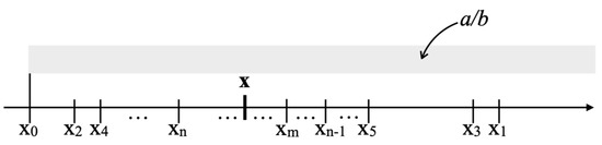
Figure 9.
Any best approximation of the second kind is in the grey shaded area, i.e., greater than or equal to the convergent .
Next, we proceed with a proof by contradiction assuming that is not a convergent of x.
Assumption.
for .
According to Claim 1, . Thus, one of the following must hold:
or
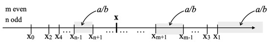
This situation is shown in Figure 10.
Figure 10.
If a best approximation of the second kind is not a convergent, it is within the indicated grey shaded areas.
Case (1).
If (i) is true, then
where (Th8) is Theorem 8, Equation (14), and (C) is from Corollary 3, Equation (10). Furthermore, , with (D) because of Note 4 (Distance of Fractions).
Together, ⇒ ⇒ (iii).
Also, if (i) is true, then , where (E) is again using Note 4. This implies ⇒ (iv).
Lemma 3 (Upper Bounds) tells us that which is equivalent to ⇔ ⇒ (see (iv) just before). Since (see (iii) above), this is a contradiction to being a best approximation of the second kind of x. Thus, Case (1) does not occur.
Case (2).
This case is shown in Figure 11. Then, , where (F) again uses Note 4. This implies (v) with (G) using the recursion theorem.
Figure 11.
Pictorial representation of Case (2).
Now, , where the last inequality holds because of ; thus, , (H) based on (v) before. This means that with , i.e., is not a best approximation of the second kind of x, which is a contradiction. Thus, Case (2) does not occur either.
Consequently, the assumption is wrong and there is a with , i.e., is a convergent. □
So, every best approximation of the second kind is a convergent. The next theorem proves the reverse, i.e., that every convergent is a best approximation of the second kind.
Theorem 12.
(Lagrange, 1798—Convergents are 2nd Kind Best Approximations)
Let be a convergent of , , and . Then, for and it is , i.e., the convergent is a best approximation of the second kind of x.
The cases and are excluded because the convergent is not a best approximation of the second kind of : it is and , which implies . Setting , results in = = . If would be a best approximation of the second kind of x, then > would hold.
The proof of Lagrange’s theorem is very technical. First, the expression is analyzed to find the smallest integral numbers and such that the expression is minimized under the constraint , i.e., is a denominator of a convergent. It is shown both that is a best approximation of the second kind of x, and that and .
Proof.
Let and let be a convergent. First, we are looking for the smallest numbers with such that is minimal.
Step 1.
Pick an arbitrary , and based on this we determine .
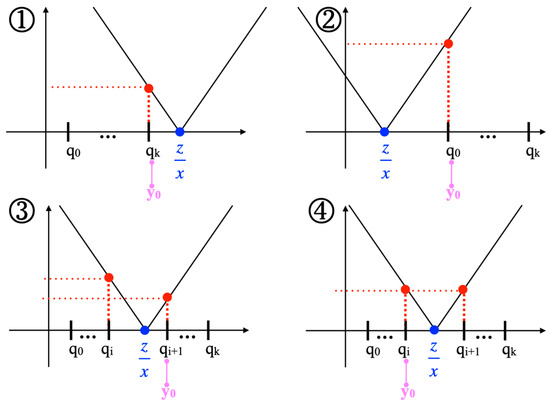
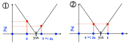
It is , but in general . Looking for a solution that minimizes results in the following potential positions of with respect to the denominators (see Figure 12):
Figure 12.
The potential positions of with respect to the denominators .
- Case 1: . Then, is the solution;
- Case 2: . Then, is the solution;Let for 1 ≤ i ≤ k.
- Case 3: For (i.e., is closer to than to ), is the solution, and for (i.e., is closer to than to ), is the solution;
- Case 4: For (i.e., is exactly in the middle between and ), is the solution because , and we are looking for the smallest , especially .
Step 2.
Based on the found, we determine next. It is , but in general, . In solving the minimization problem within (i.e., ), the following cases can be distinguished (see Figure 13):
Figure 13.
The potential positions of .
- Case 0: It may happen that . Then, choose ;
- Case 1: is between two integral numbers s and t, i.e., . For (i.e., is closer to t than to s), is the solution; and for (i.e., is closer to s than to t), is the solution;
- Case 2: For (i.e., is exactly in the middle between t and s), is the solution because , and we are looking for the smallest .
Claim 1.
is uniquely determined.
Proof (by contradiction).
Assume there exists a with and . This can only happen iff one term is positive and the other is negative, i.e., for example, if and , and then , i.e., .
As an intermediate step we prove:
Claim 2.
and are co-prime, i.e.,
Proof (by contradiction).
Let and with . Then, and thus
Assume . Then, with and , it follows:
Now, has been determined in Step 1 to satisfy for a given z, especially for , i.e., . Because and , it must be . This is a contradiction because according to (ii) before. Thus, , i.e., L = 2.
With and , we get , which implies. By definition of , . However, (see (i) above); thus, , which is a contraction.
We continue the proof of Claim 1: It is and also , i.e., . Because according to Claim 2, it follows that and .
Now, let . Then, it is ((A) uses the recursion theorem (Theorem 1)), and with Note 1, it is . Thus, ((B) is because ). Now:
where (C) holds because of the sign theorem and (D) because (see the end of the proof of Step 1).
Furthermore,
where (E) is true because and, thus, for integral numbers and . Together, we obtained , which is a contradiction to the choice of and ! This proves Claim 1 for .
Now, let and choose (based on Note 1, the highest element of a continued fraction is always greater than or equal 2, thus ). Then
((F) is the recursion theorem) which has been excluded from the theorem.
Thus, let and . Then
where (G) applies the recursion theorem and (H) the sign theorem. Because of (iii), it is , i.e., together, which contradicts the definition of and ! This proves Claim 1 for .
Next, we observe
Claim 3.
is a best approximation of the second kind of x.
Otherwise: for an with , which contradicts the definition of and !
According to Theorem 11, is a convergent of x, i.e., for an . If , the proof is done. Thus, we assume .
Claim 4.
For , it is .
Proof.
⇒ ⇒ (Corollary 1: denominators are monotonically increasing). Similarly, ⇒ ⇒ . Together, this implies .
Next, we get
where (I) is Lemma 5 (Lower Bounds) and (J) is Claim 4.
Furthermore, , where (K) holds because of Lemma 3 (Upper Bounds).
With and the definition of and (i.e., the minimizing property), it is ⇒ , which implies . This is a contradiction; because of the recursion theorem, it is , where (L) holds with . Thus, which proves the overall theorem. □
Putting the last two theorems together yields:
Corollary 5.
is a best approximation of the second kind of x ⇔ x is a convergent of x. □
According to Theorem 12, every convergent is a best approximation of the second kind, and each best approximation of the second kind is also a best approximation of the first kind (Lemma 6). We keep this observation as:
Note 5.
Every convergent is a best approximation of the first kind. □
But are best approximations of the first kind also always convergents? Not quite: the next theorem proves that a best approximation of the first kind is a convergent or a semiconvergent.
Theorem 13.
(Lagrange, 1798—1st Kind Best Approximations are Convergents or Semiconvergents)
Let be a best approximation of the first kind of . Then is a convergent or a semiconvergent of x.
Proof.
By definition, it is for and .
Claim 1.
.
Otherwise: ; thus, . Now, ; thus, ⇒ . Because , we obtained a contradiction since is a best approximation of the first kind.
Claim 2.
.
Otherwise: and based on the geometric situation depicted in Figure 8, it follows that with , which contradicts being a best approximation of the first kind.
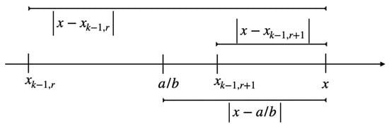
Consequently, lies between and (see Equation (22)), i.e.,
and is, thus, covered by the set of intervals defined by the convergents and semiconvergents of x (see Figure 8).
Assumption.
is neither a convergent nor a semiconvergent.
This results in the following cases:
- Case 1: lies between two semiconvergents and ;
- Case 2: lies between two convergents and ;
- Case 3: lies between a convergent and a semiconvergent.
We will show that all three cases lead to a contradiction, i.e., the assumption must be false; thus, the theorem is proven.
Case 1.
lies between and .
Then,
where (A) results from the same computation performed in the proof of Lemma 4.
Furthermore, it is
where (B) is seen to be valid as follows: and, thus, ; if it would be zero, the first modulus in (i) would be zero, i.e., which contradicts the assumption of the claim, which in turn implies .
Together,
thus,
Because of the monotony of the sequence of semiconvergents (Lemma 4), it is for an odd (i.e., even) (see the geometric situation in Figure 14);
Figure 14.
Distances within an interval of semiconvergents (k odd).
thus,
But with (ii), it is ; thus, is not a best approximation of the first kind to x, which is a contradiction. even leads to a contradiction too, i.e., Case (1) is not possible
Case 2.
lies between and .
Then, where (C) is Equation (11) from Corollary 3, and with Note 4, it is .
Together, ⇒ ⇒ . Because of the geometric situation shown in Figure 15, it is , which is a contradiction to being a best approximation of the first kind to x and .
Figure 15.
Distances within an interval of convergents (k even).
Case 3.
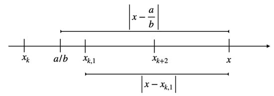
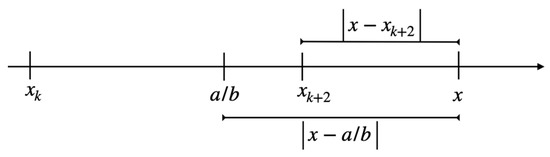
lies between a convergent and a semiconvergent.
This implies that lies between and (see Figure 8), otherwise would lie between two semiconvergents, which has already been covered in Case 1.
Thus, , but
where (D) is the sign theorem. I.e., it is . As before, with Note 4, it is ⇒ ⇒ .
The geometric situation from Figure 16 reveals , which is a contradiction to being a best approximation of the first kind to x and . □
Figure 16.
Situation in which is between a convergent and its first semiconvergent (k even).
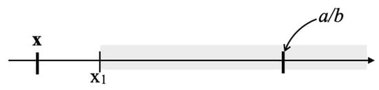
Finally, we give a simple criterion that allows us to prove that a given fraction is a convergent of another real number. This theorem is a cornerstone of computing a prime factor with Shor’s algorithm.
Theorem 14.
(Legendre, 1798—Convergent Criterion)
Let ⇒ is a convergent of x.
Proof.
We show that is a best approximation of the second kind of x. Theorem 11 then proves the claim.
Let for and . We need to prove .
Now, . This implies ⇔ ⇔ . Thus,
With Note 4 (Distance of Fractions), it is also . Together, it is
3. Probability of the Occurrence of Convergents
3.1. Estimating Secant Lengths
In this part, we use the main arguments of [2].
In order to estimate the probability of the occurrence of a certain state after having performed the quantum Fourier transform, we need the following estimation of a lower bound and an upper bound of the length of a secant of the unit circle:
Lemma 7.
(Secant Length Estimation)
If then .
Proof.
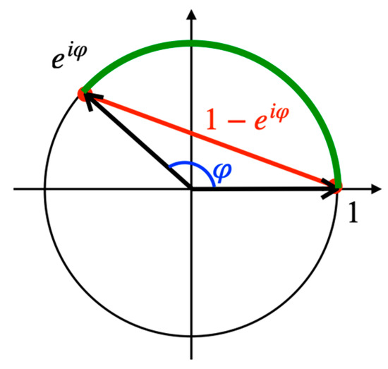
The upper bound follows from elementary geometry, namely that the length of a secant is less than or equal to the length of the corresponding arc of a circle (see Figure 17).
Figure 17.
The length of a secant is smaller than the arc of the corresponding unit circle.
The length of the arc determined by the angle φ on a circle of radius r is , i.e., if the circle is a unit circle, the length of the arc (green in the Figure) is .
A secant of the unit circle (red in the Figure 17) can be defined by the two complex numbers on the unit circle (black in the Figure 17) that are the endpoints of the secant. Thus, the length of this secant is the difference of these complex numbers. One of these points can always be 1 because a corresponding rotation is length-preserving; the other point is then , where is the angle of the arc cut by the secant. The length of this secant is then .
This proves the inequality .
Next, we compute
where (A) uses Euler’s formula, (B) is the definition of the modulus of a complex number with and , (C) is the double-angle formula, and (D) assumes that .
To estimate a lower bound for , we analyze the function . From elementary calculus, it is known that a function is concave on if and only if its second derivative is not positive on D, i.e., on D.
(Reminder: is concave on D:⇔ ,
I.e., for any two points on the graph of , the secant between these points is below the graph, Figure 18).
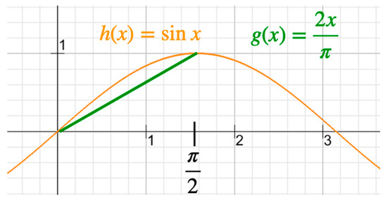
Figure 18.
The graphs of sin x and 2x/π.
With especially for , i.e., is concave on . Thus, the secant between and is below the graph of (orange in Figure 18). However, this secant is given by (green in Figure 18). Thus, it is for , i.e., with we get for , and this implies for .
Now, (see the computation before) implies for .
Furthermore, is convex on ; thus, an argument analogous to the above shows that for . □
3.2. Estimating Amplitude Parameters
As stated in the introduction, the quantum part of Shor’s algorithm produces in its final step the following quantum state via a measurement:
Thus, according to the Born rule, the probability of this particular state |y⟩ is the square of the modulus of the amplitude of |y⟩, i.e.,
The argument of the modulus is a geometric sum with ; thus, in case ,
With . In this section, in order to compute a lower bound for , we investigate some relations between the following parameters appearing in Equation (28):
- n: the number to be factorized;
- N: a power of 2 (e.g., ) with ;
- the choice of N effectively determines the domain of numbers that can be represented in the -part of the quantum register (see Equation (1)).
- p: the period of the modular exponentiation function ;
- A: the number of arguments mapped to a given value of .
We also estimate bounds of the argument of .
3.2.1. Basics from Number Theory
For convenience, we state the definition of the modulo function.
Definition 7.
The modulo function is the following map:
is, thus, the residue left when dividing z by n. I.e., if , then there is a number such that with .
If , we find numbers and such that and with . This implies that , i.e., n is a divisor of (in symbols: ). We also obtain that implies that .
The equation is abbreviated as ; in words, is congruent modulo n. As shown just before, is equivalent to and to . We keep this as
Note 6.
⇔ ⇔ . □
Furthermore, we state the definition of modular exponentiation which turns out to play a key role in finding factors.
Definition 8.
For , the modular exponentiation function is the following map:
The smallest number p that satisfies for all x is called the period of f. Especially, with , we get which means that , i.e., which in turn is equivalent to . Thus, we have proven:
Note 7.
has period p ⇔ ⇔ . □
Finding a factor of n can be achieved by finding the period p of the function . This is seen as follows: Let p be the period of , then , i.e., . Assume p is even (if p is odd, Shor’s algorithm is repeated with a different a, until an even p is found). With such an even p, it is which implies that and have a common divisor, which in turn means that or is a divisor of n. Thus, if an even period has been determined, classically efficient calculations can be used to compute a factor of n. If this factor is a prime number, we can finish. Otherwise, we continue determining a factor of the former factor, and so on, until we end up with a prime factor of n.
Next, we determine an upper bound of the period p of the modular exponentiation by using group theory. A simple calculation shows that “” is an equivalence relation on . The equivalence class of is denoted as and is referred to as the residue class of z modulo n. It is (see Note 6), where the latter set is sometimes written as . The set of all residue classes modulo n is denoted as , i.e., .
We can multiply two residue classes modulo n as follows: . With this multiplication, becomes a group. Because , it is . Since every integer is a divisor of itself, it is (for ), i.e., the cardinality of numbers co-prime to n is less than n: .
The well-known Lagrange’s theorem from group theory states that for a group G with and for each , it is (e is the unit element of G)—see Lemma 3.2.5 in [3], for example. Thus, for , it is , i.e., . Since the period p is the smallest number with , it follows that and, thus, .
Now, the assumption of Shor’s algorithm is that and that , which ensures that ; thus, and .
Lemma 8.
Let p be the period of . Then, . □
3.2.2. Intervals of Consecutive Multiples of the Period
The relation between N and p is depicted in Figure 19; multiples of N are always contained in closed intervals defined by consecutive multiples of p, i.e., it may happen that a multiple of N coincides with a multiple of p.
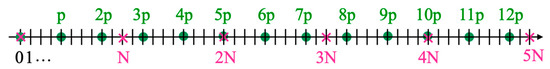
Figure 19.
Multiples of N are enclosed by immediately succeeding multiples of p.
Note 8.
Proof.
Pick an arbitrary , i.e., is also given. Then, we find a such that (trivial because ). Let be the smallest of such , i.e., . Thus, because otherwise , which is a contradiction because t was chosen minimal.
Together, . The claim follows because k an arbitrary number. □
The situation we just discussed is shown in Figure 20.
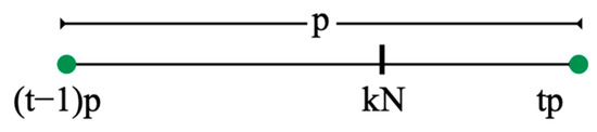
Figure 20.
Determining the interval of succeeding multiples of p enclosing a multiple of N.
Furthermore, two different multiples of N are in different intervals defined by succeeding multiples of p. Otherwise, the situation of Figure 21 would imply that , which is a contradiction as shown by the proof of Note 9 below.
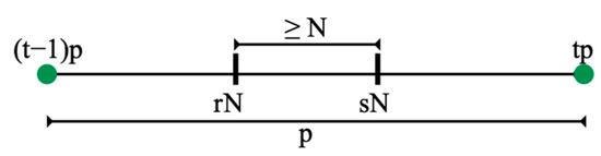
Figure 21.
No two multiples of N can be enclosed by succeeding multiples of p.
We denote a with by . This is justified by the next Note 9 which proves that such a is uniquely determined by . Especially, a multiple is contained in “its” interval:
Note 9.
Let and with .
Then, implies .
Proof (by contradiction).
Assume but with and (see Figure 20). W.l.o.g. ⇒ ⇒ . Further, . Together, it is , i.e., .
According to Lemma 8, we know ⇒ . However, by selection of N (see the bullet list at the beginning of Section 8), it is , which is a contradiction. □
The proof of Note 9 has shown especially:
Corollary 6.
By Note 9, for , the numbers are different, i.e., for each , such a unique exists, i.e., the numbers are different. Thus:
Corollary 7.
There exist p different numbers , , such that . □
These different numbers are strictly monotonically increasing.
Note 10.
Let and with . Then, . Thus, .
Proof (by contradiction).
Assume ; thus, , which implies and .
Now, , , and . This implies and , which finally results in —which is a contradiction to corollary 6 because this would imply that . □
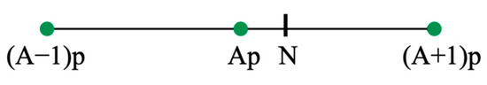
Each multiple of N is “close” to a multiple in the sense that is at most apart from or (see Figure 22).
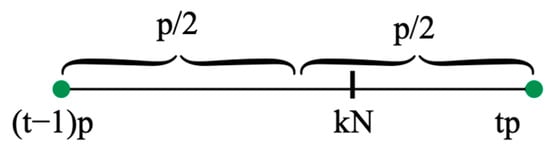
Figure 22.
A multiple of N is always “close” to a multiple of p.
More precisely:
Note 11.
Proof.
It is , i.e., by definition . This implies ∨ (see Figure 22), otherwise:
⇒ , but , i.e., , which is a contradiction! This proves the claim . □
As before, from Note 9, it follows that for , these numbers t are all different. Precisely:
Corollary 8.
Let and such that . If , then . □
The multiples of N are sparsely scattered across the intervals of consecutive multiples of p. More precisely, intervals of consecutive multiples of p, which contain a multiple of N, are not consecutive. This is the content of
Note 12.
Let , , and with .
Then as well as .
Proof.
Because of Note 10, it is ; thus, .
Assumption.
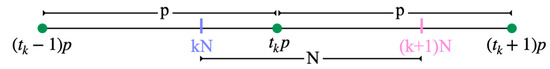
.
By definition, , and by assumption, ; thus, it is . Furthermore, by definition, (see Figure 23).
Figure 23.
Situation in case and lying within two consecutive intervals of consecutive multiples of p.
Now, which implies .
Thus, , i.e., (see Figure 23).
By Lemma 8, it is ⇒ . With ⇒ and by definition of N, it is ; thus, : a contradiction!
Thus, the assumption is false, which implies . The claim is proven similarly. □
The resulting geometric situation is depicted in Figure 24.
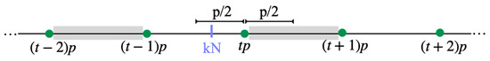
Figure 24.
If is in an interval defined by two consecutive multiples of p, the preceding and succeeding intervals do not contain a multiple of N.
If , it is or (see Figure 22 or Figure 24). In case , we define and results, and in case of , we define implying . According to Note 9, this is uniquely defined. This proves
Note 13.
, i.e., is uniquely determined by . □
This is next rewritten into a format more useful for what follows.
Note 14.
Let and with .
If , then .
Proof.
It is ⇔⇔ ⇔ ⇔ . Note 13 shows that is uniquely determined by . □
Finally, we can prove the following:
Corollary 9.
There exist p different numbers , , such that
Proof.
There exist p different numbers , , such that (Corollary 7). The proof of Note 11 shows that this implies . The proof of Note 14 shows that this implies . □
3.2.3. Cardinality of Pre-Images
First, we show that the parameter A is greater than 1, i.e., at least two numbers available in the -part of the quantum register are mapped by f to the same value.
Note 15.
Proof.
As reminded in the introduction, the quantum Fourier transform of Shor’s algorithm produces the following state:
After measurement of the -part of the register, the -part is in the state
i.e., .
Choose —such an x exists because otherwise it would be , but a period p satisfies . With (Lemma 8) and (by choice of N), it is (see the proof of Note 12). Thus, is in the domain of f (in the sense that it is a value in the -part of the quantum register available as an argument for f), i.e., is available in the -part of the register.
would imply that and, thus, , i.e., for . Since , the function would not be periodic. □
Next, we prove tighter bounds for the parameter A.
Note 16.
Proof.
As in the proof of Note 15, we choose . With
i.e., are all values in the -part of the register being mapped to , i.e., is the largest number satisfying . With , this implies —which is the first part of the claim.
Thus, . Otherwise, and with , it would be , i.e., would also be in the -part of the register being mapped to , which is a contradiction to the definition of A. This proves the second part of the claim. □
The next estimation gives an approximation of in terms of the product of and .
Note 17.
Proof.
Because of , the geometric situation is as depicted in Figure 25, i.e., or . Thus, .
Figure 25.
is embraced by and .
Now, (Lemma 8) and by choice of N. In practice, n is a large number, i.e., is huge compared to n: . Together:
In this sense, is a small number, i.e., is small too: . □
3.2.4. Estimating Arguments of Amplitudes of Potential Measurement Results
The next Lemma is the main result of this section for what follows.
Lemma 9.
Let and . Then:
Proof.
It is ⇔ ⇔ (multiply with p) ⇔ ⇔
By Note 16, it is
Furthermore:
where (A) is because of Note 17 (), and (B) is because of Equation (34) ().
Next, we compute the lower bound for the first fraction of the claim:
where (C) follows from the second inequation of (i) above, (D) is because of , and (E) is implied by (iii) above.
The upper bound for the first fraction of the claim is computed next:
where (F) is implied by the first inequation of (i) above, (G) is (ii) above, (H) follows from the prerequisite , i.e., , and (I) is the first inequation of (ii) above. Finally, we will estimate , and because of , (J) is justified.
Together, , which proves the first claim.
Next,
with (K) from the first inequation of (i) before, (L) because , and (M) because we will estimate . I.e., the upper bound of the second fraction is as claimed.
The correctness of the lower bound is seen as follows:
with the second inequation of (i) before giving (N), (O) is because of , and (Q) is true because ; thus, . □
3.3. Estimating Probabilities
We are now ready to compute the probability that the state |y⟩, which is prepared by the quantum part of Shor’s algorithm, is “close” (i.e., within a distance of ) to a multiple of .
Lemma 10.
Assume and let P be the probability that for a . Then, .
Proof.
According to Equation (29), the probability to measure a particular is
In case (which is the assumption) where (the case will be treated separately in Note 18). Thus, with , it is
The structure of the numerator and denominator recommends the estimation of both by means of the Lemma 7 (Secant Length Estimation). However, applying Lemma 7 requires that . By Lemma 9, we know that under the prerequisite , it is as well as, but Lemma 9 does not imply .
Now, consider the following calculation:
where (A) holds because of , and implies (B): .
Equation (37) allows us to apply the secant length estimation (Lemma 7) because in
it is now according to Lemma 9.
First, we use the second inequation of from Lemma 7 with and obtain
Then, we use the first inequation of from Lemma 7 with and obtain
Using Equations (39) and (40) in Equation (38) results in
This result is now used in Equation (37) (step (C) below) and we obtain
Using Equation (42) in Equation (35) (step (D) below) results in
Thus,
According to Note 17, we know ⇒ , i.e.,
Furthermore, since N is a “huge” number, we know that the following is “small”:
Using Equations (44) and (45) in Equation (43) results in
for each . According to Corollary 9, there exist p different numbers with and for each of them . Since we are not interested in a particular , but in any of them, we need to sum up all probabilities to obtain the overall probability :
This proves the claim. □
We still need to estimate the probability for the case .
Note 18.
Let . Then .
Proof.
In case , the probability is
3.4. Computing the Period
Let y be the result of the measurement produced by Shor’s algorithm. Under the assumption that , the following holds:
Theorem 15.
With probability , there exists a , such that
Proof.
According to Lemma 10, the probability that for a is .
However, ⇔ . Dividing the latter inequations by yields: ⇔.
Thus, . By choice of , it is . Furthermore, ⇒ ⇒ ⇒ . This results in . □
Legendre’s Theorem (Theorem 14) proves immediately:
Theorem 16.
With probability , is a convergent of . □
3.4.1. Determining the Period by Convergents:
The Algorithm 2 determines with probability of approximately the period p we are looking for; is is applicable in the case :
| Algorithm 2 Determining with probability of approximately the period p we are looking for |
|
3.4.2. Determining the Period by Convergents:
In case , the above algorithm is not applicable. However, ⇔ ⇔ ⇔ with . Thus, the Algorithm 3 can be used:
| Algorithm 3 ⇔ ⇔ ⇔ |
|
This may yield the period p but does not guarantee it.
3.5. How the Presented Results Relate
The contribution contains several low-level details. In order to avoid getting lost in these details, this section sketches how the main details contribute to the proof of Shor’s algorithm. The Figure 26 at the end of this section is a cartoon of these relations.
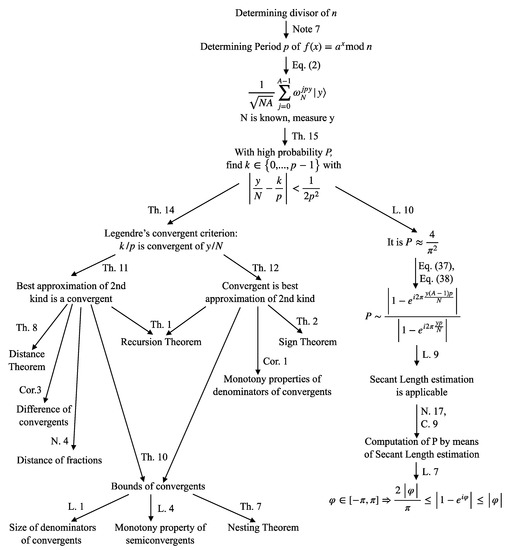
Figure 26.
How the main results of the paper relate.
3.5.1. Applying the Results about Continued Factions
Determining a divisor and finally a prime factor of a natural number can be reduced to finding the period p of the modular exponentiation function for an a with —see Section 3.2.1 and Note 7.
The quantum part of Shor’s algorithm produces the state from Equation (2). Measuring this state results in a natural number .
The natural number N in Equation (2) must be chosen in advance based on the number n to be factorized: it is chosen as with —see the introduction of Section 8. This ensures that the relevant arguments to compute the by the quantum part of Shor’s algorithm can be captured as quantum states.
Theorem 15 guarantees with probability the existence of a such that .
Thus, according to the convergent criterion of Legendre’s Theorem (Theorem 14), is a convergent of .
The proof of Legendre’s convergent criterion (Theorem 14), in turn, is based on the fact that convergents are exactly the best approximations of the second kind (Theorem 11 and Lagrange’s theorem (Theorem 12)).
The proof of Lagrange’s theorem (Theorem 12—each convergent is a best approximation of the second kind) makes use of the recursion theorem (Theorem 1), the sign theorem (Theorem 2), the monotony property of denominators of convergents (Corollary 1), as well as the estimations of the upper bounds of convergents (Lemma 3) and their lower bounds (Lemma 5).
The proof of Theorem 11 (each best approximation of the second kind is a convergent) makes use of the recursion theorem (Theorem 1), the distance theorem (Theorem 8), the computation of the difference of convergents (Corollary 3), the distance of fractions (Note 4), and the estimation of the upper bounds of convergents (Lemma 3).
The estimations of the lower and upper bounds of convergents depend on the distance theorem (Theorem 8), the computation of the difference of convergents (Corollary 3), the monotony property of denominators of convergents (Corollary 1), and on estimations of the size of denominators of convergents (Lemma 1). The estimation of the lower bounds (Lemma 5) makes use of semiconvergents (Definition 4) and their monotony property (Lemma 4) as well as the nesting theorem (Theorem 7).
Remark: Theorem 13, which proves that best approximations of the first kind are convergents or semiconvergents, is not immediately relevant to Shor’s algorithm and may be ignored when focusing on Shor’s algorithm.
3.5.2. Applying Probability Estimations
According to Equation (29) (which is implied by the Born rule), the probability to measure a particular y is for .
Equations (37) and (38) show that this probability can be estimated as . The latter fraction, in turn, can be estimated by means of Lemma 7 (Secant Length Estimation) in case .
Lemma 9 shows that the latter inclusion is satisfied in case of and .
Lemma 10 proves that with probability it is, in fact, for . The proof of this lemma is based on a proper estimation of N (Note 17) which in turn relies on Note 16. Further, it makes use of Corollary 9, which is the summary of the various results of Section 3.2.2.
A simple calculation in the proof of Theorem 15 finally shows that implies . Thus, with probability , the convergent criterion of Legendre’s Theorem (Theorem 14) is satisfied.
4. Conclusions and Related Work
The literature analyzing, discussing, and refining Shor’s algorithm [1] is vast. Of course, most text books on quantaum computing explain the algorithm too (e.g., [4,5]). In doing so, all this literature puts a sharp focus on the quantum part of the algorithm and sketches its classical parts at various depths. However, the mathematical treatment of the classical aspects is sketchy, omitting most of the details and leaving them as an exercise for the reader with references to corresponding text books from mathematics such as [6] or [7]. The lecture notes by Preskill [2] go a bit deeper, especially on the estimation of probabilities, but still omit the low-level details; however, the authors of the contribution at hand benefited a lot by the treatment in [2]. It is noted that the genesis for the authors’ treatment of probability estimations was inspired by unpublished, non-public work to which the authors had access to several years ago.
In doing so, the contribution at hand is very detailed on the probability estimation of being able to use Legendre’s Theorem in Shor’s algorithm. The authors are not aware of any other publication providing these low-level details.
Furthermore, the contribution at hand is a self-contained treatment on continued fractions up to Legendre’s Theorem. All background that is needed to understand this theorem is presented, including all proofs with low-level details step by step.
The authors hope to foster the comprehension of the classical aspects of Shor’s algorithm even at the level of beginners in quantum computing.
Author Contributions
Writing—original draft, F.L.; Writing—review & editing, J.B. All authors have read and agreed to the published version of the manuscript.
Funding
This work was partially funded by the BMWK project PlanQK (01MK20005N).
Institutional Review Board Statement
Not applicable.
Informed Consent Statement
Not applicable.
Data Availability Statement
Not applicable.
Conflicts of Interest
The authors declare no conflict of interest.
References
- Shor, P.W. Polynomial-Time Algorithms for Prime Factorization and Discrete Logarithms on a Quantum Computer. SIAM J. Sci. Stat. Comput. 1997, 26, 1484–1509. [Google Scholar] [CrossRef] [Green Version]
- Preskill, J. Lecture on Quantum Information—Chapter 6. Quantum Algorithms; California Institute of Technology: Pasadena, CA, USA, 2020; Available online: http://theory.caltech.edu/~preskill/ph219/chap6_20_6A.pdf (accessed on 11 July 2022).
- Shult, E.; Surowski, D. Algebra; Springer: Berlin/Heidelberg, Germany, 2015. [Google Scholar]
- Nielsen, M.A.; Chuang, I.L. Quantum Computation and Quantum Information; Cambridge University Press: Cambridge, UK, 2016. [Google Scholar]
- Rieffel, E.; Polak, W. Quantum Computing: A Gentle Introduction; The MIT Press: Cambridge, MA, USA, 2011. [Google Scholar]
- Hardy, G.H.; Wright, E.M. An Introduction to the Theory of Numbers, 4th ed.; Oxford University Press: New York, NY, USA, 1975. [Google Scholar]
- Khinchin, A.Y. Continued Fractions, 3rd ed.; The University of Chicago Press: Chicago, IL, USA, 1964. [Google Scholar]
Publisher’s Note: MDPI stays neutral with regard to jurisdictional claims in published maps and institutional affiliations. |
© 2022 by the authors. Licensee MDPI, Basel, Switzerland. This article is an open access article distributed under the terms and conditions of the Creative Commons Attribution (CC BY) license (https://creativecommons.org/licenses/by/4.0/).