On the Exact Solution of Nonlocal Euler–Bernoulli Beam Equations via a Direct Approach for Volterra-Fredholm Integro-Differential Equations

Abstract

First, we develop a direct operator method for solving boundary value problems for a class of nth order linear Volterra–Fredholm integro-differential equations of convolution type. The proposed technique is based on the assumption that the Volterra integro-differential operator is bijective and its inverse is known in closed form. Existence and uniqueness criteria are established and the exact solution is derived. We then apply this method to construct the closed form solution of the fourth order equilibrium equations for the bending of Euler–Bernoulli beams in the context of Eringen’s nonlocal theory of elasticity (two phase integral model) under a transverse distributed load and simply supported boundary conditions. An easy to use algorithm for obtaining the exact solution in a symbolic algebra system is also given.

1. Introduction

The classical (local) theory of elasticity can adequately describe the behavior of beams, plates, shells and other structures under several loading cases and boundary constraints in almost all engineering applications. However, it has been proved insufficient when used to model newer materials with inherent microstructure, where internal material characteristic lengths become comparable to external characteristic lengths, as in the cases of geometric singularities and micro and nano-scale structural elements [1,2]. This is mainly attributed to the absence of a characteristic scale parameter in the constitutive equations. In contrast, higher order continuum theories such us the Cosserat theory [3], the couple stress theory [4], the micropolar theory [5] and the strain gradient theory [6,7] seem to be appropriate in these cases. These theories incorporate additional material parameters in the constitutive equations and are mathematically more complex and, therefore, numerical methods, especially the finite element method, are employed to solve the governing equations [8,9,10,11]. Alternatively, nonlocal theories such as the nonlocal theory for linear elasticity of Eringen [12] can be used.

In nonlocal elasticity, the stress at a reference point is thought to depend not only on the strain at that point, as in classical theory (‘local model’), but on the strain at every point in the body. In Eringen’s nonlocal theory, this constitutive relationship is realized through an integrated average of the strain field regulated by a kernel called the attenuation function. This formalism of Eringen’s nonlocal elasticity is known as the ‘nonlocal integral model’ [12]. By taking a suitable modified attenuation function, the nonlocal integral model can be converted to a variant that has the sum of both local and nonlocal integral models whose weights are controlled by two parameters. This type of constitutive equation is called the ‘two phase nonlocal integral model’ [13,14,15]. The first nonlocal constitutive model leads to integral equations of equilibrium while the second to integro-differential equations. Recognizing the difficulties associated with solving those integral equations, Eringen proposed a simplified version of the nonlocal constitutive equations in differential form, referred to as the ‘nonlocal differential model’, which provides easy-to-use differential equilibrium equations [12]. Because of its simplicity, the nonlocal differential model has widely been used to analyze various nanoscale structures including one-dimensional nanostructures such as rods, tubes and beams, see the two review papers [16,17], in [18] and others as the literature on the subject is vast.

In particular, for the beam bending analysis, the interested reader can look at, among others, [19,20,21,22,23]. However, several authors have reported that the differential formulation of Eringen’s nonlocal beam theory for specific types of loading gives inconsistent results compared to those obtained from other types of load and boundary conditions [19,24]. This paradox has recently been explained in [25], where it is shown that, in general, the nonlocal differential model is not equivalent to its integral counterpart, unless certain conditions are met as defined in [26]. As a result, there is a great need for further study of the nonlocal integral models despite the relative difficulties.

Closed form solutions of Eringen’s nonlocal integral model for the bending of Euler–Bernoulli beams have been obtained in [27], where the Fredholm type integral governing equations are converted to Volterra integral equations which are then solved by Laplace transform methods. Analytical solutions for the static bending analysis of Euler–Bernoulli beams using Eringen’s two phase nonlocal integral model have been obtained in [28] through a reduction method. Specifically, the governing fourth order integro-differential equation in terms of the transverse displacement (deflection) after integrating twice and substituting the second derivative of the displacement by another function is converted into a linear integral equation of the second kind, which is then reduced to a second order differential equation with mixed boundary conditions as proposed by [26]. After the exact solution of the differential equation and following the reverse path, the analytical solution of the initial governing equation is obtained. A finite element formulation for the two phase nonlocal integral model is presented in [29].

In general, integro-differential equations are usually difficult to solve directly, and therefore, several techniques have been suggested for their reduction to integral or differential equations that are easier to solve [26], while at the same time numerous numerical methods have been developed [30,31,32,33,34,35,36]. Many different numerical methods are used to solve the Volterra–Fredholm integro-differential equations (VFIDE), see for example the series solution methods, variational iteration methods and decomposition methods [37], collocation methods [38,39], Galerkin methods [40], quadrature methods [41], fixed point methods [42] and others. The author and his co-workers in [43] proposed a direct operator technique for solving exactly Fredholm integro-differential equations (FIDE) of the second kind and later advanced it to the solution of nonlinear FIDE [44] and boundary value problems for FIDE and systems of FIDE with nonlocal boundary conditions [45]. The method assumes that the corresponding differential operator is bijective and its inverse is explicitly known.

Motivated by these developments, this work primarily aims at extending the solution procedure in [43,44,45] to solving in closed form boundary value problems for a class of nth order linear Volterra–Fredholm integro-differential equations (VFIDE) of convolution type. Second, to apply this method to construct the closed form solution of the fourth order equilibrium equation for the bending of Euler–Bernoulli beams in the context of Eringen’s two phase nonlocal integral theory of elasticity. This is accomplished via the factorization of the fourth order integro-differential equation into a second order differential equation (DE) and a second order VFIDE.

For this, we consider the VFIDE of convolution type of the general form

$$\begin{array}{ccc}\hfill \sum _{i=0}^n{a}_i{u}^{(n-i)}\left(x\right)& +& \sum _{i=0}^n{\int }_0^x{k}_i(x-t)u^{(n-i)}\left(t\right)dt\hfill \\ & -& \sum _{j=1}^m{\int }_0^L{\overline{k}}_j(x,t)\sum _{i=0}^n{a}_i{u}^{(n-i)}\left(t\right)dt=f\left(x\right),\hfill \end{array}$$

(1)

subject to the boundary conditions

$${\mathsf{\Phi }}_i\left(u\right)=0,i=1,2,\dots ,n,$$

(2)

where $a_i,i=0,1,\dots ,n,$ are real constants with $a_0\ne 0$, $u\left(x\right)$ is n times continuously differentiable function, $u^{\left(i\right)}\left(x\right)=\frac{d^{i}u}{d{x}^i}$, the kernels $k_i(x-t),i=0,1,\dots ,n,$ and ${\overline{k}}_j(x,t),j=1,2,\dots ,m$ are continuous functions, the input function $f\left(x\right)$ is taken to be continuous, $L>0$ and ${\mathsf{\Phi }}_i,i=1,2,\dots ,n,$ are linear continuous functionals. We provide a ready to use symbolic formula for computing the exact solution of (1), (2) in the case where the associated Volterra integro-differential operator is bijective and its inverse is known in closed form and the kernels ${\overline{k}}_j(x,t)$ are separable, i.e.,

$${\overline{k}}_j(x,t)=g_j\left(x\right)h_j\left(t\right),j=1,2,\dots ,m.$$

(3)

The proposed method is used to derive the closed form solution of the two phase nonlocal integral model of Euler–Bernoulli elastic beams in the case of simply supported boundary conditions and under any transverse distributed load that meets the necessary continuity requirements.

The outline of the paper is as follows. In Section 2, the direct operator method for solving boundary value problems for VFIDE is presented. In Section 3, the nonlocal Euler–Bernoulli equations are explained. The decomposition of these equations into a second order DE and a second order VFIDE and their solutions are developed in Section 4. In Section 5, two problems are solved and the results are discussed. In the last Section 6, some conclusions are drawn.

2. Operator Method for Solving VFIDE

Let $X=C[0,L]$, $L\in {\mathbb{R}}^{+}$, and $A:X\to X$ be an nth order linear differential operator of the form

$$Au=\sum _{i=0}^n{a}_i{u}^{(n-i)}\left(x\right),\mathcal{D}\left(A\right)=\{u\in X_n:\mathsf{\Phi }\left(u\right)=\mathbf{0}\},$$

(4)

where $n\in \mathbb{N}$, $a_i,i=0,1,\dots ,n,$ are real constants with $a_0\ne 0$, $u=u\left(x\right)\in X_n=C^n[0,L]$, $u^{\left(i\right)}\left(x\right)=\frac{d^{i}u}{d{x}^i},i=1,2,\dots ,n,$ and

$$\mathsf{\Phi }\left(u\right)=\left(\begin{array}{c}{\mathsf{\Phi }}_1\left(u\right)\\ {\mathsf{\Phi }}_2\left(u\right)\\ ⋮\\ {\mathsf{\Phi }}_n\left(u\right)\end{array}\right)=\mathbf{0},$$

(5)

where ${\mathsf{\Phi }}_i\in X_{n-1}^{*},i=1,2,\dots ,n,$ are linear bounded functionals that describe the specified boundary conditions, $\mathsf{\Phi }\in {\left[X_{n-1}^{*}\right]}^n$, and $\mathbf{0}$ denotes the zero column vector. Let $K:X\to X$ be the linear Volterra integral operator of convolution type

$$Ku=\sum _{i=0}^n{\int }_0^x{k}_i(x-t)u^{(n-i)}\left(t\right)dt,$$

(6)

where the kernels $k_i\left(x\right)\in X,i=0,1,\dots ,n$. Let the row and column vectors, respectively,

$$\begin{array}{ccc}\hfill g& =& \left(\begin{array}{cccc}{g}_1& g_2& \cdots & g_m\end{array}\right),\hfill \\ \hfill \mathsf{\Psi }\left(v\right)& =& \left(\begin{array}{c}{\mathsf{\Psi }}_1\left(v\right)\\ {\mathsf{\Psi }}_2\left(v\right)\\ ⋮\\ {\mathsf{\Psi }}_m\left(v\right)\end{array}\right),{\mathsf{\Psi }}_j\left(v\right)={\int }_0^L{h}_j\left(t\right)v\left(t\right)dt,j=1,2,\dots ,m,\hfill \end{array}$$

(7)

where the functions $g_j=g_j\left(x\right)$ and $h_j\left(t\right)\in X,j=1,2,\cdots ,m,$$g\in X^m$, the function $v\in X$, and ${\mathsf{\Psi }}_j\in X^{*},j=1,2,\dots ,m,$ are linear integral (Fredholm type) functionals with limits from 0 to L and $\mathsf{\Psi }\in {\left[X^{*}\right]}^m$.

Consider the linear Volterra–Fredholm integro-differential operator $T:X\to X$ defined by

$$\begin{array}{ccc}\hfill Tu& =& Au+Ku-g\mathsf{\Psi }\left(Au\right),\hfill \\ \hfill \mathcal{D}\left(T\right)& =& \mathcal{D}\left(A\right)=\{u\in X_n:\mathsf{\Phi }\left(u\right)=\mathbf{0}\},\hfill \end{array}$$

(8)

and write the boundary value problem (1), (2) and (3) in the symbolic form

$$\begin{array}{c}\hfill Tu=f,f=f\left(x\right)\in X.\end{array}$$

(9)

For the solution of problem (9), we prove Theorem 1 below, but first we explain some relations which will use. By $\mathsf{\Psi }\left(g\right)$ we symbolize the $m\times m$ matrix

$$\mathsf{\Psi }\left(g\right)=\left(\begin{array}{cccc}{\mathsf{\Psi }}_1\left(g_1\right)& {\mathsf{\Psi }}_1\left(g_2\right)& \cdots & {\mathsf{\Psi }}_1\left(g_m\right)\\ {\mathsf{\Psi }}_2\left(g_1\right)& {\mathsf{\Psi }}_2\left(g_2\right)& \cdots & {\mathsf{\Psi }}_2\left(g_m\right)\\ ⋮& ⋮& \ddots & ⋮\\ {\mathsf{\Psi }}_m\left(g_1\right)& {\mathsf{\Psi }}_m\left(g_2\right)& \cdots & {\mathsf{\Psi }}_m\left(g_m\right)\end{array}\right),$$

where the element ${\mathsf{\Psi }}_i\left(g_j\right)$ is the value of the functional ${\mathsf{\Psi }}_i$ on the element $g_j$. It is easy to show that for a $m\times k$ constant matrix C,

$$\mathsf{\Psi }\left(gC\right)=\mathsf{\Psi }\left(g\right)C.$$

(10)

The notation $I_m$ indicates the $m\times m$ identity matrix.

Theorem 1.

Let the operator $T:X\to X$ be defined as in (8). Assume that the Volterra integro-differential operator $D:X\to X$ defined by

$$Du=(A+K)u,\mathcal{D}\left(D\right)=\mathcal{D}\left(A\right),$$

(11)

is bijective on X and its inverse is denoted by $D^{-1}={(A+K)}^{-1}$. Then the operator T is bijective, precisely it is injective if and only if

$$detW=det\left[I_m-\mathsf{\Psi }\left(A{D}^{-1}g\right)\right]\ne 0,$$

(12)

and in this case the unique solution to the boundary value problem

$$Tu=f,forallfunctionsf\in X,$$

(13)

is given by the formula

$$\begin{array}{ccc}\hfill u& =& T^{-1}f\hfill \\ & =& D^{-1}f+D^{-1}g{W}^{-1}\mathsf{\Psi }\left(A{D}^{-1}f\right).\hfill \end{array}$$

(14)

Proof. 

Suppose $detW\ne 0$ and $u\in kerT$. Then

$$Tu=Au+Ku-g\mathsf{\Psi }\left(Au\right)=Du-g\mathsf{\Psi }\left(Au\right)=0,$$

and since the operator $D=A+K$ is bijective, we have

$$u=D^{-1}g\mathsf{\Psi }\left(Au\right).$$

(15)

Acting by the operator A on both sides of (15) and then by the vector $\mathsf{\Psi }$, we obtain successively

$$\begin{array}{ccc}\hfill Au& =& A{D}^{-1}g\mathsf{\Psi }\left(Au\right),\hfill \\ \hfill \mathsf{\Psi }\left(Au\right)& =& \mathsf{\Psi }\left(A{D}^{-1}g\mathsf{\Psi }\left(Au\right)\right)=\mathsf{\Psi }\left(A{D}^{-1}g\right)\mathsf{\Psi }\left(Au\right),\hfill \end{array}$$

(16)

by means of (10), from where it is implied that

$$\left[I_m-\mathsf{\Psi }\left(A{D}^{-1}g\right)\right]\mathsf{\Psi }\left(Au\right)=W\mathsf{\Psi }\left(Au\right)=\mathbf{0}.$$

This, under the hypothesis, means that $\mathsf{\Psi }\left(Au\right)=\mathbf{0}$ and as a consequence it follows from (15) that $u=0$, i.e., $kerT=\left\{0\right\}$ and hence the operator T is injective. Conversely, we assume that T is injective and we will prove that $detW\ne 0$ or equivalently, we suppose $detW=0$ and we will show that T is not injective. Then, there exists a nonzero vector of constants $\mathbf{c}=\mathrm{col}(c_1,\dots ,c_m)$ such that $W\mathbf{c}=\mathbf{0}$. Consider the element $u_0=D^{-1}g\mathbf{c}$ and notice that $u_0\ne 0$; otherwise

$$W\mathbf{c}=\left[I_m-\mathsf{\Psi }\left(A{D}^{-1}g\right)\right]\mathbf{c}=\mathbf{c}-\mathsf{\Psi }\left(A{D}^{-1}g\right)\mathbf{c}=\mathbf{c}-\mathsf{\Psi }\left(A{D}^{-1}g\mathbf{c}\right)=\mathbf{c}=\mathbf{0},$$

which contradicts the assumption that $\mathbf{c}$ is nonzero. Since $D=A+K$ is bijective and $\mathcal{D}\left(D\right)=\mathcal{D}\left(A\right)$ it is implied that $u_0=D^{-1}g\mathbf{c}\in \mathcal{D}\left(A\right)$ and hence

$$\begin{array}{ccc}\hfill T{u}_0& =& D{u}_0-g\mathsf{\Psi }\left(A{u}_0\right)\hfill \\ & =& g\mathbf{c}-g\mathsf{\Psi }\left(A{D}^{-1}g\mathbf{c}\right)\hfill \\ & =& g\mathbf{c}-g\mathsf{\Psi }\left(A{D}^{-1}g\right)\mathbf{c}\hfill \\ & =& g\left[I_m-\mathsf{\Psi }\left(A{D}^{-1}g\right)\right]\mathbf{c}\hfill \\ & =& gW\mathbf{c}=\mathbf{0}.\hfill \end{array}$$

This means that $u_0\in kerT$ and so T is not injective.

Suppose now the condition (12) holds true and consider the boundary value problem in (13), namely

$$\begin{array}{ccc}\hfill Tu& =& Au+Ku-g\mathsf{\Psi }\left(Au\right)=Du-g\mathsf{\Psi }\left(Au\right)=f,f\in X,\hfill \\ \hfill \mathcal{D}\left(T\right)& =& \mathcal{D}\left(A\right).\hfill \end{array}$$

(17)

Since by hypothesis the operator $D=A+K$ is bijective, we obtain

$$u=D^{-1}f+D^{-1}g\mathsf{\Psi }\left(Au\right).$$

(18)

Acting as before by the operator A and the vector $\mathsf{\Psi }$ on (18), we have

$$\begin{array}{ccc}\hfill Au& =& A{D}^{-1}f+A{D}^{-1}g\mathsf{\Psi }\left(Au\right),\hfill \\ \hfill \mathsf{\Psi }\left(Au\right)& =& \mathsf{\Psi }\left(A{D}^{-1}f\right)+\mathsf{\Psi }\left(A{D}^{-1}g\right)\mathsf{\Psi }\left(Au\right),\hfill \end{array}$$

from where it follows that

$$\mathsf{\Psi }\left(Au\right)={\left[I_m-\mathsf{\Psi }\left(A{D}^{-1}g\right)\right]}^{-1}\mathsf{\Psi }\left(A{D}^{-1}f\right).$$

(19)

Substitution of (19) into (18) yields

$$u=D^{-1}f+D^{-1}g{\left[I_m-\mathsf{\Psi }\left(A{D}^{-1}g\right)\right]}^{-1}\mathsf{\Psi }\left(A{D}^{-1}f\right),$$

(20)

which is the solution of the boundary value problem (17) or (13).

Finally, notice that the solution (20) holds for any $f\in X$. Consequently, $\mathcal{R}\left(T\right)=X$ and so the operator T is bijective.    □

3. The Two Phase Nonlocal Integral Euler–Bernoulli Beam Model

With reference to a Cartesian coordinate system, with origin O and axis lines $x,y$ and z, consider a uniform beam of length L and cross-sectional area S, whose longitudinal axis coincides with the x-axis, with the one end at $x=0$ and the other end at $x=L$, and its thickness (height) is taken along the z-axis. Let $w\left(x\right)$ be the displacement in z-direction when the beam deforms due to an applied transverse distributed load $q\left(x\right)$ at the top. The equations that model the static bending behavior of Euler–Bernoulli beams in the two phase nonlocal integral formulation of Eringen’s theory of elasticity are as follows.

From [28], we recall that the strain in the x-direction is defined by

$${\epsilon }_x\left(x\right)=-z\frac{d^{2}w\left(x\right)}{d{x}^2}.$$

For a linear homogeneous and isotropic material, the associated nonlocal stress ${\sigma }_x\left(x\right)$ is a expressed as

$${\sigma }_x\left(x\right)=E\left({\xi }_1{\epsilon }_x\left(x\right)+{\xi }_2{\int }_0^{L}k(x,t){\epsilon }_x\left(t\right)dt\right),$$

and the corresponding bending moment is defined by

$$M\left(x\right)={\int }_S^{}{\sigma }_x\left(x\right)zdS=-EI\left({\xi }_1\frac{d^{2}w\left(x\right)}{d{x}^2}+{\xi }_2{\int }_0^{L}k(x,t)\frac{d^{2}w\left(t\right)}{d{t}^2}dt\right),$$

(21)

where E is the elasticity modulus (constant) and $I={\int }_S^{}{z}^{2}dS$ is the second moment of area. The parameters ${\xi }_1>0$, ${\xi }_2>0$ and ${\xi }_1+{\xi }_2=1$ regulate the contribution from the local (classical) and nonlocal model, respectively. The kernel or attenuation function $k(x,t)$ determines the nonlocal effect of the strain ${\epsilon }_x\left(t\right)$ at the source point t on the stress ${\sigma }_x\left(x\right)$ at the receiver point x, and it is usually taken to be of the Helmholtz form

$$k(x,t)=\frac{1}{2\tau }{e}^{-\frac{|x-t|}{\tau }},x,t\in [0,L].$$

(22)

The parameter $\tau =\frac{e_{0}a}{\ell }$, where $e_0$ is a constant related to each material, a is an internal characteristic length (e.g., lattice parameter, granular distance) and ℓ is an external characteristic length (e.g., the crack length, the wave length). The kernel $k(x,t)$ is a positive function which diminishes rapidly as $|x-t|$ increases and satisfies the normalizing condition ${\int }_0^{L}k(x,t)dt=1$.

The principle of virtual displacements requires

$$-{\int }_0^{L}M\left(x\right)\frac{d^2\delta w\left(x\right)}{d{x}^2}dx-{\int }_0^{L}q\left(x\right)\delta w\left(x\right)dx=0,$$

from where after integrating twice by parts, we obtain the Euler-Lagrange or equilibrium equation

$$\frac{d^{2}M\left(x\right)}{d{x}^2}+q\left(x\right)=0,0<x<L,$$

which by means of the definition (21) may be expressed in terms of the displacement $w\left(x\right)$ as

$$-EI\frac{d^2}{d{x}^2}\left({\xi }_1\frac{d^{2}w\left(x\right)}{d{x}^2}+{\xi }_2{\int }_0^{L}k(x,t)\frac{d^{2}w\left(t\right)}{d{t}^2}dt\right)+q\left(x\right)=0,0<x<L,$$

(23)

and the boundary conditions

$$w\left(x\right)\mathrm{or}{M}^{\prime }\left(x\right),$$

and

$$w^{\prime }\left(x\right)\mathrm{or}M\left(x\right),$$

specified at each of the two ends of the beam at $x=0$ and $x=L$.

For a beam simply supported at both ends, the boundary conditions imposed at $x=0$ and $x=L$ are

$$w\left(0\right)=w\left(L\right)=0,M\left(0\right)=M\left(L\right)=0,$$

(24)

or by means of (21),

$$\begin{array}{ccc}\hfill w\left(0\right)=w\left(L\right)& =& 0,\hfill \\ \hfill -EI\left[{\xi }_1{\left(\frac{d^{2}w\left(x\right)}{d{x}^2}\right)}_{x=0}+{\xi }_2{\int }_0^{L}k(0,t)\frac{d^{2}w\left(t\right)}{d{t}^2}dt\right]& =& 0,\hfill \\ \hfill -EI\left[{\xi }_1{\left(\frac{d^{2}w\left(x\right)}{d{x}^2}\right)}_{x=L}+{\xi }_2{\int }_0^{L}k(L,t)\frac{d^{2}w\left(t\right)}{d{t}^2}dt\right]& =& 0.\hfill \end{array}$$

(25)

4. Formulation and Solution of the Problem

To find the solution of the fourth order integro-differential Equation (23) subject to nonlocal boundary conditions (25), we first formulate the problem in an operator form and then decompose it into two lower order problems, specifically, a second order differential boundary value problem and a second order Fredholm integro-differential boundary value problem.

Let $X=C[0,L]$ and the operator $B:X\to X$ be defined by

$$\begin{array}{ccc}\hfill Bw\left(x\right)& =& \frac{d^2}{d{x}^2}\left(\frac{d^{2}w\left(x\right)}{d{x}^2}+\frac{{\xi }_2}{{\xi }_1}{\int }_0^{L}k(x,t)\frac{d^{2}w\left(t\right)}{d{t}^2}dt\right),\hfill \\ \hfill \mathcal{D}\left(B\right)& =& \left\{w\left(x\right)\in C^4[0,L]:w\left(0\right)=w\left(L\right)=0,\right.\hfill \\ & & {\left(\frac{d^{2}w\left(x\right)}{d{x}^2}\right)}_{x=0}+\frac{{\xi }_2}{{\xi }_1}{\int }_0^{L}k(0,t)\frac{d^{2}w\left(t\right)}{d{t}^2}dt=0,\hfill \\ & & \left.{\left(\frac{d^{2}w\left(x\right)}{d{x}^2}\right)}_{x=L}+\frac{{\xi }_2}{{\xi }_1}{\int }_0^{L}k(L,t)\frac{d^{2}w\left(t\right)}{d{t}^2}dt=0\right\}.\hfill \end{array}$$

(26)

Then, the boundary value problem (23), (25) is written compactly as

$$Bw\left(x\right)=\frac{1}{EI{\xi }_1}q\left(x\right),0<x<L.$$

(27)

The operator B can be decomposed as follows. Let the second order linear Fredholm integro-differential operator of the second kind $B_2:X\to X$ be defined by

$$\begin{array}{ccc}\hfill B_{2}w\left(x\right)& =& \frac{d^{2}w\left(x\right)}{d{x}^2}+\frac{{\xi }_2}{{\xi }_1}{\int }_0^{L}k(x,t)\frac{d^{2}w\left(t\right)}{d{t}^2}dt,\hfill \\ \hfill \mathcal{D}\left(B_2\right)& =& \left\{w\left(x\right)\in C^2[0,L]:w\left(0\right)=w\left(L\right)=0\right\},\hfill \end{array}$$

(28)

and the second order linear differential operator $B_1:X\to X$ by

$$\begin{array}{ccc}\hfill B_{1}y\left(x\right)& =& \frac{d^{2}y\left(x\right)}{d{x}^2},\hfill \\ \hfill \mathcal{D}\left(B_1\right)& =& \left\{y\left(x\right)\in C^2[0,L]:y\left(0\right)=y\left(L\right)=0\right\},\hfill \end{array}$$

(29)

where $B_{2}w\left(x\right)=y\left(x\right)$. Then the operator B by means of (28) and (29) can be written as the composition

$$Bw\left(x\right)=B_1{B}_{2}w\left(x\right),$$

and thus the boundary value problem (27) degenerates to

$$B_1{B}_{2}w\left(x\right)=\frac{1}{EI{\xi }_1}q\left(x\right),0<x<L.$$

(30)

The solution of (30) can be found by solving in succession the following differential boundary value problem (DBVP) and Fredholm integro-differential boundary value problem (FIDBVP), respectively:

$$\begin{array}{ccc}\hfill \mathrm{DBVP}:B_{1}y\left(x\right)& =& \frac{1}{EI{\xi }_1}q\left(x\right),0<x<L,\hfill \end{array}$$

(31)

$$\begin{array}{ccc}\hfill \mathrm{FIDBVP}:B_{2}w\left(x\right)& =& y\left(x\right),0<x<L.\hfill \end{array}$$

(32)

4.1. Solution of DBVP

The solution of the linear differential boundary value problem (31) can be constructed easily. It is known that the differential operator $B_1$ defined in (29) is invertable and that its inverse for any function $r\left(x\right)\in X$ is

$$B_1^{-1}r\left(x\right)={\int }_0^x(x-t)r\left(t\right)dt-\frac{x}{L}{\int }_0^L(L-t)r\left(t\right)dt,$$

(33)

see, for example, in [46]. Thus, the solution to boundary value problem (31) in closed form is given by

$$\begin{array}{ccc}\hfill y\left(x\right)& =& B_1^{-1}\left(\frac{1}{EI{\xi }_1}q\left(x\right)\right)\hfill \\ & =& \frac{1}{EI{\xi }_1}\left({\int }_0^x(x-t)q\left(t\right)dt-\frac{x}{L}{\int }_0^L(L-t)q\left(t\right)dt\right).\hfill \end{array}$$

(34)

4.2. Solution of FIDBVP

Substituting $y\left(x\right)$ from (34) into Equation (32), we obtain

$$B_{2}w\left(x\right)=\frac{1}{EI{\xi }_1}\left({\int }_0^x(x-t)q\left(t\right)dt-\frac{x}{L}{\int }_0^L(L-t)q\left(t\right)dt\right),$$

(35)

where the operator $B_2$ is defined in (28). The solution of (35) and the method of attack depend on the type of the kernel $k(x,t)$.

Let us assume that the kernel $k(x,t)$ is of the type given in (22). In this case, the operator $B_2$ takes the form

$$B_{2}w\left(x\right)=\frac{d^{2}w\left(x\right)}{d{x}^2}+\frac{{\xi }_2}{2\tau {\xi }_1}{\int }_0^L{e}^{-\frac{|x-t|}{\tau }}\frac{d^{2}w\left(t\right)}{d{t}^2}dt.$$

By removing the modulus in the integrand as in [26], we obtain

$$B_{2}w\left(x\right)=\frac{d^{2}w\left(x\right)}{d{x}^2}+\frac{{\xi }_2}{2\tau {\xi }_1}\left[{\int }_0^x{e}^{-\frac{(x-t)}{\tau }}\frac{d^{2}w\left(t\right)}{d{t}^2}dt+{\int }_x^L{e}^{\frac{(x-t)}{\tau }}\frac{d^{2}w\left(t\right)}{d{t}^2}dt\right]$$

or

$$\begin{array}{ccc}\hfill B_{2}w\left(x\right)& =& \frac{d^{2}w\left(x\right)}{d{x}^2}+\frac{{\xi }_2}{2\tau {\xi }_1}\left[{\int }_0^x{e}^{-\frac{(x-t)}{\tau }}\frac{d^{2}w\left(t\right)}{d{t}^2}dt-{\int }_0^x{e}^{\frac{(x-t)}{\tau }}\frac{d^{2}w\left(t\right)}{d{t}^2}dt\right.\hfill \\ & & \left.+{\int }_0^L{e}^{\frac{(x-t)}{\tau }}\frac{d^{2}w\left(t\right)}{d{t}^2}dt\right],\hfill \end{array}$$

and finally

$$B_{2}w\left(x\right)=\frac{d^{2}w\left(x\right)}{d{x}^2}-\frac{{\xi }_2}{\tau {\xi }_1}{\int }_0^{x}sinh\left(\frac{x-t}{\tau }\right)\frac{d^{2}w\left(t\right)}{d{t}^2}dt+\frac{{\xi }_2}{2\tau {\xi }_1}{e}^{\frac{x}{\tau }}{\int }_0^L{e}^{-\frac{t}{\tau }}\frac{d^{2}w\left(t\right)}{d{t}^2}dt.$$

(36)

Thus, the boundary value problem (35) is carried to a Volterra–Fredholm integro-differential problem, namely:

$$\begin{array}{ccc}\hfill B_{2}w\left(x\right)& =& \frac{d^{2}w\left(x\right)}{d{x}^2}-\frac{{\xi }_2}{\tau {\xi }_1}{\int }_0^{x}sinh\left(\frac{x-t}{\tau }\right)\frac{d^{2}w\left(t\right)}{d{t}^2}dt+\frac{{\xi }_2}{2\tau {\xi }_1}{e}^{\frac{x}{\tau }}{\int }_0^L{e}^{-\frac{t}{\tau }}\frac{d^{2}w\left(t\right)}{d{t}^2}dt\hfill \\ & =& \frac{1}{EI{\xi }_1}\left({\int }_0^x(x-t)q\left(t\right)dt-\frac{x}{L}{\int }_0^L(L-t)q\left(t\right)dt\right),\hfill \\ \hfill \mathcal{D}\left(B_2\right)& =& \left\{w\left(x\right)\in C^2[0,L]:w\left(0\right)=w\left(L\right)=0\right\}.\hfill \end{array}$$

(37)

The operator $B_2$ in (37) is a linear Volterra–Fredholm integro-differential operator of the type (8) of order $n=2$ and $m=1$. Therefore, we will apply Theorem 1 to solve the boundary value problem (37). Comparing (37) with (8) and (9) it is natural to take

$$\begin{array}{ccc}\hfill Aw\left(x\right)& =& \frac{d^{2}w\left(x\right)}{d{x}^2},\mathcal{D}\left(A\right)=\{w\left(x\right)\in C^2[0,L]:\mathsf{\Phi }\left(w\right)=\mathbf{0}\},\hfill \\ \hfill \mathsf{\Phi }\left(w\right)& =& \left(\begin{array}{c}{\mathsf{\Phi }}_1\left(w\right)\\ {\mathsf{\Phi }}_2\left(w\right)\end{array}\right)=\left(\begin{array}{c}w\left(0\right)\\ w\left(L\right)\end{array}\right),\hfill \\ \hfill Kw\left(x\right)& =& -\frac{{\xi }_2}{\tau {\xi }_1}{\int }_0^{x}sinh\left(\frac{x-t}{\tau }\right)\frac{d^{2}w\left(t\right)}{d{t}^2}dt,\hfill \\ \hfill g\left(x\right)& =& \left(-\frac{{\xi }_2}{2\tau {\xi }_1}{e}^{\frac{x}{\tau }}\right),\hfill \\ \hfill \mathsf{\Psi }\left(Aw\right)& =& \left({\int }_0^L{e}^{-\frac{t}{\tau }}\frac{d^{2}w\left(t\right)}{d{t}^2}dt\right),\hfill \\ \hfill f\left(x\right)& =& \frac{1}{EI{\xi }_1}\left({\int }_0^x(x-t)q\left(t\right)dt-\frac{x}{L}{\int }_0^L(L-t)q\left(t\right)dt\right),\hfill \end{array}$$

(38)

and

$$\begin{array}{ccc}\hfill Dz\left(x\right)& =& (A+K)z\left(x\right)=\frac{d^{2}z\left(x\right)}{d{x}^2}-\frac{{\xi }_2}{\tau {\xi }_1}{\int }_0^{x}sinh\left(\frac{x-t}{\tau }\right)\frac{d^{2}z\left(t\right)}{d{t}^2}dt,\hfill \\ \hfill \mathcal{D}\left(D\right)& =& \mathcal{D}\left(A\right)=\{z\left(x\right)\in C^2[0,L]:\mathsf{\Phi }\left(z\right)=\mathbf{0}\}.\hfill \end{array}$$

(39)

The Volterra integro-differential equation of convolution type $Dz\left(x\right)=f\left(x\right)$ can be solved by the Laplace transform method. Specifically, by applying the Laplace transform operator and using the convolution Theorem, we obtain

$$\begin{array}{ccc}\hfill \mathcal{L}\left\{Dz\left(x\right)\right\}& =& \left(s^{2}Z\left(s\right)-sz\left(0\right)-z^{\prime }\left(0\right)\right)-\frac{{\xi }_2}{\tau {\xi }_1}\left(\frac{\frac{1}{\tau }}{s^2-\frac{1}{{\tau }^2}}\right)\left(s^{2}Z\left(s\right)-sz\left(0\right)-z^{\prime }\left(0\right)\right)\hfill \\ & =& F\left(s\right),\hfill \end{array}$$

(40)

where $Z\left(s\right)=\mathcal{L}\left\{z\left(x\right)\right\}$ and $F\left(s\right)=\mathcal{L}\left\{f\left(x\right)\right\}$. After collecting like terms, solving with respect to $Z\left(s\right)$ and taking into account the boundary condition $z\left(0\right)=0$, we obtain

$$Z\left(s\right)=F\left(s\right)Q\left(s\right)+z^{\prime }\left(0\right)\frac{1}{s^2},$$

(41)

where

$$Q\left(s\right)=\frac{{\xi }_1({\tau }^2{s}^2-1)}{s^2({\xi }_1{\tau }^2{s}^2-1)}.$$

Taking the inverse Laplace transform of (41), we obtain

$$\begin{array}{ccc}\hfill z\left(x\right)& =& \widehat{f}\left(x\right)+z^{\prime }\left(0\right)x,\hfill \end{array}$$

(42)

where $\widehat{f}\left(x\right)={\mathcal{L}}^{-1}\left\{F\left(s\right)Q\left(s\right)\right\}$. Utilizing the second boundary condition $z\left(L\right)=0$, we have $z^{\prime }\left(0\right)=-\frac{\widehat{f}\left(L\right)}{L}$ and when it is put into (42) yields the solution to $Dz\left(x\right)=f\left(x\right)$, namely

$$z\left(x\right)=D^{-1}f\left(x\right)=\widehat{f}\left(x\right)-\frac{x}{L}\widehat{f}\left(L\right).$$

(43)

Since Equation (43) holds for every $f\left(x\right)\in X$, it is implied that the operator D is bijective.

Moreover, we compute

$$D^{-1}g\left(x\right)=D^{-1}\left(-\frac{{\xi }_2}{2\tau {\xi }_1}{e}^{\frac{x}{\tau }}\right)=\widehat{g}\left(x\right)-\frac{x}{L}\widehat{g}\left(L\right),$$

(44)

where $\widehat{g}\left(x\right)={\mathcal{L}}^{-1}\left\{G\left(s\right)Q\left(s\right)\right\}$ and $G\left(s\right)=\mathcal{L}\left\{g\left(x\right)\right\}$, and subsequently

$$\begin{array}{ccc}\hfill A{D}^{-1}g\left(x\right)& =& \frac{d^2}{d{x}^2}\left(D^{-1}g\left(x\right)\right),\hfill \\ \hfill \mathsf{\Psi }\left(A{D}^{-1}g\left(x\right)\right)& =& {\int }_0^L{e}^{-\frac{t}{\tau }}A{D}^{-1}g\left(t\right)dt.\hfill \end{array}$$

(45)

If the condition in (12) is fulfilled, i.e.,

$$detW=det\left[I_1-\mathsf{\Psi }\left(A{D}^{-1}g\left(x\right)\right)\right]=1-\mathsf{\Psi }\left(A{D}^{-1}g\left(x\right)\right)\ne 0,$$

(46)

then, by Theorem 1 the operator $B_2$ is bijective and problem (37) admits a unique solution.

In this instance, we also find

$$\begin{array}{ccc}\hfill A{D}^{-1}f\left(x\right)& =& \frac{d^2}{d{x}^2}\left(D^{-1}f\left(x\right)\right),\hfill \\ \hfill \mathsf{\Psi }\left(A{D}^{-1}f\left(x\right)\right)& =& {\int }_0^L{e}^{-\frac{t}{\tau }}A{D}^{-1}f\left(t\right)dt,\hfill \end{array}$$

(47)

and $W^{-1}$.

By using (43), (44), (47) and $W^{-1}$ and after substituting into (14), we obtain in closed form the solution of the boundary value problem (37), namely

$$w\left(x\right)=D^{-1}f\left(x\right)+D^{-1}g\left(x\right)W^{-1}\mathsf{\Psi }\left(A{D}^{-1}f\left(x\right)\right).$$

(48)

The solution of (48) is also the solution of (27) and so the solution to the nonlocal Euler–Bernoulli Equation (23) subject to the boundary conditions (25).

4.3. Algorithm

To facilitate the programming of the method proposed for solving the boundary value problem (27) or (23), (25) into a symbolic math software, we provide a concise algorithm in Algorithm 1.

Algorithm 1 Algorithm for solving the fourth order boundary value problem (23), (25) with the Helmholtz type kernel (22).

input $L,I,E,\tau ,{\xi }_1,q\left(x\right)$ compute   ${\xi }_2=1-{\xi }_1$   $g\left(x\right)=-\frac{{\xi }_2}{2\tau {\xi }_1}{e}^{\frac{x}{\tau }}$   $Q\left(s\right)=\frac{{\xi }_1({\tau }^2{s}^2-1)}{s^2({\xi }_1{\tau }^2{s}^2-1)}$   $G\left(s\right)=\mathcal{L}\left\{g\right(x\left)\right\}$   $\widehat{g}\left(x\right)={\mathcal{L}}^{-1}\left\{G\left(s\right)Q\left(s\right)\right\}$   $D^{-1}g\left(x\right)=\widehat{g}\left(x\right)-\frac{x}{L}\widehat{g}\left(L\right)$   $A{D}^{-1}g\left(x\right)=\frac{d^2}{d{x}^2}\left(D^{-1}g\left(x\right)\right)$   $\mathsf{\Psi }\left(A{D}^{-1}g\left(x\right)\right)={\int }_0^L{e}^{-\frac{t}{\tau }}A{D}^{-1}g\left(t\right)dt$   $W=1-\mathsf{\Psi }\left(A{D}^{-1}g\left(x\right)\right)$   if $detW\ne 0$ compute   $f\left(x\right)=\frac{1}{EI{\xi }_1}\left({\int }_0^x(x-t)q\left(t\right)dt-\frac{x}{L}{\int }_0^L(L-t)q\left(t\right)dt\right)$   $F\left(s\right)=\mathcal{L}\left\{f\right(x\left)\right\}$   $\widehat{f}\left(x\right)={\mathcal{L}}^{-1}\left\{F\left(s\right)Q\left(s\right)\right\}$   $D^{-1}f\left(x\right)=\widehat{f}\left(x\right)-\frac{x}{L}\widehat{f}\left(L\right)$   $A{D}^{-1}f\left(x\right)=\frac{d^2}{d{x}^2}\left(D^{-1}f\left(x\right)\right)$   $\mathsf{\Psi }\left(A{D}^{-1}f\left(x\right)\right)={\int }_0^L{e}^{-\frac{t}{\tau }}A{D}^{-1}f\left(t\right)dt$   $w\left(x\right)=D^{-1}f\left(x\right)+D^{-1}g\left(x\right)W^{-1}\mathsf{\Psi }\left(A{D}^{-1}f\left(x\right)\right)$   print  $w\left(x\right)$ else    print ‘There is no unique solution’ end

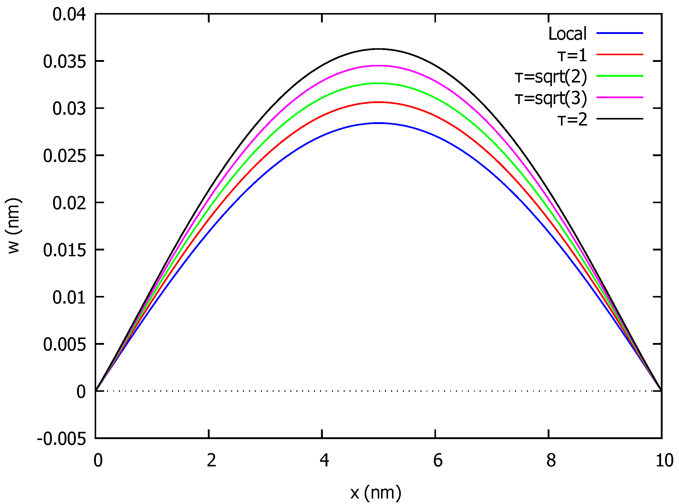
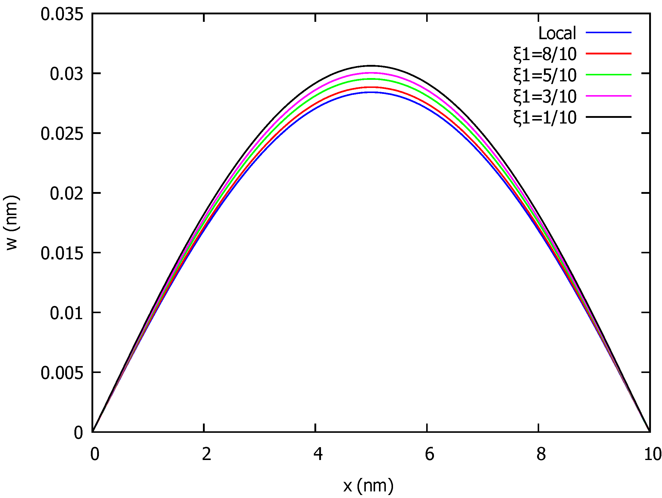
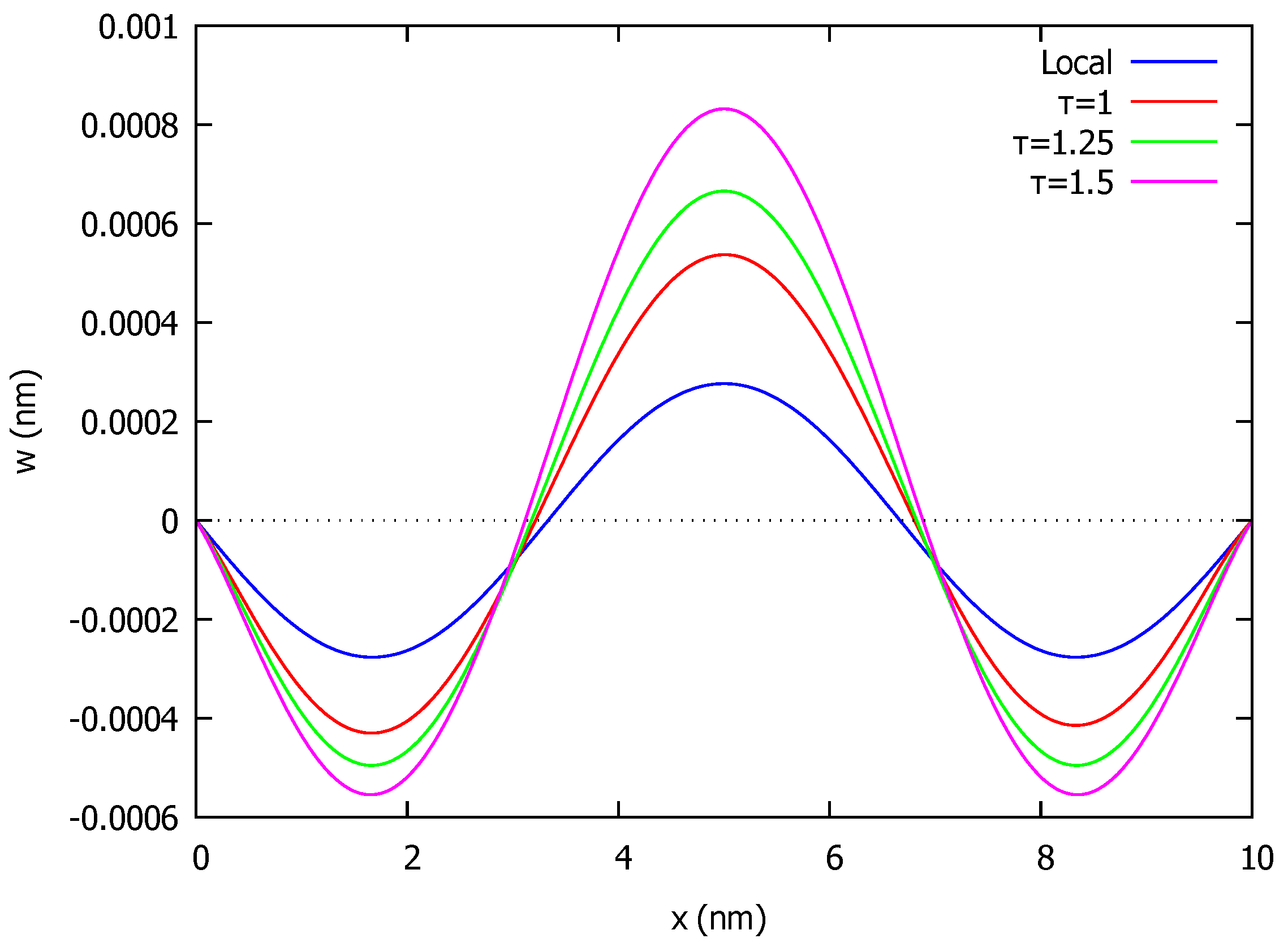
5. Examples and Discussion

Consider a simply supported beam (SS) with length L, height h, width b and Young’s modulus E as given in

Table 1. Geometry, loading and material parameters of the nanobeam.

L (nm)	b (nm)	h (nm)	${\mathit{q}}_0$ (nN/nm)	E (TPa)	$\mathit{\tau }={\mathit{e}}_0\mathit{a}$ (nm)	${\mathit{\xi }}_1$
10	1	1	${10}^{-4}$	5.5	$[1.0,2.0]$	$[0.1,1]$

, see [23]. The value ranges for the nonlocal material constant $\tau$ and the control parameter ${\xi }_1$ (${\xi }_1+{\xi }_2=1$), as well as a load intensity parameter $q_0$ are also displayed in the same table.

It is noted that in [20], it is reported that the nonlocal effect is noticeable when the length of the structure is less than 20 nm and $e_{0}a<2.1$ nm is proposed, while Eringen [12] recommended the value for the parameter $e_0=0.39$.

The bending behavior of the simply supported beam in Eringen’s two phase nonlocal integral model of Euler–Bernoulli elastic beams under a transverse distributed load $q\left(x\right)$ is described by the fourth order Equation (23) with the four boundary conditions (25) where the unknown function is the transverse displacement (deflection) $w\left(x\right)$. In the case of the Helmholtz type kernel (22), the closed form solution of the boundary value problem (23), (25) is delivered by the Algorithm in Algorithm 1. The Algorithm was implemented in the free general purpose sofware Maxima Computer Algebra System.

First, we consider the case of uniformly distributed loading, that is $q\left(x\right)=q_0$. Giving $L,I,E,\tau ,{\xi }_1$ and $q\left(x\right)$ to the Algorithm and after execution we obtain the transverse displacement $w\left(x\right)$ in an exact analytic form.

In Figure 1, we depict the transverse displacement (deflection) of the simply supported beam along its length for both the classical (local) elasticity (${\xi }_1=1$) and the nonlocal elasticity (${\xi }_1=0.1$) for several values of the material parameter $\tau$. As expected, the deformation in the nonlocal theory is greater than in the classical one. In addition, in the nonlocal theory the deformation becomes greater as the material parameter $\tau$ increases, which is also consistent with the softening effect reported in the literature [25,28].

Figure 2 shows the effect of the nonlocal model on the beam deformation, which is controlled by the parameter ${\xi }_2=1-{\xi }_1$, for $\tau =2$. As expected, as ${\xi }_1$ approaches the unit, the solution convergences on the classical (local) solution.

As a second example, we consider the case of a simply supported beam loaded by a variable distributed load given by

$$q\left(x\right)=-q_{0}sin\left(3\pi \frac{x}{L}\right).$$

By entering this load function together with the geometric and material parameters in Table 1 in the Algorithm, we obtain the transverse displacement (deflection) $w\left(x\right)$ in exact explicit form.

Figure 3 shows how the beam is deformed along its entire length in nonlocal theory (${\xi }_1=0.1$) for different values of the nonlocal material parameter $\tau$ and compared to the resulting curve in classical (local) theory (${\xi }_1=1$). Again, the results are as expected and reported in the literature and the softening effect is greater with increasing values of the parameter $\tau$.

6. Conclusions

There is the need for the development of analytical methods for solving integro-differential equations that model numerous situations in science and engineering.

In this paper, a direct operator method for solving in closed form the linear convolution type Volterra–Fredholm integro-differential equations (VFIDE) of the second kind has been presented. The novelty and the main advantages of the proposed method are that it calculates the exact closed form solution of the VFIDE, it is easy to implement to any symbolic algebra system and it is cheap and easy to use. The disadvantages are that it requires the direct and the inverse Laplace transform of the functions and the exact analytic calculation of the integrals involved.

The method has been applied to obtain the exact closed form solution of the fourth order integro-differential equation that models the bending behavior of the beams in the two phase nonlocal integral model of Eringen’s nonlocal elasticity. An algorithm has been developed to construct the solution in the case of a simply supported beam subject to different types of distributed transverse loads.

The work presented will be of interest to scientists and engineers for the symbolic computation of the exact solution of VFIDE and the easy construction of closed form solutions for beam type structures in nonlocal elasticity.

The technique can be extended to solve beam problems with other types of loads and boundary conditions as well as other problems. In preparation of the final version of this paper, a sequel to this work was published by the author, which deals with the closed form solution of three more boundary value problems for the cantilever beam (CF), the clamped pinned beam (CP) and the clamped beam (CC) [47].

References

1. Fleck, N.A.; Muller, G.M.; Ashby, M.F.; Hutchinson, J.W. Strain gradient plasticity: Theory and experiment. Acta Metall. Mater. 1994, 42, 475–487. [Google Scholar] [CrossRef]
2. Lam, D.C.C.; Yang, F.; Chong, A.C.M.; Wang, J.; Tong, P. Experiments and theory in strain gradient elasticity. J. Mech. Phys. Solids 2003, 51, 1477–1508. [Google Scholar] [CrossRef]
3. Cosserat, E. Théorie des Corps Déformables; Librairie Scientifique A. Hermann et Fils: Paris, France, 1909. [Google Scholar]
4. Mindlin, R.D. Influence of couple stresses on stress concentrations. Exp. Mech. 1963, 3, 1–7. [Google Scholar] [CrossRef]
5. Eringen, A.C. Linear theory of micropolar elasticity. J. Math. Mech. 1966, 15, 909–923. [Google Scholar]
6. Mindlin, R.D.; Eshel, N.N. On first strain-gradient theories in linear elasticity. Int. J. Solids Struct. 1968, 4, 109–124. [Google Scholar] [CrossRef]
7. Aifantis, E. Update on a class of gradient theories. Mech. Mater. 2003, 35, 259–280. [Google Scholar] [CrossRef]
8. Providas, E.; Kattis, M.A. Finite element method in plane Cosserat elasticity. Comput. Struct. 2002, 80, 2059–2069. [Google Scholar] [CrossRef]
9. Lee, J.D.; Li, J. Advanced Continuum Theories and Finite Element Analyses; World Scientific: Singapore, 2020; p. 524. [Google Scholar] [CrossRef]
10. Tuna, M.; Leonetti, L.; Trovalusci, P.; Kirca, M. ‘Explicit’ and ‘Implicit’ Non-local Continuum Descriptions: Plate with Circular Hole. In Size-Dependent Continuum Mechanics Approaches; Ghavanloo, E., Fazelzadeh, S.A., Marotti de Sciarra, F., Eds.; Springer: Cham, Switzerland, 2021. [Google Scholar] [CrossRef]
11. Deng, G.; Dargush, G.F. Mixed variational principle and finite element formulation for couple stress elastostatics. Int. J. Mech. Sci. 2021, 202–203, 106497. [Google Scholar] [CrossRef]
12. Eringen, A.C. On differential equations of nonlocal elasticity and solutions of screw dislocation and surface waves. J. Appl. Phys. 1983, 54, 4703. [Google Scholar] [CrossRef]
13. Eringen, A.C. Theory of nonlocal elasticity and some applications. Re. Mech. 1987, 21, 313–342. [Google Scholar]
14. Altan, S.B. Uniqueness of initial-boundary value problems in nonlocal elasticity. Int. J. Solids Struct. 1989, 25, 1271–1278. [Google Scholar] [CrossRef]
15. Polizzotto, C. Nonlocal elasticity and related variational principles. Int. J. Solids Struct. 2001, 38, 7359–7380. [Google Scholar] [CrossRef]
16. Arash, B.; Wang, Q. A review on the application of nonlocal elastic models in modeling of carbon nanotubes and graphenes. Comput. Mater. Sci. 2012, 51, 303–313. [Google Scholar] [CrossRef]
17. Eltaher, M.A.; Khater, M.E.; Emam, S.A. A review on nonlocal elastic models for bending, buckling, vibrations, and wave propagation of nanoscale beams. Appl. Math. Model. 2016, 40, 4109–4128. [Google Scholar] [CrossRef]
18. Eptaimeros, K.G.; Koutsoumaris, C.C.; Tsamasphyros, G.J. Nonlocal integral approach to the dynamical response of nanobeams. Int. J. Mech. Sci. 2016, 115–116, 68–80. [Google Scholar] [CrossRef]
19. Peddieson, J.; Buchanan, G.R.; McNitt, R.P. Application of nonlocal continuum models to nanotechnology. Int. J. Eng. Sci. 2003, 41, 305–312. [Google Scholar] [CrossRef]
20. Wang, Q.; Liew, K.M. Application of nonlocal continuum mechanics to static analysis of micro- and nano-structures. Phys. Lett. A 2007, 363, 236–242. [Google Scholar] [CrossRef]
21. Reddy, J.N. Nonlocal theories for bending, buckling and vibration of beams. Int. J. Eng. Sci. 2007, 45, 288–307. [Google Scholar] [CrossRef]
22. Wang, C.M.; Kitipornchai, S.; Lim, C.W.; Eisenberger, M. Beam bending solutions based on nonlocal Timoshenko beam theory. J. Eng. Mech. 2008, 134, 475–481. [Google Scholar] [CrossRef]
23. Nguyen, N.T.; Kim, N.I.; Lee, J. Mixed finite element analysis of nonlocal Euler-Bernoulli nanobeams. Finite Elem. Anal. Des. 2015, 106, 65–72. [Google Scholar] [CrossRef]
24. Challamel, N.; Wang, C.M. The small length scale effect for a non-local cantilever beam: A paradox solved. Nanotechnology 2008, 19, 345703. [Google Scholar] [CrossRef] [PubMed]
25. Fernández-Sáez, J.; Zaera, R.; Loya, J.A.; Reddy, J.N. Bending of Euler–Bernoulli beams using Eringen’s integral formulation: A paradox resolved. Int. J. Eng. Sci. 2016, 99, 107–116. [Google Scholar] [CrossRef] [Green Version]
26. Polyanin, A.D.; Manzhirov, A.V. Handbook of Integral Equations, 2nd ed.; Chapman and Hall/CRC: New York, NY, USA, 2008. [Google Scholar] [CrossRef]
27. Tuna, M.; Kirca, M. Exact solution of Eringen’s nonlocal integral model for bending of Euler-Bernoulli and Timoshenko beams. Int. J. Eng. Sci. 2016, 105, 80–92. [Google Scholar] [CrossRef]
28. Wang, Y.B.; Zhu, X.W.; Dai, H.H. Exact solutions for the static bending of Euler-Bernoulli beams using Eringen’s two-phase local/nonlocal model. AIP Adv. 2016, 6, 085114. [Google Scholar] [CrossRef] [Green Version]
29. Khodabakhshi, P.; Reddy, J.N. A unified integro-differential nonlocal model. Int. J. Eng. Sci. 2015, 95, 60–75. [Google Scholar] [CrossRef] [Green Version]
30. Adomian, G.; Rach, R. On linear and nonlinear integro-differential equations. J. Math. Anal. Appl. 1986, 113, 199–201. [Google Scholar] [CrossRef] [Green Version]
31. Brunner, H. The numerical treatment of ordinary and partial Volterra integro-differential equations. In Proceedings of the First International Colloquium on Numerical Analysis, Plovdiv, Bulgaria, 13–17 August 1992; De Gruyter: Berlin, Germany, 1993; pp. 13–26. [Google Scholar] [CrossRef]
32. Wazwaz, A.M. A reliable algorithm for solving boundary value problems for higher-order integro-differential equations. Appl. Math. Comput. 2001, 118, 327–342. [Google Scholar] [CrossRef]
33. Bahuguna, D.; Ujlayan, A.; Pandey, D.N. A comparative study of numerical methods for solving an integro-differential equation. Comput. Math. Appl. 2009, 57, 1485–1493. [Google Scholar] [CrossRef] [Green Version]
34. Noeiaghdam, S. Numerical solution of nth-order Fredholm integro-differential equations by integral mean value theorem method. Int. J. Pure Appl. Math. 2015, 99, 277–287. [Google Scholar] [CrossRef] [Green Version]
35. Providas, E. Approximate solution of Fredholm integral and integro-differential equations with non-separable kernels. In Approximation and Computation in Science and Engineering, Springer Optimization and Its Applications 180; Daras, N.J., Rassias, T.M., Eds.; Springer: Cham, Switzerland, 2021; pp. 697–712. [Google Scholar] [CrossRef]
36. Căruntu, B.; Paşca, M.S. Approximate Solutions for a Class of Nonlinear Fredholm and Volterra Integro-Differential Equations Using the Polynomial Least Squares Method. Mathematics 2021, 9, 2692. [Google Scholar] [CrossRef]
37. Wazwaz, A.M. Volterra-Fredholm Integro-Differential Equations. In Linear and Nonlinear Integral Equations; Springer: Berlin/Heidelberg, Germany, 2011; pp. 285–309. [Google Scholar] [CrossRef]
38. Reutskiy, S.Y. The backward substitution method for multipoint problems with linear Volterra–Fredholm integro-differential equations of the neutral type. J. Comput. Appl. Math. 2016, 296, 724–738. [Google Scholar] [CrossRef]
39. Rohaninasab, N.; Maleknejad, K.; Ezzati, R. Numerical solution of high-order Volterra–Fredholm integro-differential equations by using Legendre collocation method. Appl. Math. Comput. 2018, 328, 171–188. [Google Scholar] [CrossRef]
40. Turkyilmazoglu, M. High-order nonlinear Volterra–Fredholm-Hammerstein integro-differential equations and their effective computation. Appl. Math. Comput. 2014, 247, 410–416. [Google Scholar] [CrossRef]
41. Dehestani, H.; Ordokhani, Y.; Razzaghi, M. Combination of Lucas wavelets with Legendre-Gauss quadrature for fractional Fredholm-Volterra integro-differential equations. J. Comput. Appl. Math. 2021, 382, 113070. [Google Scholar] [CrossRef]
42. Berenguer, M.I.; Gámez, D.; López Linares, A.J. Fixed point techniques and Schauder bases to approximate the solution of the first order nonlinear mixed Fredholm-Volterra integro-differential equation. J. Comput. Appl. Math. 2013, 252, 52–61. [Google Scholar] [CrossRef]
43. Parasidis, I.N.; Providas, E. Extension Operator Method for the Exact Solution of Integro-Differential Equations. In Contributions in Mathematics and Engineering: In Honor of Constantin Carathéodory; Pardalos, P.M., Rassias, T.M., Eds.; Springer International Publishing: Cham, Switzerland, 2016; pp. 473–496. [Google Scholar] [CrossRef]
44. Parasidis, I.N.; Providas, E. On the Exact Solution of Nonlinear Integro-Differential Equations. In Applications of Nonlinear Analysis. Springer Optimization and Its Applications; Rassias, T., Ed.; Springer: Cham, Switzerland, 2018; Volume 134, pp. 591–609. [Google Scholar] [CrossRef]
45. Baiburin, M.M.; Providas, E. Exact Solution to Systems of Linear First-Order Integro-Differential Equations with Multipoint and Integral Conditions. In Mathematical Analysis and Applications; Springer Optimization and Its Applications; Rassias, T.M., Pardalos, P.M., Eds.; Springer: Cham, Switzerland, 2019; Volume 154, pp. 1–16. [Google Scholar] [CrossRef]
46. Zwillinger, D. Handbook of Differential Equations, 3rd ed.; Academic Press: San Diego, CA, USA, 1998. [Google Scholar]
47. Providas, E. Closed-Form Solution of the Bending Two-Phase Integral Model of Euler-Bernoulli Nanobeams. Algorithms 2022, 15, 151. [Google Scholar] [CrossRef]
Figure 1. Deflectionof simply supported beam under uniform load and various values of τ .
Appliedmath 02 00017 g001
Figure 2. Deflectionof simply supported beam under uniform load and several values of ξ 1 .
Appliedmath 02 00017 g002
Figure 3. Deflectionof simply supported beam subject to variable load and different values of τ .
Appliedmath 02 00017 g003