One-Dimensional Matter Waves as a Multi-State Bit

Abstract

We design a simple technique to control the position of a localized matter wave. Our system is composed of two counter-phased periodic potentials and a third optical lattice, which can be either periodic or disordered. The only control needed on the system is a three-state switch that allows the sudden selection of the desired potential. The method is proposed as a possible new alternative to achieving the realization of a multi-state bit. We show that this framework is robust, and that the multi-state bit behavior can be observed under weak assumptions. Given the current degree of development of matter wave control in optical lattices, we believe that the proposed device would be easily reproducible in a laboratory, allowing for testing and industrial applications.

1. Introduction

Nowadays, Bose–Einstein condensates (BEC) [1,2,3,4] are routinely used in combination with optical potentials to have direct access to the fundamental quantum behaviors on a macroscopic scale. The state of the art offers a wide range of possibilities in terms of manipulation over these systems [5,6,7,8,9,10,11,12,13,14,15,16,17,18,19,20,21,22,23], and there is a deep knowledge of the expected behaviors from the theoretical side.

The dimensionality of the system can be reduced by flattening the BEC (effective 2D system [14]) or elongating it (effective 1D system [11,12,13]). In the 1D case, interesting boundary conditions can be realized: the elongated BEC can be trapped in a box [15], in a torus [24], or in a harmonic trap [9,10], among other possibilities [7,8].

Many different optical potentials are achievable for this system. Without any presumption of being exhaustive, we recall the possibility of generating both periodic [11,12,13,14] and disordered [16,17,18,19,20,21,22,23,25,26,27] lattices. The latter family of potentials has been employed to observe Anderson localization phenomena [16,17,21,22,27]. One-dimensional speckle potentials, in particular, have been the object of an intensive study in recent years, both from the theoretical and experimental sides. The localization properties of a speckle system have been investigated both in infinitely extended [17,18] and box-bounded systems [26,27], showing that the finite length case can have an even stronger degree of localization compared to the infinite length case, under the proper conditions [27]. In addition to the wide selection of feasible optical potentials, we recall the recent possibility of painting an arbitrary shape time-averaged optical dipole potential [7].

Finally, the Fano–Feshbach resonances [28,29,30] can be employed to lessen or even eliminate the nonlinear effects of the self-interaction, leading to the dynamics of the system being ruled by a linear Schrödinger equation.

This remarkable degree of control over a quantum system allows for the research of technological applications. In particular, investigations into using matter waves as quantum switches or quantum information devices have been made in recent years [31,32,33]. This article proposes a general technique to employ a 1D BEC, either self-interacting or not, as a multi-state bit, by a proper temporal alternation of three optical potentials. This design is entirely new, to the best of our knowledge, and it is the first example of BEC used as a classical multi-state bit. Indeed, unlike the other time-dependent optical potentials proposed to control atoms’ positions, this forces the localized wave function to follow a cyclic sequence of configurations by repeating the same operation on the system, regardless of the initial localization position. The proposed technique is robust and straightforward and can be applied under a broad range of specifications, both in the box and the torus cases. In addition, the number of states is an arbitrary choice.

Considering the complexity of the BEC’s self-interacting dynamics, no closed-form result is proposed. Indeed, the investigation is purely numerical, and the chosen specifications cope with the features of a realistic system, easily reproducible in a laboratory at present.

The paper is organized as follows. Section 2 defines the considered system and outlines its general features. Section 3 discusses how the system can be employed as a multi-state bit, given a simplified set of assumptions. The robustness of the system is investigated in Section 4, where alternative implementations are compared, and an assumption previously considered in Section 3 is weakened to investigate the system’s behavior in a more realistic context. The main results of this work are summarized in Section 5.

2. Model and Methods

Let us consider a non-interacting matter wave in a 1D optical potential. The potential can be selected amongst three possible choices. The system is finite and its length is L. The hamiltonian of the system can be written in a dimensionless form as

$$\widehat{H}=-\frac{d^2}{d{x}^2}+\sum _{k=0}^3{1\mathrm{I}}_{\{k=c\}}{v}_k(x,s_k),$$

(1)

where $c\in \{1,2,3\}$ is a switch that allows the system’s user to select the potential. The three selectable potentials $v_k$ ($k=1\dots 3$) are defined in the remainder of this section. We consider also a zeroth case ($k=0$) which is not selectable during the time evolution of the system, but is needed to set the initial conditions. The Hamiltonian in Equation (1) is dimensionless because it is scaled by a specific energy value $E_{\xi }$, which is related to $v_1(x,s_1)$ and introduced together with it in Section 2.1.

It is reasonably assumed that c can be changed instantaneously, considering that $v_k(x,s_k)$ ($k=0\dots 3$) are optically generated. Numerical results that cope with this assumption are presented in Section 3. When considering the time evolution and the presence of self-interaction, the system is fully described by the Schrödinger equation:

$$i\frac{\partial }{\partial \tau }\psi =\left[\widehat{H}+2\alpha \beta \frac{{\left|\psi \right|}^2}{{\sigma }^2}+\alpha \left({\sigma }^2+{\sigma }^{-2}\right)\right]\psi ,$$

(2)

where $\tau =E_{\xi }t/\hslash$ is a scaled dimensionless time and ${\sigma }^2(x,\tau )=\sqrt{1+{\beta \left|\psi (x,\tau )\right|}^2}$. $\alpha$ and $\beta$ are defined and fully specified in Appendix A. The nonlinear terms describe the self interaction of the Bose–Einstein Condensate (BEC) that can be used in order to realize the system. Equation (2) is an effective 1D model known as non-polynomial Schrödinger equation (NPSE) [34]. This is obtained from the Gross–Pitaevskii 3D equation [35] in order to provide an approximate description for the BEC dynamics under radial confinement. Presently, the self interaction can be chosen to be repulsive ($\beta >0$) [36,37], attractive ($\beta <0$) [28,29] or absent ($\beta =0$) [30], depending on the experimental settings.

The remainder of this section completes the description of the system and is organized as follows. Section 2.1 introduces the features of the optical potentials $v_k,k\in \{0\dots 3\}$ considered in Equations (1) and (2). Section 2.2 compares the instantaneous switch among potentials to other finite-time alternate assumptions, the latter being numerically investigated in Section 4. Section 2.3 introduces the observable quantities needed to assess the system’s state. Finally, Section 2.4 discloses details regarding the numerical methods chosen in simulating the system and its temporal evolution.

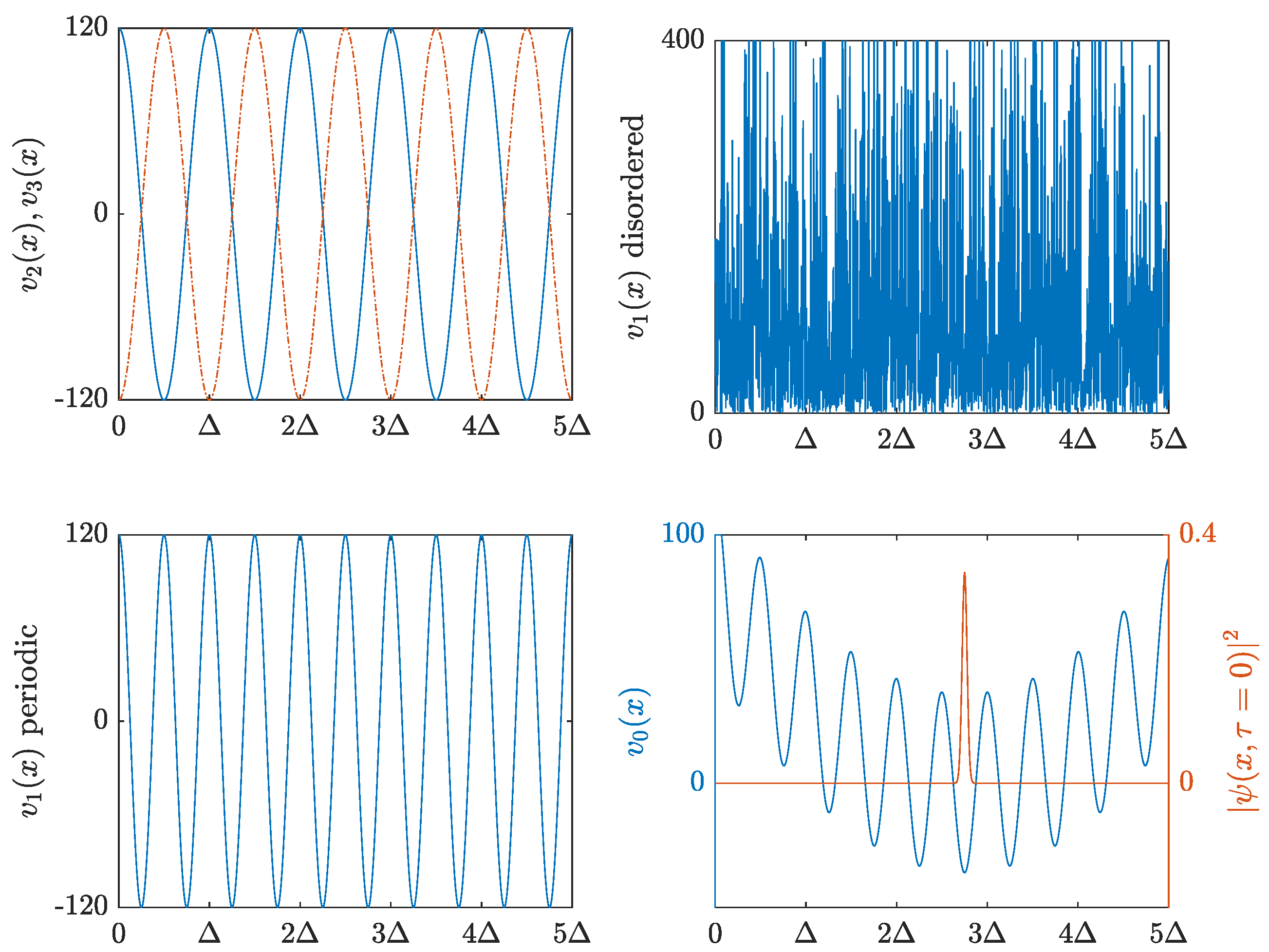
2.1. Optical Potentials

The Hamiltonian $\widehat{H}$ introduced in Equation (1) is specified by considering the potentials described in the following.

$\left(v_1\right)$

The potential $v_1$ is employed in order to keep ${\left|\psi (x,\tau )\right|}^2$ stable over time. To this end, we consider two possibilities: a disodered potential $v_1^d$ and a periodic potential $v_1^p$.

The disordered case. The potential is produced by generating an optical speckle $v_1^d\left(x\right)=V_{0}v(x/\xi )$, with intensity $V_0=〈v_1^d〉$ and autocorrelation length $\xi$[25,38]. The probability distribution of $v\left(x\right)$ is $e^{-v}$. Moreover, it holds that:

$${\langle v\left(y\right)v(y+x)\rangle }_y=1+sin{c}^2\left(\frac{x}{\xi }\right).$$

(3)

An optical speckle is obtained by transmitting a laser beam through a medium with a random phase profile, such as a ground glass plate. The resulting complex electric field is a sum of independent random variables and forms a Gaussian process. Atoms experience a random potential proportional to the intensity of the field. $V_0$ can be either positive or negative, the potential resulting in a series of barriers or wells. However, in both cases, it is possible to observe Anderson localization phenomena [26,27]. The autocorrelation length $\xi$ represents a natural scale for the system and $E_{\xi }:={\hslash }^2/2m{\xi }^2$ is the corresponding energy scale. We define:

$$v_1^d(x,s_1):=s_{1}v\left(x\right),$$

(4)

where $s_1=V_0/E_{\xi }$ is a rescaled dimensionless intensity. The speckle pattern can be generated numerically as discussed in [25] (and references therein).

The ordered case. A smooth, periodic potential $v_1^p(x,s_1)$ can be used as well to maintain ${\left|\psi (x,\tau )\right|}^2$ as stable over time, depending on the considered $\psi (x,\tau )$.

$$v_1^p(x,s_1):=s_{1}f\left(\mathrm{mod}\left(x,\frac{\Delta }{2}\right)\right),$$

(5)

where $\Delta =L/N$ ($N\in \mathbb{N}$), $f(\Delta /2+x)=f(\Delta /2-x)$, and $df\left(x\right)/dx=0\iff$$\mathrm{mod}(x,\Delta /2)=0$. Adopting a common notation, $\mathrm{mod}(a,b)$ stands for the remainder of $a/b$.

In Section 4, we consider $v_1^p(x,s_1)=s_{1}cos\left(\frac{4\pi }{\Delta }x\right)$ as a realistic case.

$\left(v_2\right)$

$v_2$ can be obtained from $v_1^p$ by doubling the period and considering a different amplitude $s_2$, which is a parameter independent from $s_1$.

$$v_2(x,s_2):=s_{2}f\left(\mathrm{mod}(x,\Delta )\right),$$

(6)

where the same requirements described above hold. In Section 4, we consider $v_2(x,s_1)=s_{2}cos(\frac{2\pi }{\Delta }x)$ as a realisitic case.

$\left(v_3\right)$

Additionally, the third potential is smooth and periodic, and in antiphase with $v_2(x,s_2)$:

$$v_3(x,s_3):=s_{3}f\left(\mathrm{mod}(x,\Delta )+\frac{\Delta }{2}\right).$$

(7)

In the following, we will always consider $s_2=s_3$ only.

$\left(v_0\right)$

The initial condition $\psi (x,\tau =0)$ must be localized around $x_0$ such that $\mathrm{mod}(x_0,\Delta )=\Delta /4$. This can be achieved by forcing the BEC to the ground state of a properly chosen optical potential $v_0(x,s_0)$. In Section 3, we consider:

$$v_0(x,s_0):=s_{0}cos\left(\frac{4\pi }{\Delta }x\right)+{\omega }^2{\left(x-\frac{L}{2}-\frac{\Delta }{4}\right)}^2,$$

(8)

where ${\omega }^2$ is a constant, dimensioned as ${\mathrm{length}}^{-2}$, and valued as $|L^{-1}|$.

In Section 3, we show that the system described above acts as a multi-state bit under two alternative boundary conditions: box and torus.

2.2. The Instantaneous Potential Switch and Alternate Assumptions

In Section 3 and Section 4.1, we discuss the multi-state bit behavior under the assumption that the potential can be changed instantaneously. Let us consider a generic $\tau ={\tau }_0$, when the potential is changed from $v_{c_{old}}$ to $v_{c_{new}}$. Hence, we have:

$$\begin{array}{ccc}\hfill \widehat{H}\left(\tau \right)& =& -\frac{d^2}{d{x}^2}+\sum _k{w}_k\left(\tau \right)v_k(x,s_k),\hfill \\ \hfill w_k\left(\tau \right)& =& {1\mathrm{I}}_{\{k=c_{old}\}}\mathsf{\Theta }\left({\tau }_0-\tau \right)+{1\mathrm{I}}_{\{k=c_{new}\}}\mathsf{\Theta }\left(\tau -{\tau }_0\right).\hfill \end{array}$$

(9)

In Section 4.2, we investigate the effect of a non-instantaneous passage from one potential to another, chosen amongst $v_1$, $v_2$, and $v_3$. Given a finite-time switch lasting ${ϵ}^{\prime }$, we represent it as:

$$w_k^{\left(i\right)}\left(\tau \right)={1\mathrm{I}}_{\{k=c_{old}\}}{f}_i\left({\tau }_0-\tau \right)+{1\mathrm{I}}_{\{k=c_{new}\}}{f}_i\left(\tau -{\tau }_0\right)\tau \in \left({\tau }_0-\frac{{ϵ}^{\prime }}{2},{\tau }_0+\frac{{ϵ}^{\prime }}{2}\right).$$

(10)

where $i\in \{1,2,\dots ,6\}$. The considered switches are summarized in

Table 1. The non-instantaneous switches considered in Equation (10) as an alternate assumption to Equation (9). In each transient plot, the red dashed line represents the temporal evolution of the amplitude $f_i\left({\tau }_0-\tau \right)$, associated to the $c_{old}$-th optical potential, as it approaches to zero. Conversely, blue solid lines represent the amplitude temporal profile $f_i\left(\tau -{\tau }_0\right)$ of the $c_{new}$-th potential that is being activated in ${\tau }_0$.

i	${\mathit{f}}_{\mathit{i}}\left(\mathit{\tau }\right)$	Transient
1	$\frac{\tau +{ϵ}^{\prime }/2}{{ϵ}^{\prime }}$
2	$\frac{\tau }{{ϵ}^{\prime }/2}\mathsf{\Theta }\left(\tau \right)$
3	$\frac{e^{\tau +{ϵ}^{\prime }/2}-1}{e^{{ϵ}^{\prime }}-1}$
4	$\frac{e^{\tau }-1}{e^{{ϵ}^{\prime }/2}-1}\mathsf{\Theta }\left(\tau \right)$
5	$\frac{1+\tanh \left(\frac{2\tau }{{ϵ}^{\prime }}\right)}{2}$
6	$\frac{1+\tanh \left(\frac{4\tau }{{ϵ}^{\prime }}\right)}{2}\mathsf{\Theta }\left(\tau \right)$

. This generalization of $w_k\left(\tau \right)$ improves the realism of our framework and allows us to test the ability of the system to preserve the density profile of the wave function that is localized in $\tau =0$.

The actual transient’s profile and duration would depend on the chosen hardware specifications in a real experiment.

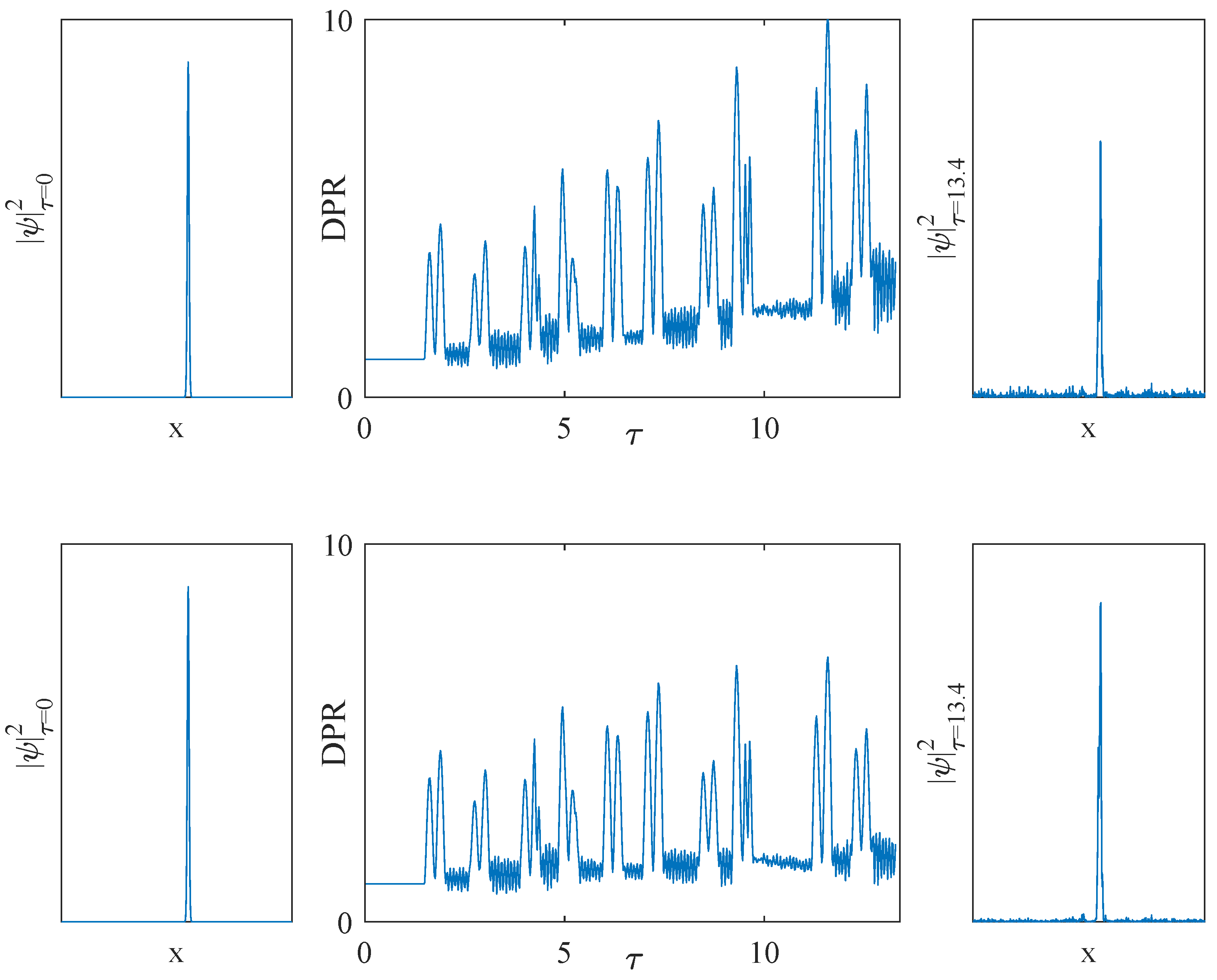
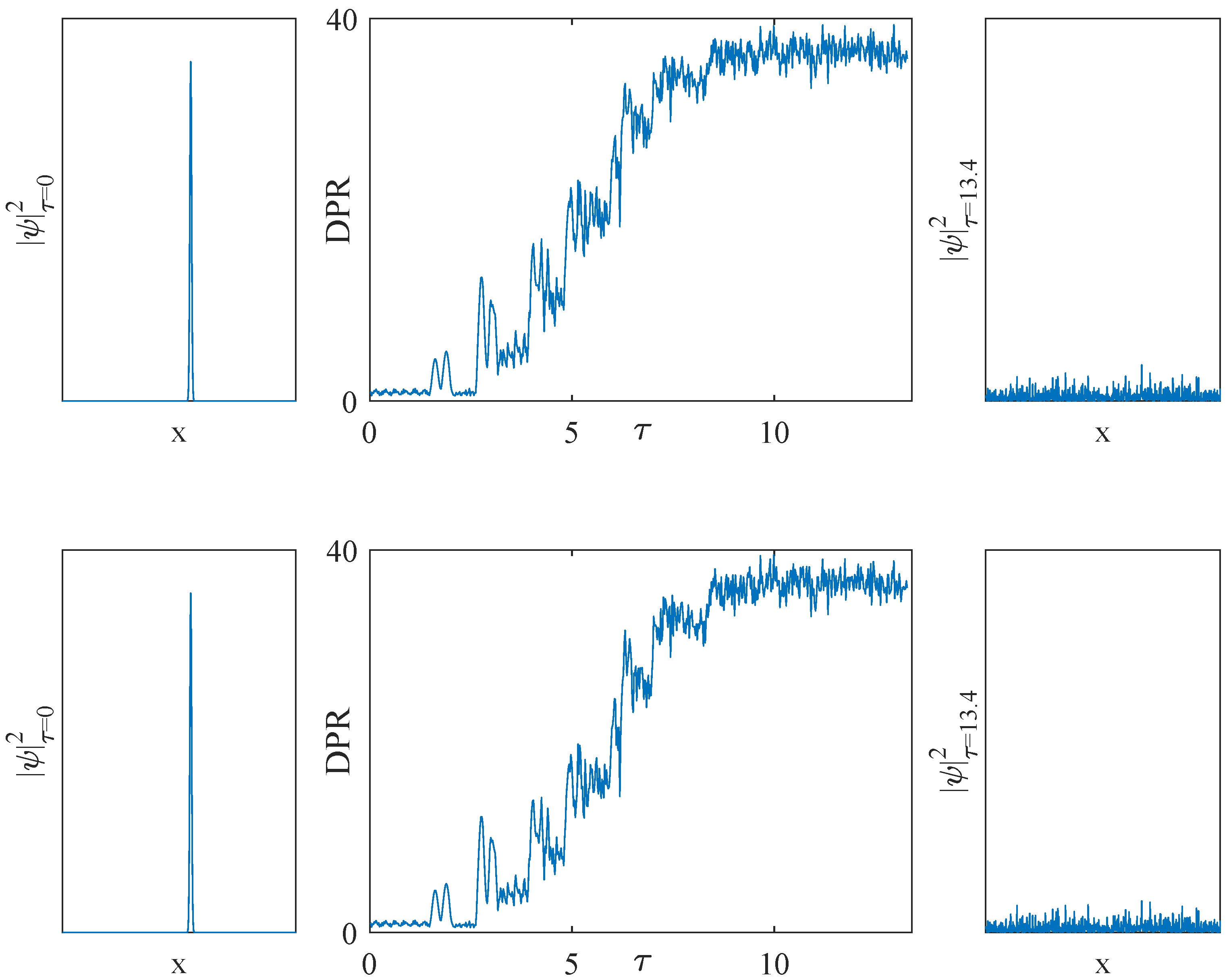
2.3. Measure of System’s State and Stability

As anticipated in Section 2.1, the system is designed to handle the position of a localized matter wave $\psi (x,\tau )$. In this context, the position $x_{loc}$ is defined as the mode of the density profile:

$$x_{loc}\left(\tau \right):=\underset{x\in [0,L]}{\mathrm{argmax}}{\left|\psi (x,\tau )\right|}^2.$$

(11)

In Section 3, we describe a method to control the localization position $x_{loc}$ of the matter wave $\psi$ by changing the c value with proper timing. Hence, we are interested in preventing the spatial expansion of $\psi$, in order to be able to measure $x_{loc}\left(\tau \right)$ even for $\tau \gg 0$. The participation ratio (PR) is commonly used in the literature as a measure of the localization degree [27,39]:

$$\mathrm{P}\mathrm{R}\left[\psi \right]=\frac{1}{L{\int }_{L}dx{\left|\psi \left(x\right)\right|}^4}.$$

(12)

We introduce the following quantity DPR to compare the PR value measured during the system’s evolution against the initial one:

$$\mathrm{DPR}\left(\tau \right)=\frac{\mathrm{P}\mathrm{R}\left[\psi (x,\tau )\right]}{\mathrm{P}\mathrm{R}\left[\psi (x,0)\right]}.$$

(13)

The measure of $x_{loc}\left(\tau \right)$ becomes more difficult and less precise at increasing DPR $\left(\tau \right)$ values. In our system, $x_{loc}$ is clearly measurable when $\mathrm{DPR}\lesssim 10$, while it cannot be defined nor observed anymore when $\mathrm{DPR}\gtrsim 20$.

2.4. Numerical Methods

In the following, some technical details are disclosed regarding the numerical simulations presented in this paper to ease their replicability.

The system is investigated through the numerical integration of Equation (2), given the Hamiltonian specified by Equations (9) and (10), where the considered potentials are described in Section 2.1 and the temporal profiles of a non-instantaneous transient between two subsequent potentials are displayed in Table 1.

The temporal evolution of the potential is chosen by the user, who is able to select $c_{\tau }$ at each instant $\tau$ (finite-time transients discussed in Section 2.2 aside). Thus, a matrix $v(x,\tau )$ is prepared before starting the numerical integration to simulate the external inputs that the matter wave receives by time.

The initial condition $\psi (x,{\tau }_0)$ is chosen as the ground state of the potential $v_0\left(x\right)$, which is obtained by the quantum imaginary time evolution technique (see, e.g., [40] and references therein), as the Hamiltonian is interacting.

Given the deterministic potential evolution $v(x,\tau )$ and the initial condition $\psi (x,{\tau }_0)$, Equation (2) is integrated by applying one among three possible methods:

• in case the system is approximately non-interacting, the Crank–Nicolson [41] or the midpoint [42] integration schemes are considered;
• in case the system is strongly self-interacting, the midpoint integration scheme is still applicable, while the standard Crank–Nicolson scheme is replaced by a modified version that is well defined also in the nonlinear case [43].

By comparing the results obtained from two alternative methods, both in the linear and the nonlinear cases, we implicitly verify the absence of implementation errors that could affect the simulations.

3. How to Use the System as a Multi-State Bit

A multi-state bit can assume a state chosen from a discrete and finite set. We can conventionally define this set of states by partitioning the system into $2N=2L/\Delta$ intervals and labeling each interval with a number $n\in \{1,\dots ,2N\}$. An example of the optical potentials set $\left\{v_k\right\}$ ($k=0\dots 3$), needed to achieve the system in the case $N=5$, is shown in Figure 1. The potentials are applied according to the schema represented in Figure 2.

We need to perform three basic operations on our system in order to consider it a true multi-state bit: writing information, keeping memory of it over an arbitrary time lapse, and reading it again. The latter is introduced in Section 3.1, while the implementation of the writing and storing operations is described in Section 3.2.

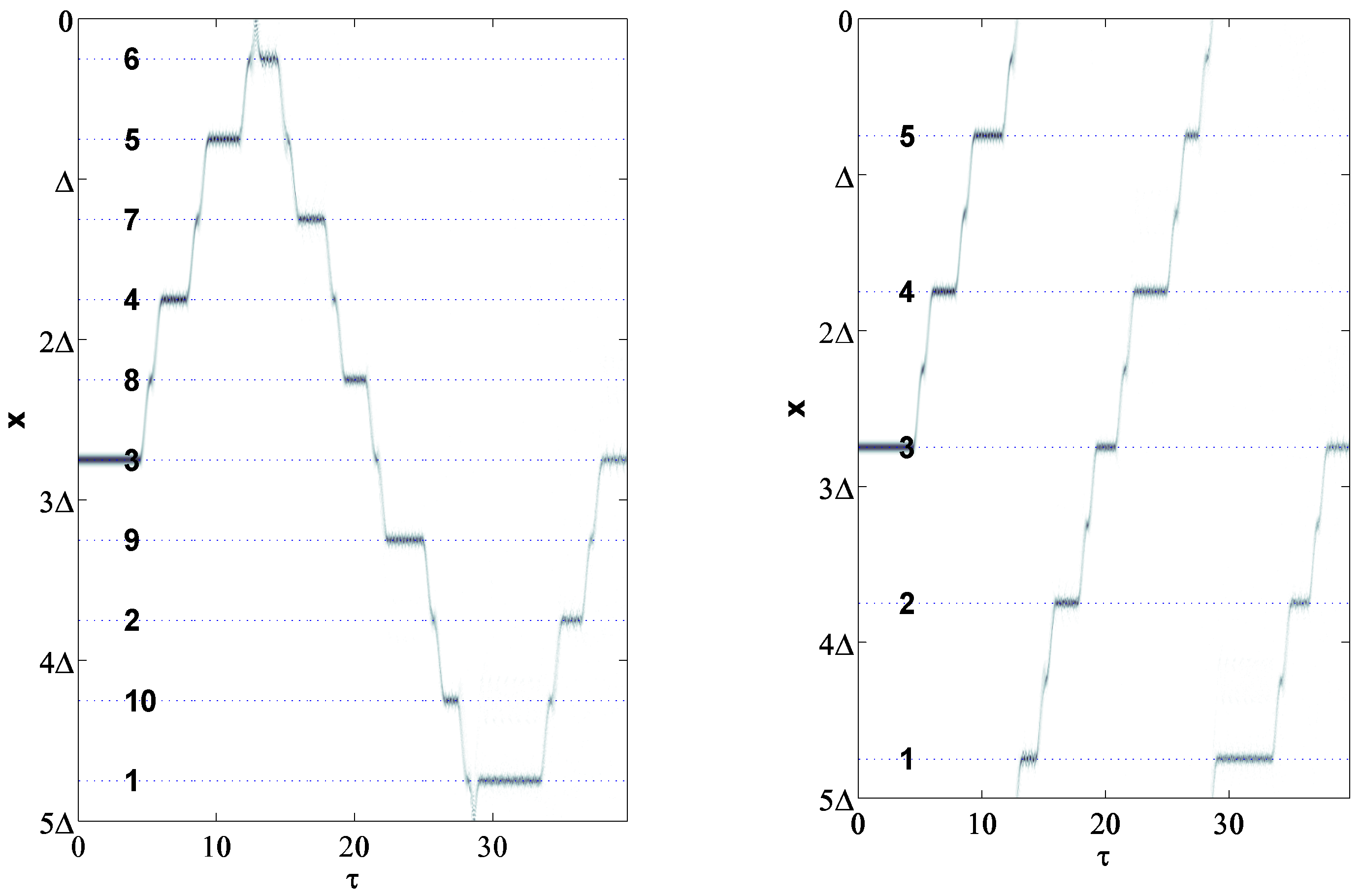
3.1. Reading Information from the Position of a Localized Matter Wave

Using a matter wave allows us to measure the density profile directly. Since the chosen initial condition of the system is a localized state $\psi (x,{\tau }_0)$, most of the density is concentrated in a small region. If $\mathrm{DPR}\left(\tau \right)\lesssim 10$ while the system evolves, we can associate a number $n_j$ to every instant $\tau$ by measuring the density profile, with special reference to the position $x_{loc}$ defined in Equation (11):

$${\phi }_R\left(\psi |\tau \right):=\sum _{j=1}^{2N}{n}_j{1\mathrm{I}}_{\left\{j-1\le \frac{2x_{loc}\left(\tau \right)}{\Delta }<j\right\}}.$$

(14)

The definition reported above allows us to read the information stored in our system. The underlying idea is simple. Indeed, the system’s domain $(0,L)$ must be partitioned in $2N$ intervals, each of them being labeled with a natural number n. If $x_{loc}\left(\tau \right)$ is included in the j-th interval and the operator ${\phi }_R\left(·|\tau \right)$ is applied, the system returns the value $n_j$.

The convenient choice of $n_j$ depends on the boundary conditions. In case of box boundary conditions, we choose:

$$n_j=\frac{j+1}{2}{1\mathrm{I}}_{\left\{\mathrm{mod}\right(j,2)=1\}}+\left(2N-\frac{j}{2}+1\right){1\mathrm{I}}_{\left\{\mathrm{mod}\right(j,2)=0\}}.$$

(15)

In case of toroidal boundary conditions, we choose:

$$n_j=\frac{j+\mathrm{mod}(j,2)}{2}.$$

(16)

The reason for these choices is explained in Section 3.2.3. In our example ($N=5$), Equation (15) leads to:

$$\underline{n}=(1,10,2,9,3,8,4,7,5,6),$$

and Equation (16) leads to:

$$\underline{n}=(1,1,2,2,3,3,4,4,5,5),$$

as shown in Figure 3.

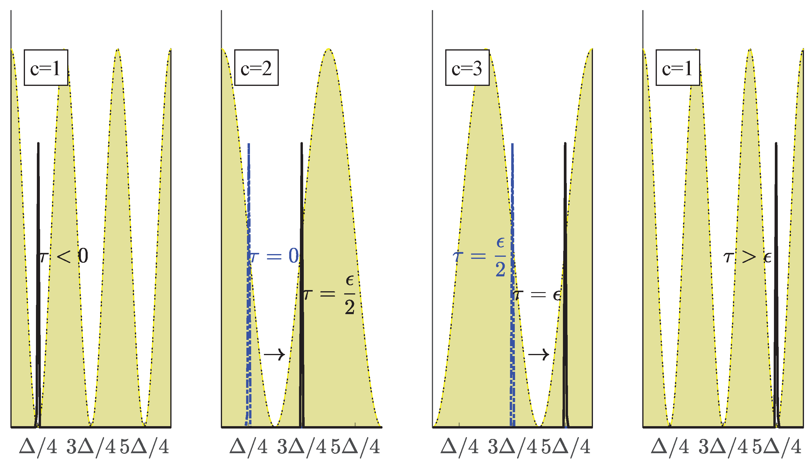
3.2. Writing and Maintaining Information in the System

This section explains how to write information in the system (using operators ${\phi }_{+}$ and ${\phi }_{-}$) and how to store the information over a time lapse $\delta$, keeping $n_{\tau }$ constant (using operator ${\phi }_{\delta }$).

As discussed in Section 2, the only way that we have to influence the system is switching $c_{\tau }$ from one value to another. We aim to use this possibility to define three actions which affect the system as follows:

$$\begin{array}{ccc}\hfill {\phi }_R\left[{\phi }_{+}\left(\psi \right|\tau )|\tau +ϵ\right]& =& {\phi }_R\left(\psi |\tau \right)+1,\hfill \end{array}$$

(17)

$$\begin{array}{ccc}\hfill {\phi }_R\left[{\phi }_{-}\left(\psi \right|\tau )|\tau +ϵ\right]& =& {\phi }_R\left(\psi |\tau \right)-1,\hfill \end{array}$$

(18)

$$\begin{array}{ccc}\hfill {\phi }_R\left[{\phi }_{\delta }\left(\psi \right|\tau )|\tau +\delta \right]& =& {\phi }_R\left(\psi |\tau \right),\hfill \end{array}$$

(19)

where $ϵ$ is the time interval necessary to apply the operators ${\phi }_{\pm }$, and $\delta$ is a time interval over which the information has to be stored in the system. As explained in Section 3.2.3, the boundary conditions affect the definition of the ${\phi }_{+}$ and ${\phi }_{-}$ operators. In case of box conditions, we have:

$${\phi }_R\left[{\phi }_{\pm }\left(\psi \right|\tau )|\tau +ϵ\right]=\mathrm{mod}[{\phi }_R\left(\psi |\tau \right)-1\pm 1,2N]+1.$$

(20)

In case of toroidal conditions, we have:

$${\phi }_R\left[{\phi }_{\pm }\left(\psi \right|\tau )|\tau +ϵ\right]=\mathrm{mod}[{\phi }_R\left(\psi |\tau \right)-1\pm 1,N]+1.$$

(21)

The remainder of Section 3.2 is organized as follows. Section 3.2.1 defines the ${\phi }_{\delta }$ operator, and Section 3.2.2 introduces the ${\phi }_{+}$ and ${\phi }_{-}$ operators. The ${\phi }_{\pm }$ properties are further investigated in Section 3.2.3 and Section 3.2.4. The first highlights the different implications from the two boundary conditions considered (i.e., box and torus), while the latter provides an estimation of the time required to write information on the proposed device, depending on the system’s specifications.

3.2.1. Definition of ${\phi }_{\delta }$

The definition of ${\phi }_{\delta }(·|\tau )$ is based on different principles in case we use $v_1^d$ or $v_1^p$.

In case we use a disordered potential $v_1^d$, it can cause the Anderson localization of the system and it inhibits any transport phenomena. Hence, provided that the disordered potential amplitude is big enough, any localized matter wave $\psi (x,{\tau }_0)$ should remain localized at the same position when observed in ${\tau }_0+\delta$.

In case we use a periodic potential $v_1^p$, it can inhibit any transport phenomena too, provided that the localization point is exactly coincident with a local minimum of the potential and the amplitude is big enough.

In both cases, we can define ${\phi }_{\delta }$ as:

$${\phi }_{\delta }\left(\psi \right|{\tau }_0)={\int }_0^L{\psi }_{y,{\tau }_0}K\left(y,x,{\tau }_0,{\tau }_0+\delta |c_{\tau }=1\right)dy,$$

(22)

where $K(y,x,{\tau }_0,{\tau }_0+\delta )$ is the propagator associated with Equation (2). Figure 2 (first and fourth panels) provides a graphical explanation of ${\varphi }_{\delta }$ when using $v_1^p$.

3.2.2. Definition of ${\phi }_{\pm }$

The definition of ${\phi }_{\pm }(·|\tau )$ is based on the fact that a localized matter wave can experience a periodic potential as the single well where the mass is concentrated, provided that the potential amplitude is big enough and that $x_{loc}$ is near enough to the local minimum $x_{min}$ of the potential. In case of a symmetric well, the symmetry of the eigenstates is well defined and there is a time interval $ϵ/2$, after which it holds that:

$$\psi \left(x,\tau +\frac{ϵ}{2}\right)\simeq \psi \left(x+2(x_{min}-x_{loc}),\tau \right).$$

(23)

Let us suppose that:

$$x_{loc}\left(\tau \right)=x_{min}-\frac{\Delta }{4}-{\delta }_x\mathrm{with}{\delta }_x\ll \Delta .$$

(24)

From Equation (23), we have:

$$x_{loc}\left(\tau +\frac{ϵ}{2}\right)=2x_{min}-x_{loc}\left(\tau \right)=x_{min}+\frac{\Delta }{4}+{\delta }_x.$$

(25)

Applying an instantaneous $\pi$ phase shift to the periodic potential leads to a displacement of the local minimum $x_{min}\to x_{min}^{\prime }=x_{min}+\Delta /2$. Now, we have:

$$x_{loc}\left(\tau +\frac{ϵ}{2}\right)=x_{min}^{\prime }-\frac{\Delta }{4}+{\delta }_x,$$

(26)

and after one more $ϵ/2$ time lapse, we obtain:

$$x_{loc}(\tau +ϵ)=2x_{min}^{\prime }-x_{loc}\left(\tau +\frac{ϵ}{2}\right)=x_{loc}\left(\tau \right)+\Delta .$$

(27)

So, we make the localized matter wave travel a distance $\Delta$ by applying two periodic potentials in anti-phase and with big amplitude. In Section 4, we investigate the conditions under which this displacement can be iterated, preventing $\mathrm{DPR}\left(\tau \right)$ from rising beyond an acceptable level. The discussion above leads to a definition of ${\phi }_{\pm }$:

$$\begin{array}{ccc}\hfill {\phi }_{\pm }\left(\psi \right|{\tau }_0)& :=& {\int }_0^L{\psi }_{y,{\tau }_0}K\left(y,x,{\tau }_0,{\tau }_0+\delta |c_{\tau }=c_{\tau }^{\pm }\right)dy,\hfill \\ \hfill c_{\tau }^{+}& =& 2·{1\mathrm{I}}_{\{\tau \in [{\tau }_0,{\tau }_0+\frac{ϵ}{2}]\}}+3·{1\mathrm{I}}_{\{\tau \in [{\tau }_0+\frac{ϵ}{2},{\tau }_0+ϵ]\}},\hfill \\ \hfill c_{\tau }^{-}& =& 3·{1\mathrm{I}}_{\{\tau \in [{\tau }_0,{\tau }_0+\frac{ϵ}{2}]\}}+2·{1\mathrm{I}}_{\{\tau \in [{\tau }_0+\frac{ϵ}{2},{\tau }_0+ϵ]\}}.\hfill \end{array}$$

(28)

Figure 2 (central panels) gives a graphical explanation of ${\varphi }_{+}$.

3.2.3. ${\phi }_{\pm }$ Near to the Boundaries

The periodic potential in the torus is translation invariant with respect to the transformation $x\mapsto x\pm \Delta$. This implies that the mechanism described in Section 3.2.2 holds in any portion of the system in the same way. This leads to Equation (21). Equation (16) originates from the fact that $x_{loc}$ can be moved only by $\Delta$ long steps, and so there are only N allowed positions where $x_{loc}$ can be found, as shown in Figure 3 (right panel).

On the other hand, the box boundary condition has no translation invariance and the localized matter wave is reflected by the infinite potential walls. As shown in Figure 3, $x_{loc}$ is shifted by $\Delta /2$ near to the boundaries, because $x_{loc}(\tau /2)=x_{loc}\left(\tau \right)$. This fact implies that there are $2N$ allowed positions where $x_{loc}$ can be found. We can enumerate these positions in the order that we obtain them by an iterative application of the ${\varphi }_{+}(·|\tau )$ operator to ${\psi }_{x,{\tau }_0}$. The resulting order is described by Equation (15). An example is shown in Figure 3 (left panel).

Figure 2. Graphical explanation of the effects described in Section 3.2.1 and Section 3.2.2. The proper timing for alternating the three selectable potentials causes the localized matter wave to move and then maintain the new $x_{loc}$.

Figure 2. Graphical explanation of the effects described in Section 3.2.1 and Section 3.2.2. The proper timing for alternating the three selectable potentials causes the localized matter wave to move and then maintain the new $x_{loc}$.

Figure 3. Density plot of ${\left|\psi (x,\tau )\right|}^2$, using the specifications shown in Figure 1 (periodic case $v_1^p$). We applied ${\phi }_{\delta }\circ {\phi }_{+}$ ten times, considering a different random $\delta$ value per application. The same pattern is simulated considering both box (left panel) and boundary (right panel) conditions.

Figure 3. Density plot of ${\left|\psi (x,\tau )\right|}^2$, using the specifications shown in Figure 1 (periodic case $v_1^p$). We applied ${\phi }_{\delta }\circ {\phi }_{+}$ ten times, considering a different random $\delta$ value per application. The same pattern is simulated considering both box (left panel) and boundary (right panel) conditions.

3.2.4. Time Scale of Writing Operations

As the presented system is proposed for practical purposes, it is relevant to investigate the time scale $ϵ$ required for performing each ${\phi }_{\pm }$ operation. To estimate the analytical dependency of $ϵ$ in (28) from the other variables that describe the system, two approximations are required. First, we have to neglect the non-linear contribution of the matter wave’s self-interaction. This is reasonable, as it mainly affects the degree of localization that the matter wave experiences during its motion, while we are interested in estimating the oscillation period of ${\psi }_{x,\tau }$ given the presence of the optical potential $v_2\left(x\right)$ or $v_3\left(x\right)$. Further, while applying ${\phi }_{\pm }$, the matter wave’s center of mass oscillates about a local minimum $x^{\prime }$ of the active potential $v_c\left(x\right)$ ($c=2,3$) during a time interval lasting $ϵ/2$—that is, a half-oscillation period. If we apply a 2nd-order approximation to $v_c(x-x^{\prime })$ ($c=2,3$), each half-oscillation can be regarded as part of a simple harmonic motion. Namely, restoring the S.I. units’ representation by multiplying back the dimensionless potential by the energy scale $E_{\xi }$, we have:

$$\begin{array}{ccc}\hfill v_c(x-x^{\prime })& =& E_{\xi }{s}_{c}cos\left(\frac{4\pi }{\Delta }(x-x^{\prime })\right)\hfill \\ & \approx & 8E_{\xi }{s}_c\frac{{\pi }^2{(x-x^{\prime })}^2}{{\Delta }^2}\hfill \\ & \equiv & \frac{1}{2}m{\omega }^2{(x-x^{\prime })}^2,\hfill \end{array}$$

where $c=2,3$ and the constant terms are omitted, as they are not relevant to the considered problem.

Since a coherent state (such as a non-interacting matter wave) in a harmonic potential behaves as a classical particle with a good degree of approximation, the oscillation period can be estimated as:

$$ϵ\approx \frac{2\pi }{\omega }=\frac{m\Delta \xi }{\hslash \sqrt{2s_c}}.$$

(29)

Equation (29) shows how the operating time scale $ϵ$ can be easily controlled by tuning the parameters $N_a$, $s_c$, and $\Delta$, such that the system’s user is able to decide when constructing the experimental setup. Namely, a lesser mass m of the Bose–Einstein condensate, or a greater amplitude $s_c$ or a smaller spatial period $\Delta$ of the optical potential, implies a smaller $ϵ$, that is, faster writing operations.

Table 2. Examples of time scale $ϵ$ evaluated through approximation (29) under different experimental settings.

${\mathit{N}}_{\mathit{a}}$ (${}^{39}$K Atoms)	$\mathsf{\Delta }$ [$\mathsf{\mu }$m]	${\mathit{s}}_{\mathit{c}}$$\left(1\right)$	$\mathit{ϵ}$ (s)
${10}^4$	30	90	∼$1.2\times {10}^1$
${10}^2$	6	200	∼$1.8\times {10}^{-2}$
${10}^1$	3	400	∼$3.3\times {10}^{-4}$

reports the estimated time scale $ϵ$ given three feasible experimental specifications. Our numerical simulations are in good agreement with the approximated results displayed in the table. It is worth noticing that $ϵ$ is not directly comparable with the corresponding time required to update a ferromagnetic bit, as an arbitrary number of bits must be accessed to increment a generic natural number, depending on its value. On the other hand, a multi-state bit enables representations that are different from the base-2 numeral system.

4. Stability and Robustness of the Multi-State Bit

In this section, we verify the possibility of the system to be used as a multi-state bit under different parameter choices. We compare the results using DPR, defined in Section 2.3. The section aims to identify a stable multi-bit example that can also be feasible in the laboratory.

4.1. Multi-State Bit under Various Settings

We have compared the two considered potential choices $v_1^d$ and $v_1^p$, using them to store information in the system. In case we choose to maintain $c_{\tau }=1$ constant, both of them are equally good at keeping the matter wave localized over time. $v_1^p$ turns out to be better than $v_1^d$ when ${\varphi }_{\pm }$ is applied repeatedly to the system. This is the case when we want to write information to be stored in the system. A numerical example is reported in Figure 4.

When using $v_1^d$, $|s_1|$ must be big enough to keep $\psi (x,\tau )$ localized over time, but not big enough to cause fragmentation phenomena. If the matter wave is fragmented, $\mathrm{DPR}$ increases when $\psi (x,\tau )$ is forced to oscillate ($c_t>1$). Figure 5 (left panel) shows an example of an optimal level of $|s_1|$ when using $v_1^d$. On the other hand, when using $v_1^p$, $s_1$ can be chosen arbitrarily high without fragmenting the matter wave. This is the reason why $v_1^p$ leads to a more stable multi-bit behavior than $v_1^d$.

When considering self-interaction, we observed an increased stability (lower DPR over time) when choosing $\beta <0$, especially if using $v_1^p$ (see Figure 4). Intuitively, $\beta >0$ decreases the stability of the system.

Moreover, all the potential amplitudes must be higher at increasing N values in order to keep $\psi (x,\tau )$ confined in a local fluctuation of the potential when the total number of fluctuations N is bigger. An example of this fact is shown in Figure 5 (right panel). Considering these results, a feasible experimental setting that allows observing a stable ten-states multi-bit could be the following: ${}^{39}$K elongated BEC (${10}^4$ atoms) under box boundary conditions; system dimensions 300 $\mathsf{\mu }$m × 30 $\mathsf{\mu }$m; periodic $v_1^p$ potential; $s_1=s_2=s_3\ge 90$; $N=5$. Please see Appendix A (and references therein) for further details.

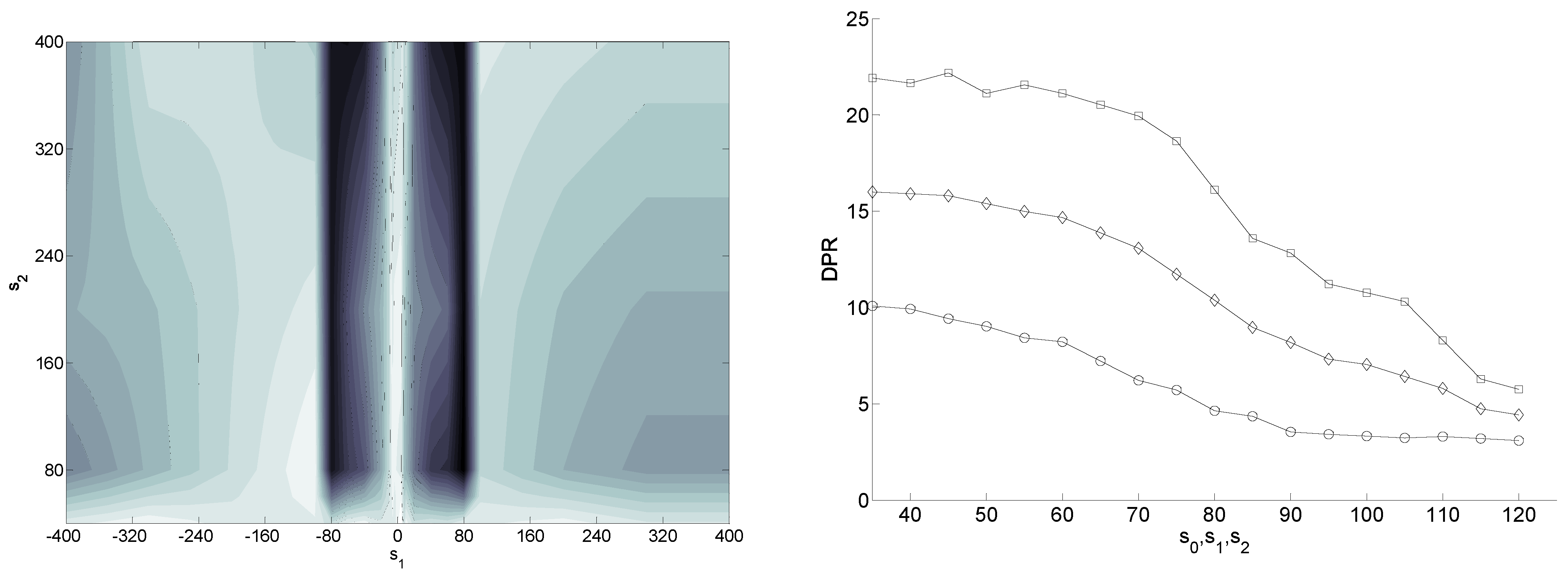
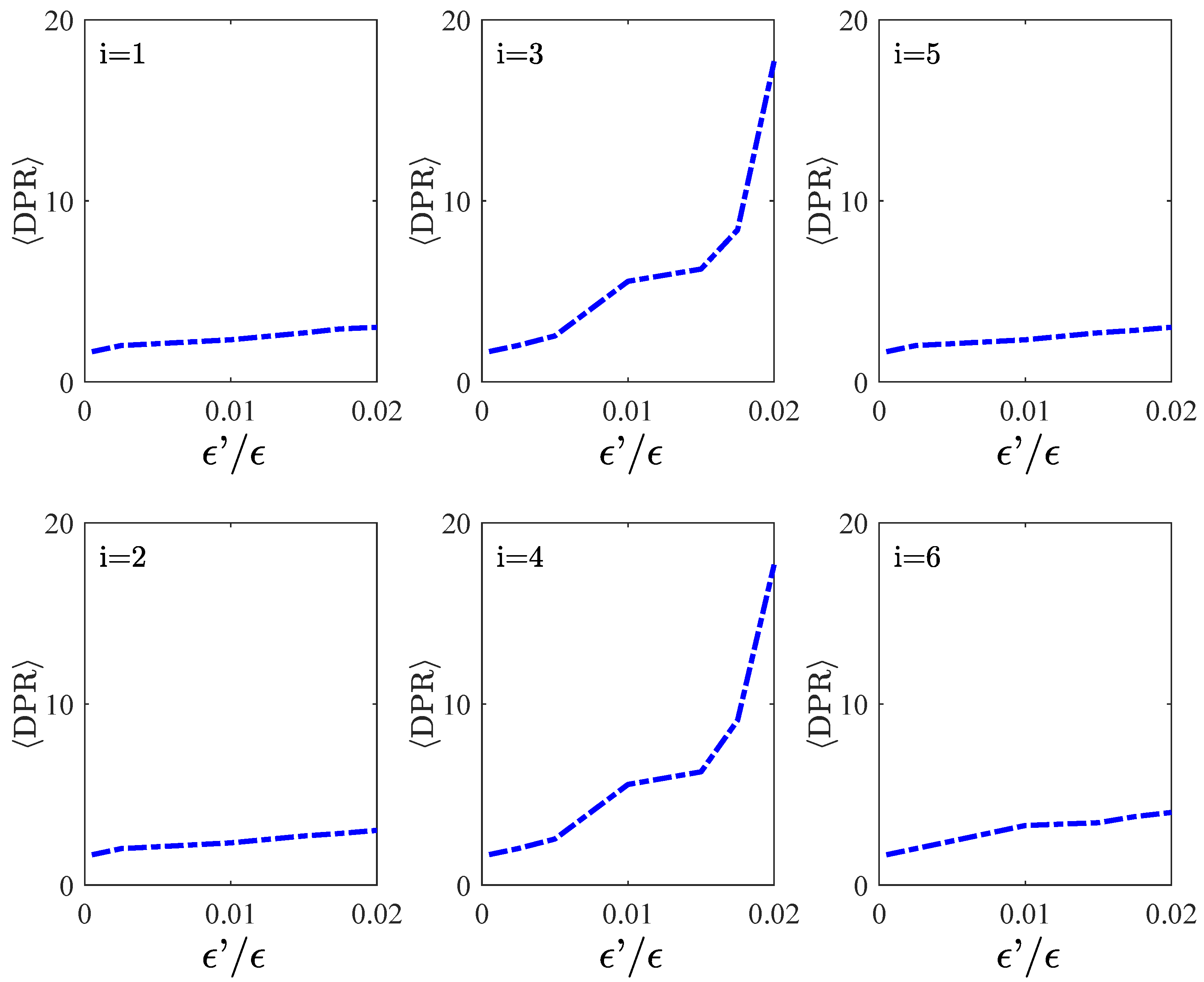
4.2. Multi-State Bit Stability against Potential Imperfections

In Section 4.1, we have found that experimentally feasible multi-state bits are possible under the assumption of instantaneous potential switching. In this section, we discuss how a finite time switch can affect the stability of the system, depending on its duration ${ϵ}^{\prime }$. We restrict ourselves to considering a specific parameter setting which is stable in case ${ϵ}^{\prime }=0$: $\alpha =0.01$; $\beta =-15$; $N=5$; $s_1=s_2=s_3=120$. The time evolution of this system was simulated together with each of the switch shapes defined in Section 2.2, in order to find out to what extent the system remains stable at increasing $\frac{{\epsilon }^{\prime }}{\epsilon }$ values. The considered evolution path is:

$$\psi \left(x,T\right)={◯}_{k=1}^{10}{\phi }_{{\delta }_k}\circ {\phi }_{+}\left[\psi \left(x,0\right)\right],$$

(30)

where the evolution time is $T={\sum }_k{\delta }_k+10ϵ+30{ϵ}^{\prime }$. The first term ${\sum }_k{\delta }_k$ measures the total amount of time throughout which information is stored in the system. The intervals ${\delta }_k$ between the next two writing operations ${\phi }_{+}$ have a random duration, under the boundary ${\sum }_k{\delta }_k=50ϵ$. The second term $10ϵ$ is the total duration of the ten writing operations, except for the finite time switches contribution, which is considered in the third term $30{ϵ}^{\prime }$. We measure $〈\mathrm{DPR}\left[\psi \left(x,T\right)|w^{\left(i\right)},{ϵ}^{\prime }\right]〉$ for all the considered switch shapes ($i=1\dots 6$) and with different switch durations ($\frac{{ϵ}^{\prime }}{ϵ}\in [{10}^{-3},2\times {10}^{-2}]$). $\langle ·\rangle$ is the average over the random paths $\{{\delta }_1,\dots ,{\delta }_{10}\}$. The resulting $〈\mathrm{DPR}\left(w^{\left(i\right)},\frac{{ϵ}^{\prime }}{ϵ}\right)〉$ are shown in Figure 6. If $\frac{{ϵ}^{\prime }}{ϵ}\lesssim {10}^{-2}$, the system remains stable regardless of the chosen switch shape. Otherwise, the system stability depends on the switch shape.

5. Summary

We have developed a technique to change and preserve the position of a localized matter wave. This behavior is directly applicable to obtaining a multi-state memory device. This system can be built using optical potentials already available in the laboratory. The multi-bit behavior can be observed under multiple parameter choices, and we have suggested a fully specified multi-bit that could be realized at present. Given that BECs and optical potentials are currently investigated from a quantum information perspective, this work opens the possibility of turning the same BEC from a q-bit into a classical multi-state bit, and vice versa, in the future.

References

1. Anderson, M.H.; Ensher, J.R.; Matthews, M.R.; Weiman, C.E.; Cornell, E.A. Observation of Bose-Einstein condensation in a dilute atomic vapor. Science 1995, 269, 198. [Google Scholar] [CrossRef] [PubMed] [Green Version]
2. Davis, K.B.; Mewes, M.O.; Andrews, M.R.; van Druten, N.J.; Durfee, D.S.; Kurn, D.M.; Ketterle, W. Bose-Einstein Condensation in a Gas of Sodium Atoms. Phys. Rev. Lett. 1995, 75, 3969. [Google Scholar] [CrossRef] [PubMed] [Green Version]
3. Jin, D.S.; Ensher, J.R.; Matthews, M.R.; Wieman, C.E.; Cornell, E.A. Collective Excitations of a Bose-Einstein Condensate in a Dilute Gas. Phys. Rev. Lett. 1996, 77, 420. [Google Scholar] [CrossRef] [PubMed]
4. Inguscio, M. Bose-Einstein condensation. A new trick of the trade. Science 2001, 292, 452. [Google Scholar] [CrossRef]
5. Fort, C.; Minardi, F.; Modugno, M.; Inguscio, M. Recent Advances in Metrology and Fundamental Constants; IOS Press: Amsterdam, The Netherlands, 2001; Volume 146, p. 765. [Google Scholar]
6. Ferlaino, F.; Maddaloni, P.; Burger, S.; Cataliotti, F.S.; Fort, C.; Modugno, M.; Inguscio, M. Dynamics of a Bose-Einstein condensate at finite temperature in an atomoptical coherence filter. Phys. Rev. A 2002, 66, 011604. [Google Scholar] [CrossRef] [Green Version]
7. Henderson, K.; Ryu, C.; MacCormick, C.; Boshier, M.G. Experimental demonstration of painting arbitrary and dynamic potentials for Bose–Einstein condensates. New J. Phys. 2009, 11, 043030. [Google Scholar] [CrossRef]
8. Abdullaev, F.K.; Galimzyanov, R.M.; Ismatullaev, K.N. Collective excitations of a BEC under anharmonic trap position jittering. J. Phys. B 2008, 41, 015301. [Google Scholar] [CrossRef]
9. Girardeau, M.D.; Wright, E.M.; Triscari, J.M. Ground-state properties of a one-dimensional system of hard-core bosons in a harmonic trap. Phys. Rev. A 2001, 63, 033601. [Google Scholar] [CrossRef] [Green Version]
10. Zhang, X.; Yang, Q.; Zhang, J.; Chen, X.Z.; Liu, W.M. Controlling soliton interactions in Bose-Einstein condensates by synchronizing the Feshbach resonance and harmonic trap. Phys. Rev. A 2008, 77, 023613. [Google Scholar] [CrossRef]
11. Cataliotti, F.S.; Fallani, L.; Ferlaino, F.; Fort, C.; Maddaloni, P.; Inguscio, M. Dynamics of a trapped Bose–Einstein condensate in the presence of a one-dimensional optical lattice. J. Opt. B 2003, 5, 571. [Google Scholar] [CrossRef]
12. Fort, C.; Cataliotti, F.S.; Fallani, L.; Ferlaino, F.; Maddaloni, P.; Inguscio, M. Collective excitations of a trapped Bose-Einstein condensate in the presence of a 1D optical lattice. Phys. Rev. Lett. 2003, 90, 140405. [Google Scholar] [CrossRef] [PubMed] [Green Version]
13. Fallani, L.; Sarlo, L.D.; Lye, J.E.; Modugno, M.; Saers, R.; Fort, C.; Inguscio, M. Observation of Dynamical Instability for a Bose-Einstein Condensate in a Moving 1D Optical Lattice. Phys. Rev. Lett. 2004, 93, 140406. [Google Scholar] [CrossRef] [PubMed] [Green Version]
14. Ferlaino, F.; Mirandes, E.D.; Heidemann, R.; Roati, G.; Modugno, G.; Inguscio, M. Quasi-2D Fermi-Bose mixture in an optical lattice. J. Phys. IV 2004, 116, 253. [Google Scholar] [CrossRef]
15. Meyrath, T.P.; Schreck, F.; Hanssen, J.L.; Chuu, C.S.; Raizen, M.G. Bose-Einstein condensate in a box. Phys. Rev. A 2005, 71, 041604(R). [Google Scholar] [CrossRef] [Green Version]
16. Fallani, L.; Fort, C.; Inguscio, M. Bose–Einstein Condensates in Disordered Potentials. Adv. At. Mol. Opt. Phys. 2008, 56, 119. [Google Scholar]
17. Shapiro, B. Cold atoms in the presence of disorder. J. Phys. A 2012, 45, 143001. [Google Scholar] [CrossRef]
18. Sanchez-Palencia, L.; Lewenstein, M. Disordered quantum gases under control. Nat. Phys. 2010, 6, 87–95. [Google Scholar] [CrossRef] [Green Version]
19. Modugno, G. Anderson localization in Bose–Einstein condensates. Rep. Prog. Phys. 2010, 73, 102401. [Google Scholar] [CrossRef]
20. Damski, B.; Zakrzewski, J.; Santos, L.; Zoller, P.; Lewenstein, M. Atomic Bose and Anderson glasses in optical lattices. Phys. Rev. Lett. 2003, 91, 080403. [Google Scholar] [CrossRef] [Green Version]
21. Lye, J.E.; Fallani, L.; Modugno, M.; Wiersma, D.S.; Fort, C.; Inguscio, M. Bose-Einstein Condensate in a Random Potential. Phys. Rev. Lett. 2005, 95, 070401. [Google Scholar] [CrossRef] [Green Version]
22. Fort, C.; Fallani, L.; Guarrera, V.; Lye, J.E.; Modugno, M.; Wiersma, D.S.; Inguscio, M. Effect of Optical Disorder and Single Defects on the Expansion of a Bose-Einstein Condensate in a One-Dimensional Waveguide. Phys. Rev. Lett. 2005, 95, 170410. [Google Scholar] [CrossRef] [PubMed] [Green Version]
23. Clement, D.; Varon, A.F.; Retter, J.A.; Sanchez-Palencia, L.; Aspect, A.; Bouyer, P. Experimental study of the transport of coherent interacting matter-waves in a 1D random potential induced by laser speckle. New J. Phys. 2006, 8, 165. [Google Scholar] [CrossRef]
24. Ramanathan, A.; Wright, K.C.; Muniz, S.R.; Zelan, M.; Hill, W.T.; Lobb, C.J.; Helmerson, K.; Phillips, W.D.; Campbell, G.K. Superflow in a Toroidal Bose-Einstein Condensate: An Atom Circuit with a Tunable Weak Link. Phys. Rev. Lett. 2011, 106, 130401. [Google Scholar] [CrossRef] [PubMed] [Green Version]
25. Modugno, M. Collective dynamics and expansion of a Bose-Einstein condensate in a random potential. Phys. Rev. A 2006, 73, 013606. [Google Scholar] [CrossRef] [Green Version]
26. Falco, G.M.; Fedorenko, A.A.; Giacomelli, J.; Modugno, M. Density of states in an optical speckle potential. Phys. Rev. A 2010, 82, 053405. [Google Scholar] [CrossRef] [Green Version]
27. Giacomelli, J. Localization properties of one-dimensional speckle potentials in a box. Physica A 2014, 404, 158. [Google Scholar] [CrossRef] [Green Version]
28. Khaykovich, L.; Schreck, F.; Ferrari, G.; Bourdel, T.; Cubizolles, J.; Carr, L.D.; Castin, Y.; Salomon, C. Formation of a Matter-Wave Bright Soliton. Science 2002, 296, 1290. [Google Scholar] [CrossRef] [Green Version]
29. Strecker, K.E.; Partridge, G.B.; Truscott, A.G.; Hulet, R.G. Formation and propagation of matter wave soliton trains. Nature 2002, 417, 150. [Google Scholar] [CrossRef]
30. Roati, G.; Zaccanti, M.; D’Errico, C.; Catani, J.; Modugno, M.; Simoni, A.; Inguscio, M.; Modugno, G. 39K Bose-Einstein Condensate with Tunable Interactions. Phys. Rev. Lett. 2007, 99, 010403. [Google Scholar] [CrossRef] [Green Version]
31. Calarco, T.; Dorner, U.; Julienne, P.; Williams, C.; Zoller, P. Quantum computations with atoms in optical lattices: Marker qubits and molecular interactions. Phys. Rev. A 2004, 70, 012306. [Google Scholar] [CrossRef] [Green Version]
32. Ahufinger, V.; Mebrahtu, A.; Corbalan, R.; Sanpera, A. Quantum switches and quantum memories for matter-wave lattice solitons. New J. Phys. 2007, 9, 4. [Google Scholar] [CrossRef]
33. Wang, Z.M.; Wu, L.A.; Modugno, M.; Byrd, M.S.; Yu, T.; You, J.Q. Fault-tolerant breathing pattern in optical lattices as a dynamical quantum memory. Phys. Rev. A 2014, 89, 042326. [Google Scholar] [CrossRef] [Green Version]
34. Salasnich, L.; Parola, A.; Reatto, L. Effective wave equations for the dynamics of cigar-shaped and disk-shaped Bose condensates. Phys. Rev. A 2002, 65, 043614. [Google Scholar] [CrossRef] [Green Version]
35. Stringari, S.; Pitaevskii, L. Bose-Einstein Condensation; Oxford University Press: Oxford, UK, 2003. [Google Scholar]
36. Wu, B.; Niu, Q. Landau and dynamical instabilities of the superflow of Bose-Einstein condensates in optical lattices. Phys. Rev. A 2001, 64, 061603. [Google Scholar] [CrossRef] [Green Version]
37. Smerzi, A.; Trombettoni, A.; Kevrekidis, P.G.; Bishop, A.R. Dynamical Superfluid-Insulator Transition in a Chain of Weakly Coupled Bose-Einstein Condensates. Phys. Rev. Lett. 2002, 89, 170402. [Google Scholar] [CrossRef] [Green Version]
38. Goodman, J.W. Speckle Phenomena in Optics: Theory and Applications; Roberts and Company Publishers: Greenwood Village, CO, USA, 2005. [Google Scholar]
39. Evers, F.; Mirlin, A.D. Fluctuations of the Inverse Participation Ratio at the Anderson Transition. Phys. Rev. Lett. 2000, 84, 3690. [Google Scholar] [CrossRef] [Green Version]
40. Motta, M.; Sun, C.; Tan, A.T.; O′Rourke, M.J.; Ye, E.; Minnich, A.J.; Brandão, F.G.; Chan, G.K.-L. Determining eigenstates and thermal states on a quantum computer using quantum imaginary time evolution. Nat. Phys. 2020, 16, 205. [Google Scholar] [CrossRef] [Green Version]
41. Crank, J.; Nicolson, P. A practical method for numerical evaluation of solutions of partial differential equations of the heat conduction type. Math. Proc. Camb. Philos. Soc. 1947, 43, 50. [Google Scholar] [CrossRef]
42. Burden, R.L.; Faires, J.D. Numerical Analysis; Brooks/Cole—Cengage Learning: Boston, MA, USA, 2010. [Google Scholar]
43. Choy, Y.Y.; Tan, W.N.; Tay, K.G.; Ong, C.T. Crank-Nicolson implicit method for the nonlinear Schrodinger equation with variable coefficient. AIP Conf. Proc. 2014, 1605, 76. [Google Scholar]
44. Sackett, C.A.; Kielpinski, D.; King, B.E.; Langer, C.; Meyer, V.; Myatt, C.J.; Rowe, M.; Turchette, Q.A.; Itano, W.M.; Wineland, D.J.; et al. Experimental entanglement of four particles. Nature 2000, 404, 256. [Google Scholar] [CrossRef]
45. Rohde, H.; Gulde, S.T.; Roos, C.F.; Barton, P.A.; Leibfried, D.; Eschner, J.; Schmidt-Kaler, F.; Blatt, R. Sympathetic ground state cooling and coherent manipulation with two-ion-crystals. J. Opt. B 2001, 3, 34. [Google Scholar] [CrossRef] [Green Version]
46. Paredes, B.; Fedichev, P.; Cirac, J.I.; Zoller, P. ½-Anyons in Small Atomic Bose-Einstein Condensates. Phys. Rev. Lett. 2001, 87, 010402. [Google Scholar] [CrossRef] [PubMed] [Green Version]
Figure 1. A possible specification of the system described in Section 2: N = 5 and s 1 = s 2 = s 3 = 120 . From the top to the bottom: the potentials v 2 (solid line) and v 3 (dotted line); the speckle potential v 1 d ; the periodic potential v 1 p ; the potential v 0 ; the initial density profile | ψ ( x , τ 0 ) | 2 .
Appliedmath 02 00008 g001
Figure 4. Time evolution of four different versions of the multi-state bit system under the same pattern used in Figure 3. Each row depicts the initial density profile | ψ ( x , τ = 0 ) | 2 (left panels), the time evolution of the system in terms of DPR ( τ ( 0 , 13.4 ) , central panels), and the final density profile | ψ ( x , τ = 13.4 ) | 2 obtained (right panels). Both the periodic case ( v 1 p , 1st and 2nd rows) and the disordered case ( v 1 s , 3rd and 4th rows) are displayed. Simulations depicted in the 1st and the 3rd rows are performed considering a non-self-interacting condensate ( α = β = 0 ), while results in the 2nd and 4th rows are obtained by simulating a self-attracting condensate ( α = 0.01 and β = 15 ). All the simulations share the following specifications: N = 5 ; a i = 120 ( i = 0 , , 3 ) ; box boundary conditions.
Appliedmath 02 00008 g004aAppliedmath 02 00008 g004b
Figure 5. (Left): DPR [ ψ ] after five applications of φ δ φ + ( N = 7 ; disordered potential v 1 d ; α = β = 0 ). Darker areas corresponds to lower DPR values. (Right): final DPR after the evolution of the system ( α = β = 0 ; box boundary conditions; periodic case v 1 p ) using the same pattern described in Figure 3 and applied also in Figure 4. We tested N, ranging from 5 (circles) to 7 (squares), and s 0 = s 1 = s 2 , ranging from 35 to 120.
Appliedmath 02 00008 g005
Figure 6. Measure of DPR w ( i ) , ϵ ϵ using the switch shape represented in the corresponding panel of the left picture.
Appliedmath 02 00008 g006