1. Introduction
The Coulomb interaction may appear mathematically trivial, especially for point particles, but as anyone who studies ionic crystals quickly learns, this is not necessarily the case. Calculation of the Coulomb binding energy per ion in an ionic crystal, the Madelung energy [
1,
2], is quite intricate. When it comes to electrons, it is intuitively obvious that since they repel each other they should attempt to be as far apart as possible, as long as they can compensate any positive charge density present. This holds for electrons on a sphere [
3]. Wigner [
4,
5] realized that a thin electron gas should condense to a crystal with the electrons localized at lattice points. Except for trapped charged particles in vacuum, it is, however, a bit difficult to see how this is relevant in practice, and more specifically if it is relevant in metals. Nevertheless numerical calculations based on theoretical models confirm Wigner’s findings [
6,
7,
8].
Most properties of metals and alloys were well understood already some decades after the discovery of the Schrödinger equation and the Pauli exclusion principle (see Mott and Jones [
9] or Seitz [
10]), superconductivity being an exception. Already the simplest model, the free electron Fermi gas, with completely delocalized electrons, explains many qualitative facts.
In molecular quantum mechanics the pros and cons of localized versus delocalized orbitals were discussed [
11,
12]. In solid state physics [
13], electrons were originally placed in delocalized Bloch functions [
14]. Later, Wannier [
15] constructed localized functions as linear combinations of Bloch functions, but these were mainly intended for insulators. Long experience with solid state physics tells us that, to a reasonable approximation, electrons move in delocalized orbitals that are linear combinations of atomic orbitals (see e.g., Burdett [
16] and Hoffman [
17]).
Here, we show that this delocalization does not represent a minimum of the Coulomb repulsion energy. The energy is in fact significantly lower for the localized case. It is therefore natural to assume that localization will occur at some (larger) length scale since the physical electron orbitals normally are assumed to arise from some energy based variational procedure. Previously Baranov and Kohout [
18] and Otero de la Roza et al. [
19] investigated electron localization in solids. Historically Kronig [
20,
21] suggested that superconductivity was caused by electron localization in the metal. Localized electrons in metals have also been studied by Shih et al. [
22,
23]. Self-interaction errors can influence calculation of these effects [
24]. Here, we argue that localization is energetically favorable for electron pairs. It would then be natural to guess that superconductivity results from the Bose–Einstein condensation of such localized (nonoverlapping) electron pairs. A general investigation of electron pairing can be found in Kohout [
25].
Mathematically, our model compares the Coulomb energy of
electrons delocalized in a cube of side-length
L to the energy when these electrons are localized with one in each of the
subcubes of side-length
. Some preliminary results, which also include estimates of the kinetic energy, were reported by Essén [
26]. Note that the overall electron charge density is the same in both cases
. Otherwise charge neutrality would be violated. In our model the Coulomb repulsion energies can be calculated exactly, after some preliminary results. Then, the same calculation is performed assuming
electron pairs. All calculations assume over-all charge neutrality with a fixed positive background charge density. A fixed electron density is also assumed when comparing results for single electrons to electron pair results.
2. Coulomb Energy of Charge Distributions
The Coulomb interaction energy of two charged particles with charges
and
is given by
where
is the distance between the particles. For
charged particles the interaction energy is the sum
over the
distinct pairs. Here, the prime on the second sum means that terms with
are excluded.
Now assume that two charges are not located at points but distributed in charge densities
and
. The Coulomb interaction energy corresponding to (
1) is then
The integrations must be extended over the regions where the charge densities are nonzero. The factor of one half is there because the double integral corresponds to a double sum. Denoting by the infinitesimal charge in at r, we see that the terms and of the double sum are both included though they in fact represent the same interaction energy; hence, one half.
When there are
charge densities,
, the energy corresponding to (
2) is
This is the energy expression needed in quantum chemistry and solid state physics. For densities the sum is again over terms. Such charge densities can be assumed to be due to electrons in independent particle orbitals . The density would then be .
2.1. Cubic Charge Distributions
There are still many interesting problems worth considering involving the electrostatics of cubic geometries. These have to do with cubic ionic crystals [
2,
27], with the force and potential from cubic charge and mass distributions [
28,
29,
30,
31], and with the electric capacitance of the cube [
32,
33]. Here, we will discuss the evaluation of the electrostatic interaction energy of two coinciding homogeneous cubic charge distributions.
Now we study the implications of this interaction energy for conduction electrons in a metal by means of cubic charge distributions. This simplification allows exact results and one can imagine a cubic piece of metal which can be subdivided into smaller cubes that cover the total volume. We note that the initial assumption in the most basic theory of metals is that conduction electrons are completely delocalized over the entire metal. This does not minimize the Coulomb interaction energy of the electrons as we show below. We will also show that there is a preference, from the Coulomb interaction energy point of view, for electrons to localize into pairs.
The Coulomb interaction energy of two charge densities,
, which are constant in a cube of side-length
L, is:
where
, and:
A change of variables in the integral to
, leads to
,
and we obtain:
where:
define cubes of unit side-length.
We found that the Coulomb interaction energy is given by:
where
is the dimensionless constant given by the 6D integral over unit cubes (
8):
The value of
can be calculated exactly, see Waldvogel [
28], Seidov and Skvirsky [
31], with the result:
and this evaluates to:
using 20 digits. Another expression for
in terms of a 1D integral was derived by Essén and Nordmark [
2]. Estimates and properties of this integral are further discussed in
Appendix A.
2.2. Subdividing the Cube
To evaluate the integral (
10) and (
11) numerically the unit cube (
) can be divided into small subcubes. To do this, we divide each cube into
subcubes (
):
where the indices,
and
k, run from 1 to
N.
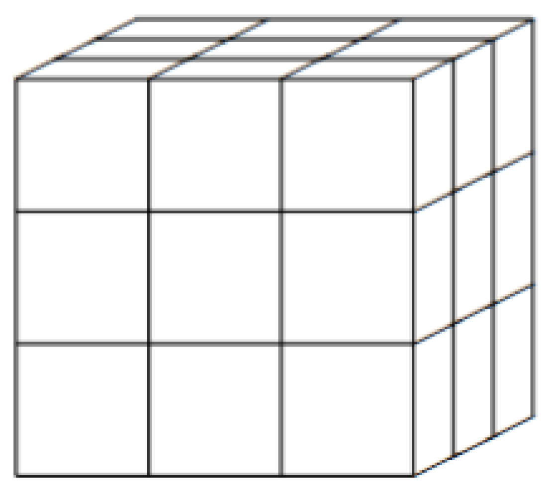
Figure 1 illustrates a subdivision with
. Our integral can then be written as the double sum:
over
terms, integrals over pairs of subcubes:
Results obtained from the subdivision and numerical estimates are given in
Appendix A.
2.3. Removing the Singular Terms
One notes that the double sum (
15) consists of terms for which
, i.e., double integrals over coinciding subcubes, plus terms with
. This means that we can write (
15) as:
where the terms with all three indices the same,
, are excluded in the double sum.
The first sum over coinciding subcubes consists of integrals that are all identical and equal to:
From Equation (
17), one thus obtains:
Apart from being over a smaller cube, the integral
is essentially like the original integral. In fact one easily finds the scaling property:
Using this Equation (
19) becomes:
Solving for , we thus finally have that:
Theorem 1. The original integral (10) with its singularity can be expressed as a sum of integrals without (interior) singularities i.e., without self-interacting subcubes. 3. Coulomb Energy for Electrons
in a Cube
Here, we give explicit expressions for the Coulomb energy of electrons in a cube; first for delocalized electrons, then for electrons localized in subcubes.
3.1. Coulomb Energy for Delocalized Electrons in a Cube
We now assume that there are
electrons, all with constant charge densities
in the cube of side-length
L. The Coulomb electrostatic repulsion energy is then according to (
4) given by:
where
and
are given by (
6). All terms in the sum are the same so we obtain:
Repeating the calculations in (
5)–(
10) gives:
for the relevant Coulomb energy. If we assume that these
electrons obey quantum mechanics they cannot all be in the same orbital. Every pair of electrons must have different kinetic energies so that the spin-orbitals are orthogonal.
3.2. Coulomb Energy for Electrons Localized in Sub-Cubes
We now assume that the cube (of side-length
L) is subdivided into
subcubes
of side-length
. These subcubes are given by (
14) if the ranges
are replaced by
. We assume that we have one electron in each of these subcubes. The Coulomb energy is then according to (
4):
since the charge density in each subcube is
. Here the prime on the second sum means that terms with
are excluded, as in Equation (
22). The initial factor of one half is there since the double sum includes every pair
twice. This gives:
We now do the coordinate transformation we did in Equations (
5)–(
7) and obtain:
Skipping the primes, this can now be written:
The integrals here are the ones given in (
16), so we find:
Using Equation (
22), we now obtain:
To compare this to (
25), we can write it as:
This is thus our final result for the Coulomb energy of
electrons each with constant charge density in one of the
subcubes. Note that the overall charge density here,
, is the same as in the delocalized case (
25).
4. Coulomb Energy Difference
The calculations above are of course a bit technical, but the result is easy to understand: the Coulomb repulsion energy is lower when the electrons are localized to different regions of space. In the calculation for the localized case, the self-energies of the electrons are excluded, and this is one of the differences in the two cases. The self-energies are also excluded in the delocalized case but since all electrons are in the same charge distribution most terms are in fact similar to self-interactions.
The energy difference between the two cases is according to (
25) and (
32):
so we find:
The last expression should be valid for macroscopic matter where one can assume that .
It is perhaps more illuminating to express this in terms of the density of the electrons involved,
. This gives:
This quantity is seen to increase with electron density and with the volume
of the cube, and we have:
for the energy gain per volume.
The localized states always have lower electrostatic energy simply because in these states, the electrons are better at avoiding each other. For small L-values the delocalized states have lower energy because of kinetic energy and the uncertainty principle.
5. Localizing Electron Pairs
Let us use the above results and calculations to investigate the localization into electron pairs. We then start by doubling the number of delocalized electrons in
Section 3 to
. To keep the density of electrons constant we must then also double the volume
to
, i.e., change
L to:
From Equation (
25), this gives us:
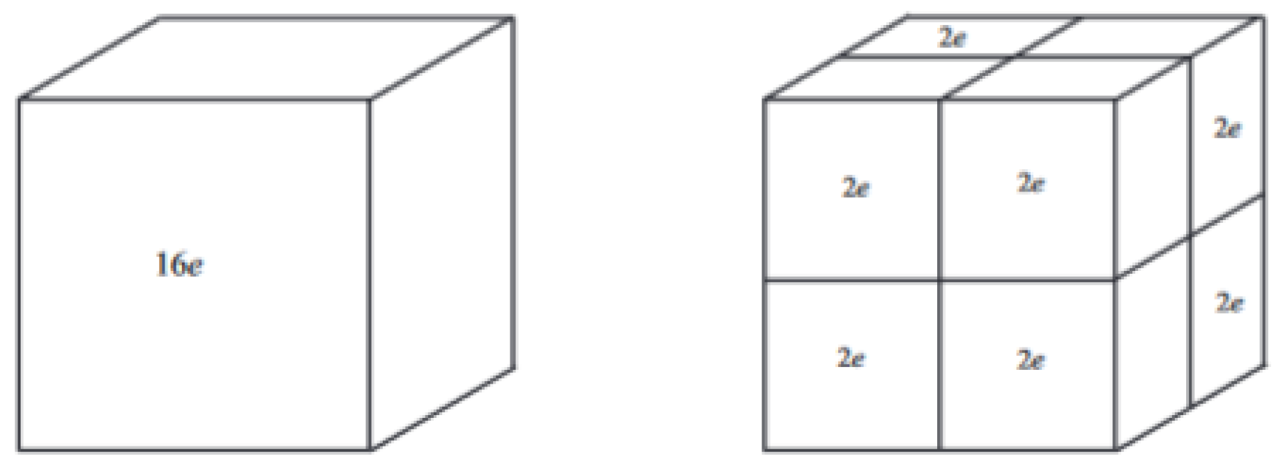
The situation is illustrated for
to the left in
Figure 2.
For the case of two electrons localized in each of the
subcubes, we can use the calculations of
Section 3.2. This situation is illustrated for
to the right in
Figure 2. In Equation (
32), we must now increase the charge
e to
since each subcube now has two electrons. We must also add the repulsion energy within each of the
pairs. This gives an additional contribution to the repulsion energy of:
since the two electrons of charge
e in each of the
subcubes repel each other. These subcubes now have side-length
. So (
32) with
plus (
39) gives us:
or simply
So, this is the repulsion energy when N electron pairs are localized to the subcubes of side-length .
The energy difference between (
38) and (
41) is now:
i.e.,
Comparing this with (
34) we obtain:
so the energy reduction for pairs (maintaining the same overall electron density) is roughly 60% larger. This result is natural since electron pairs repel each other four times more than electrons. This fact together with the Pauli principle makes electron pairing in metals natural, without assuming an attractive force.
To obtain the pair localization energy gain per volume, we start from (
43) and find:
Comparing this to Equation (
36), we see that the localization energy gain for pairs per volume,
, is twice as big as for that of single electrons.
6. The Binding Energy of Pairs
Consider an electron delocalized in a cube of side-length
L with a constant positive charge density of
. The Coulomb binding (or attractive) energy is then:
according to Equation (
9).
Now, double the volume by changing
L to
. Assuming constant charge density the total positive charge in volume now becomes
. To maintain zero net charge density, we assume that there are two electrons delocalized in this cube of volume
. The total Coulomb energy of this system is:
Comparing (
47) with (
46), we see that the pair binding energy is significantly larger than that for a single electron, even when both the electron–electron repulsion and the larger length scale are taken into account. Here, one can object that this is a trivial consequence of the fact that the Coulomb interaction is quadratic in the charges and that the effect is even bigger if triples of electrons are considered. In some sense this is true but the reason to focus on pairs is that because of the Pauli principle one can have one or two electrons in a given spatial state, but not more.
From the above findings, the Cooper pairs in superconductors may in fact be caused by the same mechanism that produce Lewis pairs in quantum chemistry. These pairs were pointed out by Gilbert N. Lewis in 1916 [
34].
7. Conclusions
The Coulomb interaction energy of two constant charge distributions in a cube was written in terms of interactions between subcubes. Considering the constant charge distributions as superpositions of distributions in subcubes, we find the difference between the overall Coulomb interaction and its value without self-interactions within the subcubes. This is of relevance to electron charge distributions since electrons do not self-interact. We thus find exact results on the Coulomb energy gain due to localization of electrons or electron pairs. Within our model, we thus find the Coulomb energy difference between a free electron Fermi gas of delocalized electrons and a Wigner crystal of localized electrons.
Author Contributions
Conceptualization, H.E. Writing—review and editing, J.C.-E.S., H.E. All authors have read and agreed to the published version of the manuscript.
Funding
This research received no external funding.
Institutional Review Board Statement
Not applicable.
Informed Consent Statement
Not applicable.
Data Availability Statement
Not applicable.
Acknowledgments
H.E. is grateful to Zak Seidov for correspondence and to Arne B. Nordmark for discussions.
Conflicts of Interest
The authors declare no conflict of interest.
Appendix A. Subcube Division: Exact Results and Numerical Estimates for
Here we evaluate numerically
of the expression (
22) by taking as much advantage as possible of index symmetries. Each partial integral can be written as:
Denoting
on account of (
20), we have:
Among the
terms (having already precluded the singular terms), there are still many repetitions that can be avoided. In fact, we can write:
To unravel the expression, we first note that the factor
comes from the fact that there are two similar sums of
different varieties, the factor
in front of the double sum is due to four similar sums, each with
varieties, and the factor 8 from the number of similar sums. The first sum contains
terms, the double sum contains
terms, and the triple sum
terms. Taken together, the number of terms is:
as it should.
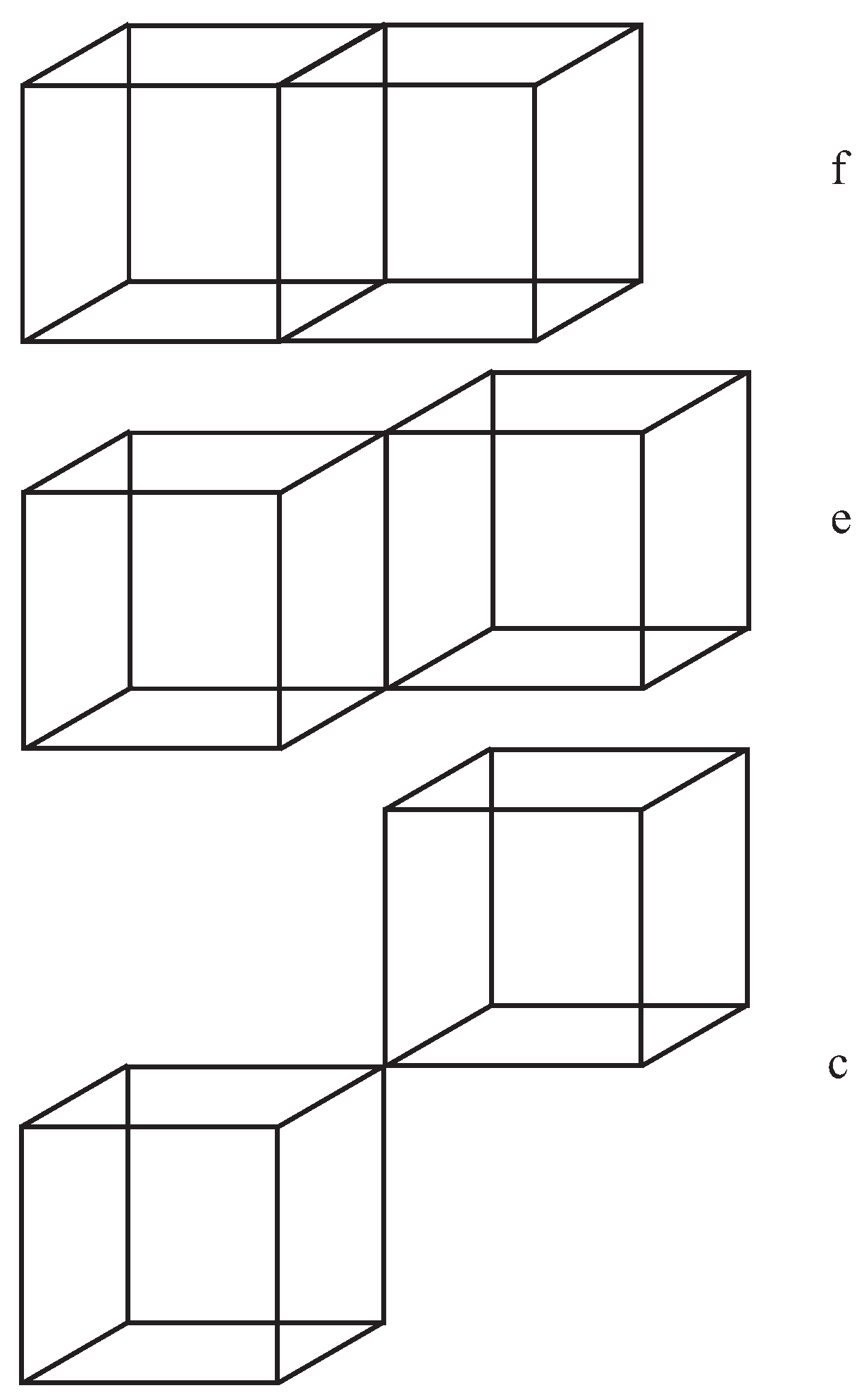
It may be of interest to evaluate the few first cases exactly: for
, illustrated to the right in
Figure 2, Equation (
A3) gives:
using the notation
for the integrals describing interaction between subcubes sharing a face, edge, and vertex (corner), respectively, see
Figure A1. Using (
A1) we find that:
or approximately 1.899556871.
Figure A1.
This figure illustrates three cases of touching cubes for which integrand is singular on a face, an edge, and a corner (vertex), respectively.
Figure A1.
This figure illustrates three cases of touching cubes for which integrand is singular on a face, an edge, and a corner (vertex), respectively.
For
, illustrated in
Figure 1, the number of terms grows significantly. Equation (
A3) gives:
employing the notation
Here (
A1) with
was used. Thus, we find that
which is approximately 1.8907486597. In view of the exact value (
13) the precision is satisfactory. The relative error is approximately
. However in comparison to the expression for
(
A7), which represents a relative error of
, the improvement is unimpressive.
Finally, we note that by means of the Equations (
A5) and (
A8) one can eliminate
, which is singular on a contact surface, and obtain:
which gives
with a relative error of only
.
References
- Madelung, E. Das elektrische Feld in systemen von regelmässig angeordneten Punktladungen. Phys. Z. 1918, 19, 524–532. [Google Scholar]
- Essén, H.; Nordmark, A.B. Some results on the electrostatic energy of ionic crystals. Can. J. Chem. 1996, 74, 885–891. [Google Scholar] [CrossRef]
- Essén, H. The effective shell charge of electrons on a sphere: A discussion of Hund’s rules, negative ions and the chemical bond. Theor. Chim. Acta 1983, 63, 365–376. [Google Scholar] [CrossRef]
- Wigner, E. On the interaction of electrons in metals. Phys. Rev. 1934, 46, 1002–1011. [Google Scholar] [CrossRef]
- Wigner, E. Effects of the electron interaction on the energy levels of electrons in metals. Trans. Faraday Soc. 1938, 34, 678–685. [Google Scholar] [CrossRef]
- Ceperley, D.M.; Alder, B.J. Ground state of the electron gas by a stochastic method. Phys. Rev. Lett. 1980, 45, 566–569. [Google Scholar] [CrossRef] [Green Version]
- Trail, J.R.; Towler, M.D.; Needs, R.J. Unrestricted Hartree-Fock theory of Wigner crystals. Phys. Rev. B 2003, 68, 045107. [Google Scholar] [CrossRef] [Green Version]
- Drummond, N.D.; Radnai, Z.; Trail, J.R.; Towler, M.D.; Needs, R.J. Diffusion quantum monte carlo study of three-dimensional Wigner crystals. Phys. Rev. B 2004, 69, 085116. [Google Scholar] [CrossRef] [Green Version]
- Mott, N.F.; Jones, H. The Theory of the Properites of Metals and Alloys; Dover: New York, NY, USA, 1958. [Google Scholar]
- Seitz, F. The Modern Theory of Solids; McGraw-Hill: New York, NY, USA, 1940. [Google Scholar]
- McWeeny, R.; Sutcliffe, B.T. Methods of Molecular Quantum Mechanics; Academic Press: New York, NY, USA, 1969. [Google Scholar]
- Chalvet, O.; Daudel, R.; Diner, S.; Malrieu, J.P. (Eds.) Localization and Delocalization in Quantum Chemistry—Volume I: Atoms and Molecules in the Ground State; Springer: Berlin, Germany, 1975. [Google Scholar]
- Madelung, O. Introduction to Solid State Theory; Springer: Berlin, Germany, 1978. [Google Scholar]
- Bloch, F. Über die Quantenmechanik der Elektronen in Kristallgittern. Z. Phys. 1929, 52, 555–600. [Google Scholar] [CrossRef]
- Wannier, G.H. The structure of electronic excitation levels in insulating crystals. Phys. Rev. 1937, 52, 191–197. [Google Scholar] [CrossRef]
- Burdett, J.K. From bonds to bands and molecules to solids. Prog. Solid State Chem. 1984, 15, 173–255. [Google Scholar] [CrossRef]
- Hoffmann, R. Solids and Surfaces—A Chemist’s View of Bonding in Extended Structures; VCH: New York, NY, USA, 1988. [Google Scholar]
- Baranov, A.; Kohout, M. Electron localization and delocalization indices for solids. J. Comput. Chem. 2011, 32, 2064–2076. [Google Scholar] [CrossRef] [PubMed]
- Otero-de-la Roza, A.; Pendas, A.M.; Johnson, E.R. Quantitative electron delocalization in solids from maximally localized wannier functions. J. Chem. Theory Comput. 2018, 14, 4699–4710. [Google Scholar] [CrossRef] [Green Version]
- de L. Kronig, R. Zur Theorie der Supraleitfähigkeit. Z. Phys. 1932, 78, 744–750. [Google Scholar] [CrossRef]
- de L. Kronig, R. Zur Theorie der Supraleitfähigkeit II. Z. Phys. 1933, 80, 203–216. [Google Scholar] [CrossRef]
- Shih, B.-C.; Zhang, Y.; Zhang, W.; Zhang, P. Screened Coulomb interaction of localized electrons in solids from first principles. Phys. Rev. B 2012, 85, 045132. [Google Scholar] [CrossRef] [Green Version]
- Shih, B.-C.; Abtew, T.A.; Yuan, X.; Zhang, W.; Zhang, P. Screened Coulomb interactions of localized electrons in transition metals and transition-metal oxides. Phys. Rev. B 2012, 86, 165124. [Google Scholar] [CrossRef]
- Lundberg, M.; Siegbahn, P.E.M. Quantifying the effects of the self-interaction error in dft: When do the delocalized states appear? J. Chem. Phys. 2005, 122, 224103. [Google Scholar] [CrossRef]
- Kohout, M. Electron pairs in position space. In The Chemical Bond II. Structure and Bonding; Mingos, D., Ed.; Springer: Cham, Switzerland, 2016; Volume 170, pp. 119–168. [Google Scholar]
- Essén, H. Electrostatic interaction energies of homogeneous cubic charge distributions. arXiv 2007, arXiv:physics/0701215v1. [Google Scholar]
- Moggia, E.; Bianco, B. Closed form expression for the potential within a face centred cubic ionic crystal. J. Electrost. 2004, 61, 269–280. [Google Scholar] [CrossRef]
- Waldvogel, J. The Newtonian potential of a homogeneous cube. Zeitschr. Angew. Math. Phys. 1976, 27, 867–871. [Google Scholar] [CrossRef]
- Chen, Y.T.; Cook, A. Gravitational Experiments in the Laboratory; Cambridge University Press: Cambridge, UK, 1993. [Google Scholar]
- Hummer, G. Electrostatic potential of a homogeneously charged square and cube in two and three dimensions. J. Electrost. 1996, 36, 285–291. [Google Scholar] [CrossRef]
- Seidov, Z.F.; Skvirsky, P.I. Gravitational potential and energy of homogeneous rectangular parallelepiped. arXiv 2000, arXiv:astro-ph/0002496. [Google Scholar]
- Reitan, D.K.; Higgins, T.J. Calculation of the electrical capacitance of a cube. J. Appl. Phys. 1951, 22, 223–226. [Google Scholar] [CrossRef]
- Hwang, C.-O.; Mascagni, M. Electrical capacitance of the unit cube. J. Appl. Phys. 2004, 95, 3798–3802. [Google Scholar] [CrossRef] [Green Version]
- Lewis, G.N. The atom and the molecule. J. Am. Chem. Soc. 1916, 38, 762–785. [Google Scholar] [CrossRef] [Green Version]
| Publisher’s Note: MDPI stays neutral with regard to jurisdictional claims in published maps and institutional affiliations. |
© 2022 by the authors. Licensee MDPI, Basel, Switzerland. This article is an open access article distributed under the terms and conditions of the Creative Commons Attribution (CC BY) license (https://creativecommons.org/licenses/by/4.0/).


