Hybrid Machine Learning Models for Predicting the Impact of Light Wavelengths on Algal Growth in Freshwater Ecosystems

Abstract

This study examines the influence of light wavelengths on the growth dynamics of five algal genera (Chlorella sp., Volvox sp., Gloeocapsa sp., Microspora sp., and Mougeotia sp.) in freshwater systems, using machine learning to optimize growth models. Natural light yielded the highest algal proliferation, increasing the total count from 90 to 1390 cells/mL in 30 days. Filtered wavelengths showed that blue light most effective (840 cells/mL), followed by red (490 cells/mL) and yellow (200 cells/mL), while green light minimally impacted growth (160 cells/mL). Genera-specific responses revealed that Gloeocapsa sp. and Mougeotia sp. thrived the most under blue light (240 and 750 cells/mL, respectively), with red and blue wavelengths generally enhancing growth across genera. Machine learning models achieved high accuracy (R² > 0.96 for total growth and R² > 0.8 for genera-specific and wavelength-based models), refining growth kinetics. These results suggest that spectral manipulation limiting blue/red wavelengths in water treatment to curb blooms while leveraging natural light for biofuel cultivation could optimize algal management. The integration of empirical data with machine learning offers a robust framework for predictive modeling in algal research and industrial applications.

1. Introduction

Algae, ranging from unicellular microalgae to multicellular macroalgae, contribute to approximately 40% of global photosynthesis and are key primary producers in aquatic ecosystems [1,2]. Predominantly eukaryotic (except cyanobacteria), they drive nutrient cycling, biodiversity, and energy flow in diverse aquatic environments [3]. Light availability is a major determinant of algal productivity and ecosystem dynamics [4]. Beyond their ecological roles, algae are increasingly being studied in applied contexts, including biotechnology, climate research, and sustainable development.

Algae are widely used in biofuel production, food, pharmaceuticals, and environmental applications due to their high biomass yield [5] and rich biochemical content [6,7]. In water treatment, they aid in nutrient removal, supporting both wastewater and drinking water processes [8,9]. Integrated systems, like the pulsator unit, combine coagulation, flocculation, and clarification, offering space-efficient solutions for algae removal despite higher energy use [10]. Algae may enhance such systems by reducing their chemical demand. They also contribute to carbon sequestration, thereby reinforcing their role in climate mitigation [11]. However, the influence of spectrally filtered natural light on algal productivity and physiology remains underexplored, limiting its optimization in both ecological and engineered systems.

Green microalgae, particularly members of the Chlorophyta, are abundant in freshwater ecosystems and play critical roles in ecological balance and water quality [12]. Among these, Chlorella sp., Volvox sp., Gloeocapsa sp., Microspora sp., and Mougeotia sp. are frequently encountered and were selected for this study due to their ecological importance, bioindicator potential, and biotechnological relevance [13,14,15]. These genera contribute to primary production, nutrient cycling, and pollutant sensitivity, making them valuable for environmental monitoring and applied research [15,16,17]. Their presence across various trophic conditions also offers insight into freshwater ecosystem dynamics and aids in assessing anthropogenic impacts on aquatic habitats.

Natural light comprises a spectrum of wavelengths, including ultraviolet, visible, and infrared light, each of which plays a distinct role in algal photosynthesis [18,19]. Blue (400–500 nm) and red (600–700 nm) wavelengths are critical for photosynthetic efficiency due to chlorophyll absorption, although their availability in aquatic systems is modified by turbidity, Dissolved Organic carbon (DOC), and watercolor [20]. This spectral filtering influences algal community composition and growth rates as light penetrates through the water column, and its intensity and spectral composition are altered due to interactions with suspended particles, dissolved organic matter, and phytoplankton. This spectral filtering not only attenuates certain wavelengths but also shifts their dominance, thereby influencing the algal community composition and growth rates [21].

Most studies on algal photophysiology have focused on isolated wavelengths of artificial light under controlled conditions. While informative, these approaches lack environmental realism. Spectrally filtered natural light, which more accurately reflects in situ aquatic conditions, remains understudied [22,23]. This study examines the effects of filtered natural light on freshwater green algae, addressing a key gap in understanding algal responses under ecologically relevant conditions. Insights into the effects of natural light spectra on growth and biochemical traits are vital for managing aquatic ecosystems and optimizing algal cultivation for industrial applications [24].

Previous findings have indicated that blue light enhances chlorophyll production and photosynthetic efficiency, while red light promotes carotenoid synthesis [19,25]. However, the influence of naturally filtered light on these responses remains poorly characterized, making this investigation both novel and applicable to ecological and biotechnological contexts.

Traditional kinetic models, like Monod or Droop, often fail to capture the nonlinear, transient dynamics of algal growth, especially under low nutrient uptake [26]. In contrast, machine learning (ML) approaches, such as artificial neural networks, support vector regression, and LSTM networks, offer improved accuracy by learning complex patterns from data [27]. Hybrid models that combine mechanistic and ML techniques [28] further enhance prediction and interpretability [29]. However, their application under filtered natural light remains limited despite the spectral variability introduced by such conditions. ML’s ability to integrate real-time sensor data also supports the adaptive monitoring of algal blooms in dynamic aquatic environments [30].

This study integrates spectral light filtering with machine learning to model algal growth under environmentally realistic conditions. By bridging empirical ecology and predictive modeling, this study aims to improve the understanding of light-driven algal dynamics. These findings have practical implications for optimizing biofuel yields and managing harmful algal blooms.

2. Materials and Methods

To mimic natural conditions, initial water samples were collected from the “Methetilla Oya” stream in the Badulla District of Sri Lanka. Sampling was conducted in September 2023 at ten random locations (

Table 1. Sampling locations.

Sample Number	Location
Sample 1	6°48′57.59″ N, 80°55′44.14″ E
Sample 2	6°48′56.48″ N, 80°55′43.21″ E
Sample 3	6°48′55.87″ N, 80°55′41.48″ E
Sample 4	6°48′53.78″ N, 80°55′40.16″ E
Sample 5	6°48′52.29″ N, 80°55′38.87″ E
Sample 6	6°48′50.17″ N, 80°55′37.65″ E
Sample 7	6°48′46.84″ N, 80°55′35.47″ E
Sample 8	6°48′43.40″ N, 80°55′28.21″ E
Sample 9	6°48′33.86″ N, 80°55′27.94″ E
Sample 10	6°48′29.14″ N, 80°55′21.89″ E

), and the collected samples were combined to form a composite sample. The composite samples were subjected to several conditions for a period of one month, from September to October 2023, to observe the effects of varying light spectra on water quality and algal growth.

For the experiments, the composite sample was evenly distributed into 15 sterilized transparent glass bottles of 3 L capacity without closing their lids but covered with a plankton net (0.3 mm openings) to facilitate atmospheric O₂ and CO₂ dissociation with the liquid. Four groups of samples were covered with different colored cellophane papers (Local Markt, Kandy City, Sri Lanka) to selectively filter specific light wavelengths from natural sunlight. The treatments included Red (wavelengths of 620–750 nm), Blue (450–495 nm), Green (495–570 nm), and Yellow (570–590 nm). The colored cellophane color distribution in the red (600–700 nm), green (500–600 nm), and blue (400–500 nm) filters was measured by scanning with a UV–visible spectrophotometer (HITACHI U-1900, Tokyo, Japan) sourced from Uva Wellassa University of Sri Lanka. One group was kept uncovered with cellophane and served as the control. Afterwards, all the samples were kept under a shed with a roof made out of transparent glass (with proper ventilation) where direct sunlight fell on the samples for a one-month period. Sri Lanka’s annual average photoperiod of 860 to 1150 µmol photons m⁻² s⁻¹ was exposed for approximately 12 h [31]. The samples were collected under the same photoperiod and exposure conditions, ensuring that any observed differences in algal growth could be reasonably attributed to spectral differences rather than intensity alone. During the experimental period, the maximum and minimum temperatures per day were recorded.

Each day, 100 mL of sample was collected from the control treatment bottles for green microalgae counting and identification. Prior to sampling, the jars were agitated to ensure sample homogeneity. An equal volume (100 mL) of distilled water was then added to replace the removed sample, maintaining a consistent concentration and cell density. The samples were preserved with Lugol’s iodine solution for 48 h to facilitate total cell counting (in triplicate) and recording of live microalgae cell counts (single count by mixing three replicate samples). Using a hemocytometer (Marienfeld GmbH & Co., Lauda-Königshofen, Germany) and a light microscope (Labomed CXL Trinocular, Capelle aan den IJssel, The Netherlands) equipped with an online attached camera, green algae genera were identified and counted. Subsequently, at 2-day intervals, 100 mL samples were collected from each treatment and mixed within the replicates of each treatment, treated with Lugol’s solution, and processed for microalgal cell identification and enumeration. Live images displayed on a connected PC were used to ensure precise and accurate identification. In addition to cell counts, key water quality parameters, including pH, total dissolved solids (TDS), and electrical conductivity (EC), were measured using a multiparameter meter (Hanna-HI-98594, Hanna instruments, Bedfordshire, UK) and recorded for all samples throughout the study. Turbidity values of raw water samples were recorded with Velp-TB1 (Velp, Usmate Velate (MB), Italy) and 2100Q (Hach, Loveland, CO, USA) turbidity meters.

Modeling of Growth Kinetics of Algae Cells with Machine Learning

Mathematical modeling was conducted using Python Code, version 3.13.4 (Appendix A) to predict algal growth kinetics under various wavelengths of light, aiming to identify optimal conditions for large-scale harvesting. The primary dataset, which included daily cell counts across different genera, was loaded from a CSV file and preprocessed for further analysis.

A range of well-established empirical mathematical models were applied to the data, including linear, exponential, logarithmic, polynomial, power, Gaussian, sigmoid, rational, and inverse polynomial functions. These models were first fitted to the cell count data using the curve-fitting function from SciPy, a widely used method for nonlinear curve fitting [32]. Initial parameter estimates were carefully selected based on the characteristics of each model to avoid issues such as taking the logarithm of non-positive values or numerical instability. In addition to classical curve fitting, we employed machine learning models to enhance the prediction accuracy of the established mathematical models. Specifically, Random Forest Regressor, Gradient Boosting Regressor, and Support Vector Regression (SVR) were utilized to optimize the empirical mathematical model with the best fit at the initial stage. These machine-learning algorithms are recognized for their ability to handle complex nonlinear relationships within biological datasets [33,34]. The dataset was divided into training (80%) and testing (20%) sets, with cross-validation techniques applied to assess the generalization performance of the models. Cross-validation was performed by splitting the training set into multiple smaller subsets (folds). For each fold, the model was trained on a subset of the data and tested on the remaining portion to ensure that the model’s performance was evaluated across different data splits. This process provided a more reliable estimate of how the models would perform on unseen data, minimizing the risk of overfitting [35]

Feature importance was also analyzed to determine which factors most influenced algal growth predictions. For the Random Forest and Gradient Boosting models, enhanced mathematical models, which inherently provide feature importance scores, were used to identify the key predictors that had the greatest impact on the model performance. This analysis highlighted the most critical environmental or experimental variables contributing to algal growth, offering insights into the conditions that most affect growth patterns.

For the SVR model, the input features were standardized using a Standard Scaler to optimize performance, as machine learning models are sensitive to the scale of the input data [36]. Performance metrics such as R², Mean Squared Error (MSE), and others were used to evaluate each model’s predictive ability during cross-validation, ensuring that the models could generalize well to new, unseen data.

Visualization techniques were incorporated into the code to plot the observed growth trends alongside the best-fitting models, displaying the corresponding equations and statistical values. The code was executed on the Google Colab open-source platform. The total predicted cell counts were aggregated by summing the outputs of the best-fit models for comparative analysis against the observed data. The results provide a detailed breakdown of the best-fitting model for each genus, graphical representations of growth curves, total biomass predictions, and a summary table of model equations, parameters, and evaluation metrics. This comprehensive approach, which includes cross-validation for model reliability and feature importance analysis, enhances our understanding of algal growth responses to light variations, contributing to the development of more effective strategies for biofuel production under natural conditions.

3. Results and Discussion

3.1. Algae Type Identified

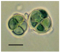
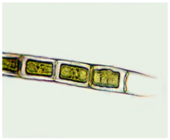
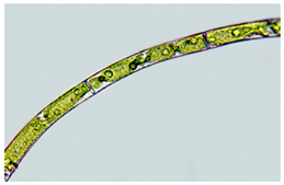
During the initial observation, five major algae genera available in the water were identified and are described in

Table 2. Major algae genera observed in the study.

Algae Type	Image	Specific Characters	References
Chlorella sp.		The microalgae genus Chlorella, particularly genera like Chlorella vulgaris and formerly Chlorella pyrenoidosa, is known for its abundance of chlorophyll a and b, which enables efficient photosynthesis. These algae typically grow spontaneously in freshwater environments.	[37]
Volvox sp.		Volvox is a green algae which comprises about 20 genera, such as V. aureus, V. carteri (V. nagariensis), V. globator, V. dissipatrix, and V. tertius. Volvox group favorably lived in a wide range of water bodies, including deep ponds, lagoons, and especially nitrogenous contaminated water bodies. It is responsible for greenish water in bodies.	[38,39]
Gloeoscapsa sp.		Gleoscapsa sp. Belongs to the Chroococcaceae family and forms an extensive gelatinous colony and red, brown or orange gelatinous globs on substrates in or near water.	[40,41,42]
Microspora sp.		Microspora is a type of green algae belonging to the unbranched, filamentous chlorophytes. Its cell walls are made up of overlapping H-shaped sections, which can vary in thickness. Each individual cell contains a single, deep green, net-like chloroplast. A red pigment is often visible within a lens-shaped cavity located between the cells. Microspora is typically found in streams and rivers with moderate to good water quality, thriving in environments where conditions are relatively clean and stable.	[43,44]
Mugeotia sp.		Mugeotia genus green algae consists of more than 200 genera, which are habitat in freshwater, including lakes, ponds, rivers and sub-areal conditions. At the same time, this genre consists of filamentous form.	[45]

at an average maximum and minimum temperature range of 26.5–18.9 °C. The identified genera were Chlorella sp., Volvox sp., Gloeoscap sp., and Microspora sp. And Mugeotia sp. In addition, there were a few other spices with very low quantities that were not characterized.

3.2. Algae Count (Cells/mL) Under Different Wavelength Light

Algae development under various colored cellophane treatments from 1 September to 1 October 2024, showed distinct patterns influenced by light wavelength (Figure 1). The measured light intensity reductions through filtering by red, blue, green, and yellow cellophane were 301, 473, 559, and 344 µmol photons m⁻² s⁻¹, respectively, at a light level of 867 µmol m⁻² s⁻¹. The control samples under unfiltered sunlight displayed steady growth, increasing from 90 to 1390 cells/mL. The algae under the red and yellow filters reached 490 and 200 cells/mL, respectively, indicating moderate growth. The green cellophane had a minimal effect, with counts rising only to 160 cells/mL. In contrast, blue cellophane was the most effective, increasing the cell count to 840 cells/mL, highlighting its support for algal proliferation. To assess statistical differences among the five groups (Blank, Red, Yellow, Green, and Blue) across 31 time points, the study included (a) descriptive statistics, (b) one-way ANOVA, and (c) post hoc analysis using Tukey HSD, with results summarized in Table 2.

According to

Table 3. Statistical analysis of the total algae cell counts over a month period.

(a) Descriptive Statistics
Group	Mean	Standard Deviation	Minimum	Maximum
Blank	580	416.82	90	1390
Red	340	145.55	90	490
Yellow	155.16	34.6	90	200
Green	117.42	23.19	90	160
Blue	635	238.7	90	840
(b) One-Way ANOVA
Source	Sum of Squares	df	Mean Square	F	p-Value
Group	1.13 × 106	4	283,498.7	17.79	<0.0001
Residual	2.37 × 106	150	15,785.3
(c) Post Hoc Analysis (Tukey HSD)
Comparison	Mean Difference	95% CI (Lower, Upper)	p-Value	Significant?
Blank vs. Red	−210	[−354.2, −65.8]	0.0009	Yes
Blank vs. Yellow	−343.5	[−487.8, −199.3]	<0.0001	Yes
Blank vs. Green	−373.2	[−517.5, −229.0]	<0.0001	Yes
Blank vs. Blue	−152.6	[−296.8, −8.3]	0.0324	Yes
Red vs. Yellow	−133.5	[−277.8, 10.7]	0.0839	No
Red vs. Green	163.2	[19.0, 307.5]	0.0179	Yes
Red vs. Blue	−57.4	[−201.7, 86.8]	0.8067	No
Yellow vs. Green	29.7	[−114.6, 173.9]	0.9795	No
Yellow vs. Blue	−191	[−335.2, −46.7]	0.0032	Yes
Green vs. Blue	−220.6	[−364.9, −76.4]	0.0004	Yes

a, the Blue and Blank groups showed the highest mean responses, while the Green group showed the lowest. The Blank group also had the greatest variability, suggesting an increasing response over time. The ANOVA results [F(4150) = 17.79, p < 0.0001] in Table 3b indicate significant differences among group means. Pairwise comparisons in Table 3c show that the Blank group differed notably from all other groups, suggesting a distinct control effect. The Green group had consistently lower values that were significantly different from those of the Blue and Red groups, which themselves showed no significant difference, indicating similar response levels.

These findings confirm that unfiltered light supports the highest algal growth, likely due to the higher total light availability and broader spectral coverage. In contrast, spectral filters may limit the critical wavelengths and reduce the overall light intensity, thereby constraining growth. Among the filtered wavelengths, blue cellophane light was the most effective, promoting rapid growth, especially in the latter half of the study, while green was the least effective. Red and yellow supported moderate growth, exceeding control levels but not significantly different from blue.

Our results align with those of previous studies, including those by Maltsev et al. (2021) and de Mooij et al. (2016) [20,46], which highlighted the effectiveness of blue and red cellophane-filtered light in boosting microalgal biomass. Shankar et al. (2022) also support this, noting that microalgae possess photoreceptors responsive to these wavelengths, enhancing growth [47]. The Yellow group showed intermediate responses that were not statistically different from those of the Red or Green groups, suggesting a moderate effect. In contrast, the Green group had the lowest responses and differed significantly from most groups, except for the Yellow group, indicating a minimal impact. These findings reinforce the potential of targeted wavelengths to optimize algal cultivation in natural environments.

Our results demonstrate that light wavelength can be strategically used to manage algal growth in water treatment settings. Yellow and green cellophane filters resulted in minimal growth, making them suitable for limiting algae. In contrast, blue and red filters promote growth and can be utilized in controlled environments to boost biofuel production: blue for early cultivation and red for maintaining high biomass in later stages. This strategic use of light can maximize the yield for biofuel applications [25,46,47].

3.3. Growth of Different Algae in Different Wavelength Light

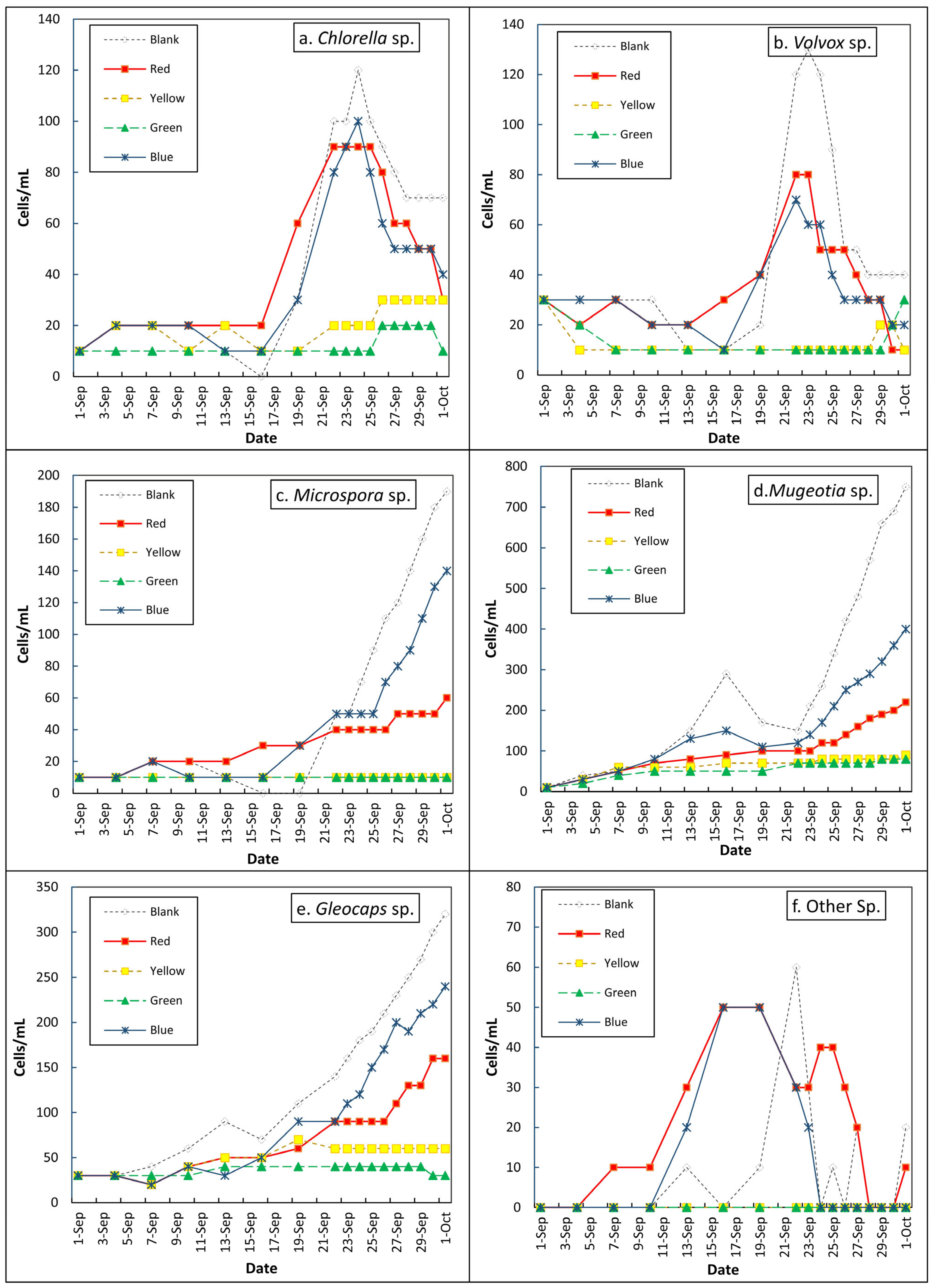
The algae growth patterns under Red, Yellow, Green, Blue, and Blank cellophane filters over a month (Figure 2) offer insights into managing algal proliferation in water treatment and enhancing biofuel production. Green and yellow filters had the lowest impact on all observed genera (Chlorella, Volvox, Microspora, Mougeotia, and Gloeocapsa), with values between 10 and 20 cells/mL (e.g., Chlorella 12.2, Volvox 13.3’ cells/mL), indicating their effectiveness in suppressing growth and minimizing operational issues. In contrast, natural light promoted the highest growth, averaging 68.9 cells/mL for Microspora and 150 cells/mL for Gloeocapsa, with peaks of approximately 750 cells/mL for Mougeotia [22].

Blue cellophane-filtered light supported rapid growth across all species, averaging 42.8 cells/mL for Chlorella and peaking at 240 cells/mL for Gloeocapsa, making it ideal for early biofuel cultivation. Red-filtered light showed moderate, sustained growth, such as 36.1 cells/mL for Volvox and 109.4 cells/mL for Mougeotia, which suited later productivity stages. This highlights the dual importance of blue and red light in biofuel production systems.

These findings support a strategic approach: yellow and green filters can suppress algae in untreated water systems, while blue and red filters can enhance biomass during the pre-treatment or culture phases. For example, before primary treatment, exposing Volvox or Gloeocapsa to blue and red light can boost biomass yield. This integrated approach ensures the efficient regulation of algae growth in water treatment systems and promotes biofuel production, leading to long-term and useful solutions [48].

Compared to natural or blue light, red cellophane-filtered light was less effective for rapid algal growth but supported moderate, sustained development. Therefore, its use in water treatment should be limited or alternated with other methods to disrupt the algal cycle. However, red light can be valuable for biofuel production to maintain productivity following initial blue light cultivation. Yellow and green filters remain effective tools for algae control as they inhibit growth without encouraging proliferation and can be used alone or alongside other strategies.

Figure 2 shows the maximum cell counts (cells/mL) for each genus under various light wavelengths, along with the specific days on which these peaks occurred. Chlorella sp. Genera peaked at 1390 cells/mL on day 31 under red light and 1280 cells/mL on day 30 under blue light. Volvox reached 490 cells/mL on day 31 (red line) and 470 cells/mL on day 30 (blue). Microspora sp. peaked at 340 cells/mL on day 19 under red light and 330 cells/mL under blue light. Mugeotia sp. showed 220 cells/mL under red and 200 cells/mL under blue light on day 31. Gloeocapsa sp. peaked at 320 cells/mL (red) and 300 cells/mL (blue). “Other Genera.” reached 750 cells/mL (red) and 690 cells/mL (blue). These trends confirm that red and blue lights support high cell proliferation, particularly in the later stages.

However, Chlorella sp. and Volvox sp. showed a decline in cell density toward the end, unlike the other genera that maintained steady growth. One likely explanation is nutrient depletion, as both Chlorella and Volvox experienced rapid early growth, potentially exhausting key resources such as nitrogen and phosphorus, which are essential for sustained cell division [49]. Additionally, self-shading effects caused by high cell densities may limit internal light penetration within the culture medium, leading to reduced photosynthetic efficiency and growth inhibition [50]. The accumulation of toxic metabolic byproducts and pH shifts due to prolonged dense cultivation could also contribute to cellular stress and subsequent population decline [51]. Furthermore, the colonial and more complex life cycle of Volvox may involve natural population senescence following the reproductive phase, a phenomenon not observed in other unicellular or filamentous taxa examined [52]. These factors together suggest that the decline in these two species reflects biological limitations rather than the effects of light treatment alone, underscoring species-specific growth dynamics under semi-natural conditions.

3.4. Growth of Different Algae in the Same Wavelength Light

The growth of algal genera under different cellophane-filtered light conditions (Figure 3) provides insights into their responsiveness to specific wavelengths, which is relevant for both water treatment and biofuel production. Under natural light, Gloeocapsa sp. and Mougeotia sp. grew steadily, while Microspora sp. grew more slowly. Volvox sp. and Chlorella sp. showed moderate to low growth, indicating limited responsiveness. Red cellophane-filtered light reduced overall growth but still supported moderate growth (up to 200 cells/mL) in Mougeotia sp., Gloeocapsa sp., Microspora sp. However, Volvox sp. and Chlorella sp. remained consistently low under both natural and red light.

Responses to the yellow, green, and blue filters varied (Figure 3a–e). Yellow light promotes steady growth in Mougeotia sp. and Chlorella sp., while Volvox sp., Microspora sp., and Gloeocapsa sp. show minimal changes, indicating limited adaptation. Green cellophane supports the continued growth of Mougeotia sp., which dominates late in the month. Gloeocapsa sp. grows initially but declines mid-September; other genera remain low. Blue light fosters strong growth in Mougeotia sp. and Gloeocapsa sp. post-mid-September, while the others show a minimal response.

These results have practical applications in water treatment and biofuel systems. The limited growth of Chlorella sp. and Volvox sp. under natural and red light suggests that these wavelengths could suppress their proliferation. Avoiding yellow light could help control Mougeotia sp. and Chlorella sp. in the treatment systems. Conversely, blue light can support the cultivation of Mougeotia sp. and Gloeocapsa sp. for biofuel production due to their high biomass output. Although less effective, red light enables moderate growth in Gloeocapsa sp. and Microspora sp., offering an energy-efficient cultivation option.

The integration of these approaches can help achieve the dual objectives of water treatment and biofuel production. Tailoring cellophane-filtered light conditions can suppress harmful algal blooms and maintain system efficiency in water treatment plants while simultaneously promoting the growth of high-biomass genera for biofuel applications. For example, the use of green cellophane-filtered light to suppress non-dominant genera while encouraging Mougeotia sp. growth aligns with biofuel production goals. These results highlight the potential of light manipulation to optimize genera-specific algal growth, paving the way for sustainable and efficient water treatment and biofuel production systems.

3.5. Application of Machine Learning in Algal Growth Kinetics Modeling

Machine learning models were trained and evaluated using R² scores to assess the prediction accuracy for each genus. The model with the highest coefficient of determination (R²) in the test set was chosen as the best performer. The predictions were plotted against the actual data to visually assess the performance, and the best-fit equation was included in the plot to illustrate the relationship between time and cell count. To understand the total growth trends, predictions for each genus were summed, and an overall R² was calculated to evaluate the combined model accuracy.

This method integrates classical curve fitting with modern machine learning, thereby enhancing the analysis of biological growth. Machine learning captures complex nonlinear trends that traditional models may miss, providing deeper insights into the growth dynamics of different genera over time. By leveraging machine learning, we were able to model complex nonlinear behaviors in the data that traditional approaches might struggle to capture, offering deeper insights into the growth kinetics of various genres.

3.5.1. Growth of Kinetics of Algae Genera Under Natural Light

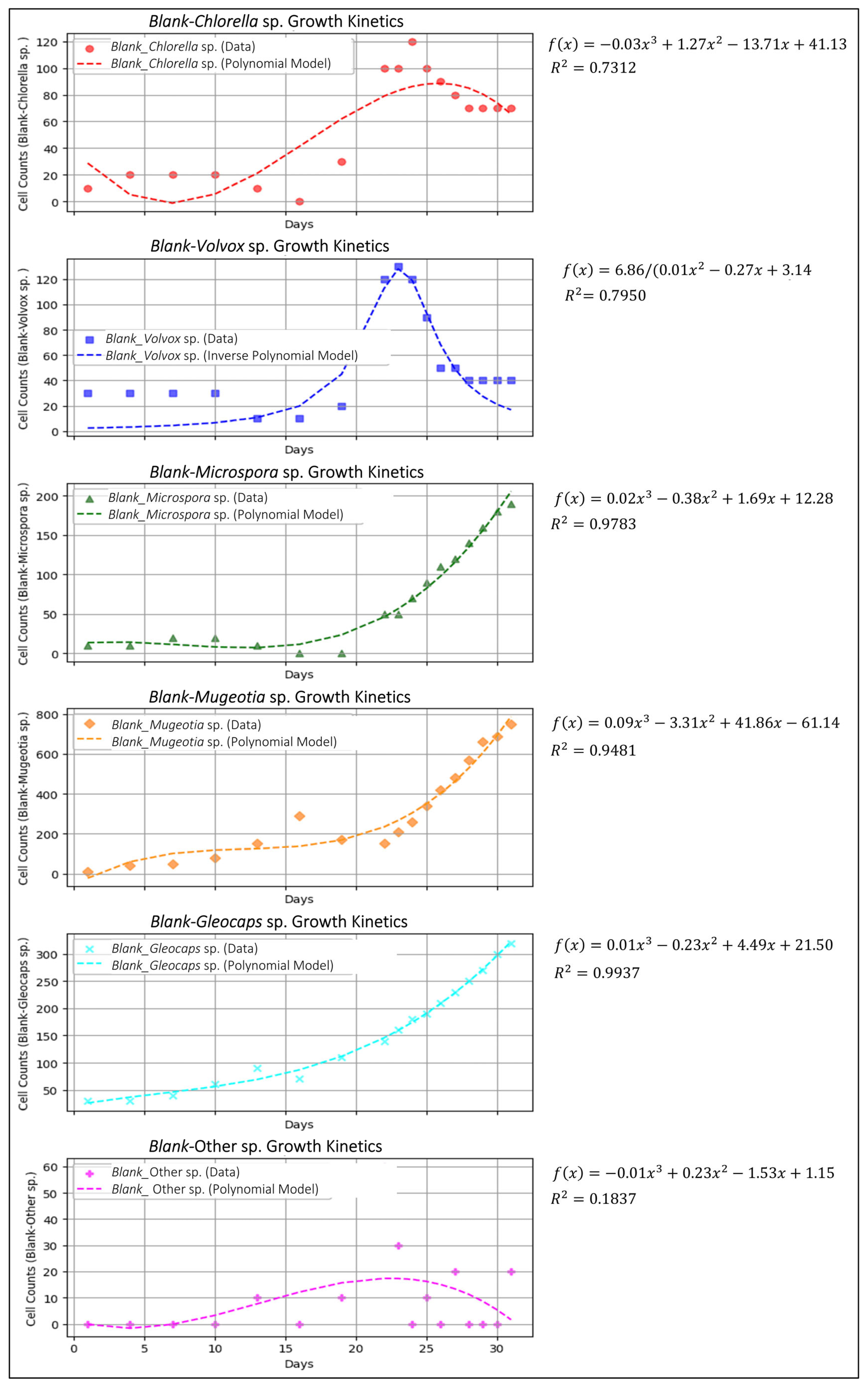
The machine learning models effectively captured the growth kinetics (R² > 0.96; Figure 4, Figure 5 and Figure 6). High accuracy was achieved for Mugeotia (R² = 0.9937), Gloeocapsa (R² = 0.9937), and Microspora (R² = 0.9783), though lower for Chlorella (R² = 0.7312) and Volvox (R² = 0.7950). The hybrid approach combining curve fitting with Random Forest/Gradient Boosting regressors outperformed traditional polynomial models in capturing biological growth patterns [53].

Additionally, biological growth is influenced by numerous factors, such as nutrient availability, environmental conditions, and inter-genera interactions. These multifaceted influences can result in data that simple polynomial models may not explain adequately. By exploring a variety of model architectures and incorporating methods that can adapt to these nonlinear relationships, our analysis aligns more closely with the underlying biological processes. As highlighted by Liu, Huang, et al. (2023), incorporating diverse modeling approaches, including those that account for external environmental factors, can enhance predictive accuracy and provide deeper insights into growth kinetics [53].

Thus, the combination of traditional curve-fitting techniques with machine learning models in our code provides a robust framework for understanding and predicting the growth dynamics of algal genera. This multi-model strategy not only improves model accuracy but also enhances our overall understanding of the complex biological mechanisms involved.

3.5.2. Growth of Kinetics of Total Algae

The best-fit curve shown in Figure 5 represents the total cell count prediction using the sum of individual algae genera growth kinetics fitted functions obtained (Figure 4). The high R² value (0.9941) indicates a strong correlation between the predicted and actual values, suggesting that the model effectively captured the overall growth trend. This strong fit is likely influenced by a genus with machine learning assisted with modified models.

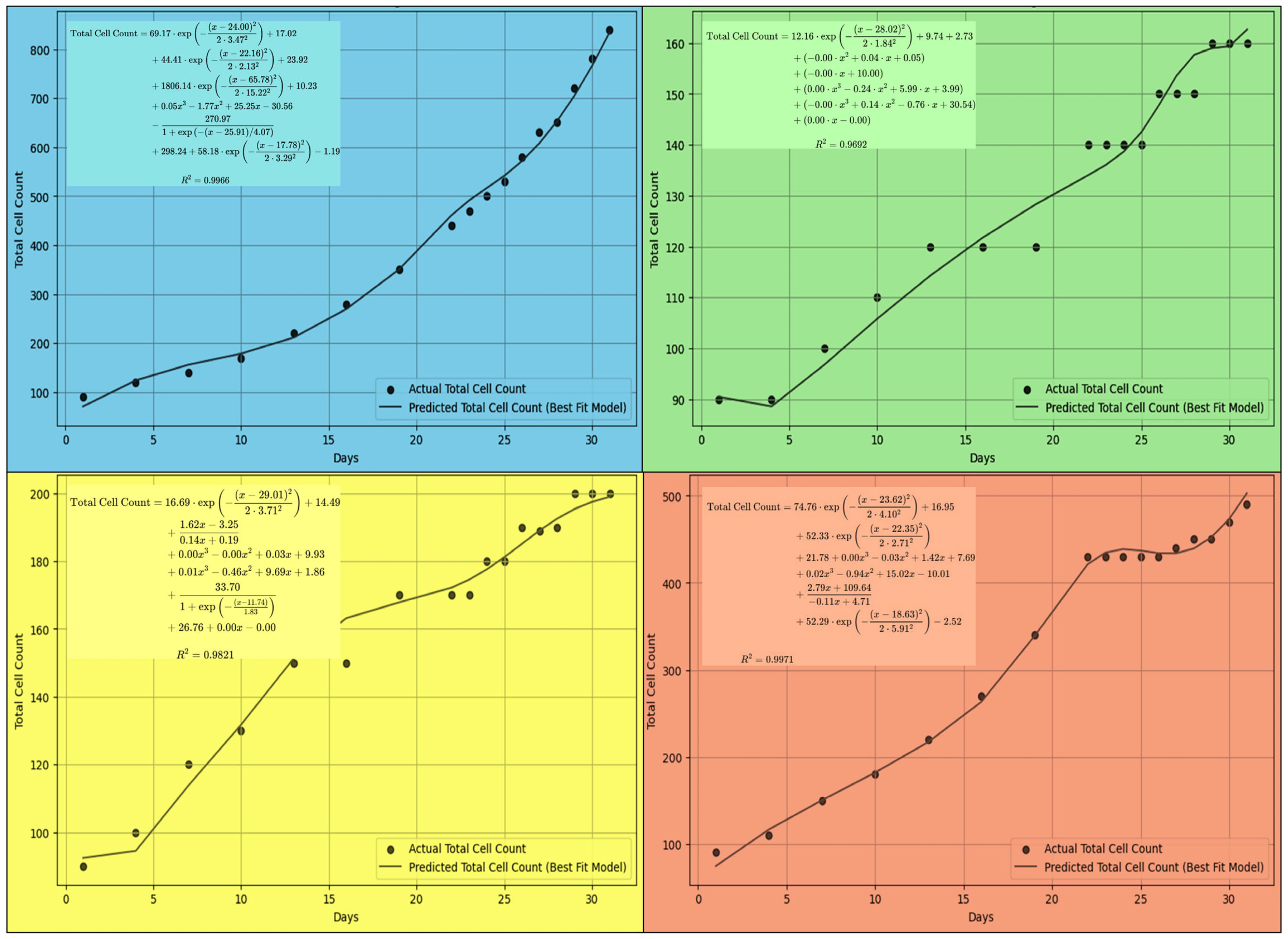
Accordingly, the same machine learning approach was utilized to identify the best-fit curve for algae growth under different wavelengths (Figure 6). Similar to the previous Section 3.5.1 and Section 3.5.2, individual genera’ growth curves were aggregated to model total algal proliferation under specific spectral conditions. This methodology provides valuable insights into forecasting natural growth patterns and optimizing cultivation strategies.

The influence of light wavelength on photosynthetic efficiency directly impacts biomass accumulation and lipid biosynthesis, both of which are critical factors in biofuel generation. The developed predictive models demonstrated distinct growth trends across spectral variations, highlighting the potential for optimizing light conditions to maximize lipid yield. According to the results shown in Figure 6, the high R² values (higher than 0.96) indicate that the machine learning-optimized regression effectively captured the growth dynamics. While the current regression approach provides reliable short-term predictions (30 days), long-term scalability may require re-verification of the proposed model with experimental results. Accordingly, integrating the proposed algorithm with AI-driven bioreactor systems holds promise for optimizing algal growth, ensuring a sustainable and economically viable approach to biofuel manufacturing.

This study demonstrates that different light wavelengths significantly influence algal proliferation, offering practical applications in algae growth monitoring and biofuel production. Unfiltered natural light promoted the highest algal growth, increasing the cell count from 90 to 1390 cells/mL. Among the colored filters, blue light had the most substantial impact, with Gloeocapsa sp. and Mougeotia sp. reaching peak concentrations of 240 and 750 cells/mL, respectively. Red light facilitated moderate but sustained growth, supporting 109.4 cells/mL of Mougeotia sp. and 36.1 cells/mL of Volvox sp., making them suitable for controlled biofuel cultivation. In contrast, yellow and green light filters effectively suppressed algal growth, with genus-specific cell counts ranging from 10 to 20 cells/mL, indicating their potential in algae control strategies.

4. Conclusions

Machine learning models effectively captured the growth kinetics of algae under different wavelengths, with R² values exceeding 0.96, demonstrating the robustness of predictive modeling for optimizing cultivation. However, limitations remain, including potential variations in light intensity and spectral distribution, which may influence the algal responses. Future studies should employ precise light calibration techniques and explore a broader range of wavelengths to refine the predictive accuracies of growth models. Additionally, environmental factors, such as nutrient availability and temperature fluctuations, were not explicitly controlled in this study and should be considered in subsequent research.

For practical applications, the findings suggest that blue and red light can be strategically utilized in photobioreactor designs to enhance biofuel production, while yellow and green light may be integrated into water treatment systems for algal bloom control. Further studies should explore the integration of AI-driven bioreactors for the real-time optimization of algal growth conditions, ensuring efficient and scalable production. Testing a wider range of algal genera, particularly those with high lipid content for biofuel applications, will further validate the effectiveness of spectral light manipulation in sustainable biotechnology.

References

1. Xu, W.; Gao, Z.; Qi, Z.; Qiu, M.; Peng, J.Q.; Shao, R. Effect of Dietary Chlorella on the Growth Performance and Physiological Parameters of Gibel carp, Carassius auratus gibelio. Turk. J. Fish. Aquat. Sci. 2014, 14, 53–57. [Google Scholar] [CrossRef]
2. Metsoviti, M.N.; Papapolymerou, G.; Karapanagiotidis, I.T.; Katsoulas, N. Effect of Light Intensity and Quality on Growth Rate and Composition of Chlorella vulgaris. Plants 2019, 9, 31. [Google Scholar] [CrossRef]
3. Baldrighi, E.; Grall, J.; Quillien, N.; Carriço, R.; Verdon, V.; Zeppilli, D. Meiofauna communities’ response to an anthropogenic pressure: The case study of green macroalgal bloom on sandy beach in Brittany. Estuar. Coast. Shelf Sci. 2019, 227, 106326. [Google Scholar] [CrossRef]
4. Falkowski, P.G.; Raven, J.A. Aquatic Photosynthesis: Second Edition; Princeton University Press: Princeton, NJ, USA, 2007; p. 512. [Google Scholar]
5. Al-Ketife, A.M.D.; Al-Momani, F. Optimizing biofuel production from algae using four-element framework: Insights for maximum economic returns. Energy Rep. 2024, 12, 1254–1268. [Google Scholar] [CrossRef]
6. Thiviya, P.; Gamage, A.; Gama-Arachchige, N.S.; Merah, O.; Madhujith, T. Seaweeds as a Source of Functional Proteins. Phycology 2022, 2, 216–243. [Google Scholar] [CrossRef]
7. Brennan, L.; Owende, P. Biofuels from microalgae—A review of technologies for production, processing, and extractions of biofuels and co-products. Renew. Sustain. Energy Rev. 2010, 14, 557–577. [Google Scholar] [CrossRef]
8. Skouteris, G.; Rodriguez-Garcia, G.; Reinecke, S.F.; Hampel, U. The use of pure oxygen for aeration in aerobic wastewater treatment: A review of its potential and limitations. Bioresour. Technol. 2020, 312, 123595. [Google Scholar] [CrossRef]
9. Al Ketife, A.M.D.; Al Momani, F.; Judd, S.A. bioassimilation and bioaccumulation model for the removal of heavy metals from wastewater using algae: New strategy. Process Saf. Environ. Prot. 2020, 144, 52–64. [Google Scholar] [CrossRef]
10. Tomonori, K.; Ayuri, M.; Yuka, S.; Amarasooriya, A.A.G.D.; Weragoda, S.K. The Comparison of Two Water Treatment Plants operating with different processes in Kandy City, Sri Lanka. J. Ecotechnology Res. 2016, 18, 1–6. [Google Scholar] [CrossRef]
11. Leliaert, F. Green algae: Chlorophyta and streptophyta. Encycl. Microbiol. 2019, 457–468. [Google Scholar] [CrossRef]
12. Ilieva, Y.; Zaharieva, M.M.; Kroumov, A.D.; Najdenski, H. Antimicrobial and Ecological Potential of Chlorellaceae and Scenedesmaceae with a Focus on Wastewater Treatment and Industry. Fermentation 2024, 10, 341. [Google Scholar] [CrossRef]
13. Khalil, S.; Mahnashi, M.H.; Hussain, M.; Zafar, N.; Un-Nisa, W.; Khan, F.S.; Afzal, U.; Shah, G.M.; Niazi, U.M.; Awais, M.; et al. Exploration and determination of algal role as Bioindicator to evaluate water quality–Probing fresh water algae. Saudi J. Biol. Sci. 2021, 28, 5728–5737. [Google Scholar] [CrossRef] [PubMed]
14. Gupta, A.; Singh, A.P.; Singh, V.K.; Singh, P.R.; Jaiswal, J.; Kumari, N.; Upadhye, V.; Singh, S.C.; Sinha, R.P. Natural Sun-Screening Compounds and DNA-Repair Enzymes: Photoprotection and Photoaging. Catalysts 2023, 13, 745. [Google Scholar] [CrossRef]
15. Song, X.; Bo, Y.; Feng, Y.; Tan, Y.; Zhou, C.; Yan, X.; Ruan, R.; Xu, Q.; Cheng, P. Potential applications for multifunctional microalgae in soil improvement. Front. Environ. Sci. 2022, 10, 1035332. [Google Scholar] [CrossRef]
16. Büdel, B.; Friedl, T.; Beyschlag, W. Biology of Algae, Lichens and Bryophytes; Springer Spektrum: Berlin/Heidelberg, Germany, 2024. [Google Scholar] [CrossRef]
17. Li, K.; Ye, Q.; Li, Q.; Xia, R.; Guo, W.; Cheng, J. Effects of the spatial and spectral distribution of red and blue light on Haematococcus pluvialis growth. Algal Res. 2020, 51, 102045. [Google Scholar] [CrossRef]
18. Nwoba, E.G.; Parlevliet, D.A.; Laird, D.W.; Alameh, K.; Moheimani, N.R. Light management technologies for increasing algal photobioreactor efficiency. Algal Res. 2019, 39, 101433. [Google Scholar] [CrossRef]
19. Ramanna, L.; Rawat, I.; Bux, F. Brightening microalgal potential: A study on organic fluorescent dyes to increase photosynthetic active radiation. Algal Res. 2024, 81, 103585. [Google Scholar] [CrossRef]
20. De Mooij, T.; De-Vries, G.; Latsos, C.; Wijffels, R.H.; Janssen, M. Impact of light color on photobioreactor productivity. Algal Res. 2016, 15, 32–42. [Google Scholar] [CrossRef]
21. Thoral, F.; Pinkerton, M.H.; Tait, L.W.; Schiel, D.R. Spectral light quality on the seabed matters for macroalgal community composition at the extremities of light limitation. Limnol. Oceanogr. 2023, 68, 902–916. [Google Scholar] [CrossRef]
22. Baidya, A.; Akter, T.; Islam, M.R.; Shah, A.K.M.A.; Hossain, M.A.; Salam, M.A.; Paul, S.I. Effect of different wavelengths of LED light on the growth, chlorophyll, β-carotene content and proximate composition of Chlorella ellipsoidea. Heliyon 2021, 7, 08525. [Google Scholar] [CrossRef]
23. Yan, C.; Zhang, L.; Luo, X.; Zheng, Z. Effects of various LED light wavelengths and intensities on the performance of purifying synthetic domestic sewage by microalgae at different influent C/N ratios. Ecol. Eng. 2013, 51, 24–32. [Google Scholar] [CrossRef]
24. Foroutan, R.; Esmaeili, H.; Abbasi, M.; Rezakazemi, M.; Mesbah, M. Adsorption behavior of Cu(II) and Co(II) using chemically modified marine algae. Environ. Technol. 2018, 39, 2792–2800. [Google Scholar] [CrossRef] [PubMed]
25. Liu, J.; Van Iersel, M.W. Photosynthetic Physiology of Blue, Green, and Red Light: Light Intensity Effects and Underlying Mechanisms. Front. Plant Sci. 2021, 12, 619987. [Google Scholar] [CrossRef]
26. Wang, H.; Garcia, P.V.; Ahmed, S.; Heggerud, C.M. Mathematical comparison and empirical review of the Monod and Droop forms for resource-based population dynamics. Ecol. Modell. 2022, 466, 109887. [Google Scholar] [CrossRef]
27. Mazzuca Sobczuk, T.; Ao, Y.; Fan, J.; Guo, F.; Li, M.; Li, A.; Shi, Y.; Wei, J. Machine Learning-Based Early Warning of Algal Blooms: A Case Study of Key Environmental Factors in the Anzhaoxin River Basin. Water 2025, 17, 725. [Google Scholar] [CrossRef]
28. Liu, M.; He, J.; Huang, Y.; Tang, T.; Hu, J.; Xiao, X. Algal bloom forecasting with time-frequency analysis: A hybrid deep learning approach. Water Res. 2022, 219, 118591. [Google Scholar] [CrossRef] [PubMed]
29. Schweidtmann, A.M.; Zhang, D.; Von-Stosch, M.A. review and perspective on hybrid modeling methodologies. Digit. Chem. Eng. 2024, 10, 100136. [Google Scholar] [CrossRef]
30. Park, J.; Patel, K.; Lee, W.H. Recent advances in algal bloom detection and prediction technology using machine learning. Sci. Total Environ. 2024, 938, 17354. [Google Scholar] [CrossRef]
31. Renne, P.; George, R.; Marion, B.; Heimiller, D.; Gueymard, C. Solar Resource Assessment for Sri Lanka and Maldives. In National Renewable Energe Laboratory; Department of Energy Laboratory: Golden, CO, USA, 2003. Available online: https://docs.nrel.gov/docs/fy03osti/34645.pdf (accessed on 3 March 2025).
32. Virtanen, P.; Gommers, R.; Oliphant, T.E.; Haberland, M.; Reddy, T.; Cournapeau, D.; Burovski, E.; Peterson, P.; Weckesser, W.; Bright, J.; et al. SciPy 1.0: Fundamental algorithms for scientific computing in Python. Nat. Methods 2020, 17, 261–272. [Google Scholar] [CrossRef]
33. Breiman, L. Random forests. Mach. Learn. 2001, 45, 5–32. [Google Scholar] [CrossRef]
34. Friedman, J.H. Greedy function approximation: A gradient boosting machine. Ann. Stat. 2001, 29, 1189–1232. [Google Scholar] [CrossRef]
35. Kohavi, R. A Study of Cross-Validation and Bootstrap for Accuracy Estimation and Model Selection. Stanford University, Stanford, CA, USA. 1995. Available online: https://www.ijcai.org/Proceedings/95-2/Papers/016.pdf (accessed on 3 January 2025).
36. Pedregosa, F.; Michel, V.; Grisel, O.; Blondel, M.; Prettenhofer, P.; Weiss, R.; Vanderplas, J.; Cournapeau, D.; Pedregosa, F.; Varoquaux, G.; et al. Machine Learning in Python. J. Mach. Learn. Res. 2011, 12, 2825–2830. [Google Scholar] [CrossRef]
37. Toniolo, C.; Nicoletti, M. Chapter 43-Quality control of microalgae-derived products. In Handbook of Food and Feed from Microalgae; Jacob-Lopes, E., Queiroz, M.I., Maroneze, M.M., Zepka, L.Q., Eds.; Academic Press: Cambridge, MA, USA, 2023; pp. 567–575. ISBN 9780323991964. [Google Scholar] [CrossRef]
38. El-Bawab, F. Chapter 3-Phylum Protozoa. In Invertebrate Embryology and Reproduction, El-Bawab, F., Ed.; Academic Press: Cambridge, MA, USA, 2020; pp. 68–102. ISBN 9780128141144. [Google Scholar] [CrossRef]
39. Matt, G.; Umen, J. Volvox: A simple algal model for embryogenesis, morphogenesis and cellular differentiation. Dev. Biol. 2016, 419, 99–113. [Google Scholar] [CrossRef] [PubMed]
40. Macedo, M.; Miller, A.; Dionísio, A.; Saiz-Jimenez, C. Biodiversity of cyanobacteria and green algae on monuments in the Mediterranean Basin: An overview. Microbiology 2009, 155, 3476–3490. [Google Scholar] [CrossRef] [PubMed]
41. Serediak, N.; Huynh, M. Algae Identification-Lab Guide: Accompanying Manual to the Algae Identification Field Guide; Agriculture and Agri-Food Canada: Ottawa, ON, Canada, 2011; pp. 1–40. [Google Scholar]
42. Komárek, J. 3-Coccoid And Colonial Cyanobacteria. In Freshwater Algae of North America; Wehr, J.D., Sheath, R.G., Eds.; Academic Press: Burlington, VT, USA, 2003; pp. 59–116. [Google Scholar]
43. Lokhorst, G.M.; Star, W. The flagellar apparatus structure in Microspora (Chlorophyceae) confirms a close evolutionary relationship with unicellular green algae. Plant Syst. Evol. 1999, 217, 11–30. [Google Scholar] [CrossRef]
44. Available online: https://www.landcareresearch.co.nz/tools-and-resources/identification/freshwater-algae/identifications-guide/filamentous/filaments-microscopic/filaments-are-unbranched/chloroplasts-visible-inside-cells-are-green-or-yellow-green/cell-walls-composed-of-overlapping-pieces/microspora-microsporaceae/ (accessed on 20 February 2025).
45. Gerrath, J.F. Conjugating Green Algae and Desmids. In Freshwater Algae of North America. Ecology and Classification; Academic Press: Amsterdam, The Netherlands, 2003; pp. 429–457. [Google Scholar] [CrossRef]
46. Maltsev, Y.; Maltseva, K.; Kulikovskiy, M.; Maltseva, S. Influence of Light Conditions on Microalgae Growth and Content of Lipids, Carotenoids, and Fatty Acid Composition. Biology 2021, 10, 1060. [Google Scholar] [CrossRef]
47. Shankar, U.; Lenka, S.K.; Ackland, M.L.; Callahan, D.L. Review of the structures and functions of algal photoreceptors to optimize bioproduct production with novel bioreactor designs for strain improvement. Biotechnol. Bioeng. 2022, 119, 2031–2045. [Google Scholar] [CrossRef]
48. Kianianmomeni, A. Cell-type specific light-mediated transcript regulation in the multicellular alga Volvox carteri. BMC Genom. 2014, 15, 764. [Google Scholar] [CrossRef]
49. Lürling, M.; Roessink, I. On the way to cyanobacterial blooms: Impact of the herbicide metribuzin on the competition between a green alga (Scenedesmus) and a cyanobacterium (Microcystis). Chemosphere 2006, 65, 618–626. [Google Scholar] [CrossRef]
50. Vonshak, A.; Torzillo, G.; Masojidek, J.; Boussiba, S. Sub-optimal morning temperature induces photoinhibition in dense outdoor cultures of the alga Monodus subterraneus (Eustigmatophyta). Plant Cell Environ. 2001, 24, 1113–1118. [Google Scholar] [CrossRef]
51. Richmond, A. Handbook of Microalgal Culture: Biotechnology and Applied Phycology; Jhon Wiley and Sons: Hoboken, NJ, USA, 2008; pp. 57–82. Available online: https://onlinelibrary.wiley.com/doi/book/10.1002/9780470995280 (accessed on 3 March 2025).
52. Raven, J.; David, L.; Volvox, K. Molecular-Genetic Origins of Multicellularity and Cellular Differentiation; Developmental and Cell Biology Series; L Bard, J.D., Barlow, P.W., Green, P.B., Kirk, D.L., Eds.; Cambridge University Press: Cambridge, UK, 1998; xvi, 381. [Google Scholar]
53. Liu, M.; Huang, Y.; Hu, J.; He, J.; Xiao, X. Algal community structure prediction by machine learning. Environ. Sci. Ecotechnology 2023, 14, 100233. [Google Scholar] [CrossRef] [PubMed]
Figure 1. Changes in total algae genera cell (excluding non-identified genera count over time under different light wavelength filters; Blank-Direct sunlight; Red cellophane treated (Allows 620–750 nm wavelength), Blue cellophane treated (Allows 450–495 nm wavelength), Green cellophane treated (Allows 495–570 nm wavelength), Yellow cellophane treated (Allows 570–590 nm wavelength).
Phycology 05 00023 g001
Figure 2. Cell count dynamics of different algae genera over time: (a) Chlorella sp., (b) Volvox sp., (c) Microspora sp., (d) Mougeotia sp., (e) Gloeocapsa sp., (f) other genera.
Phycology 05 00023 g002
Figure 3. Cell counts of different genera over time under varying light wavelengths: (a) natural light, (b) red, (c) yellow, (d) green, and (e) blue.
Phycology 05 00023 g003
Figure 4. Model-generated best-fit curves illustrated the growth patterns of different algae genera under natural light.
Phycology 05 00023 g004
Figure 5. Predicted total cell count derived from the best-fit model under natural light.
Phycology 05 00023 g005
Figure 6. Predicted total cell counts from the best-fit model under different light wavelengths: (a) blue filter, (b) green filter, (c) yellow filter, and (d) red filter.
Phycology 05 00023 g006