Article

Application of Environmental DNA Metabarcoding to Differentiate Algal Communities by Littoral Zonation and Detect Unreported Algal Species

by
Sergei Bombin
1,*,
Andrei Bombin
1,
Brian Wysor
2 and
Juan M. Lopez-Bautista
1
1
Department of Biological Sciences, The University of Alabama, 1325 Science and Engineering Complex (SEC), 300 Hackberry Lane, Tuscaloosa, AL 35487, USA
2
Department of Biology, Marine Biology & Environmental Science, Roger Williams University, 1 Old Ferry Road, Bristol, RI 02809, USA
*
Author to whom correspondence should be addressed.
Phycology 2024, 4(4), 605-620; https://doi.org/10.3390/phycology4040033
Submission received: 31 October 2024 / Revised: 26 November 2024 / Accepted: 12 December 2024 / Published: 18 December 2024

Abstract

:
Coastal areas are the most biologically productive and undoubtedly among the most complex ecosystems. Algae are responsible for most of the gross primary production in these coastal regions. However, despite the critical importance of algae for the global ecosystem, the biodiversity of many algal groups is understudied, partially due to the high complexity of morphologically identifying algal species. The current study aimed to take advantage of the recently developed technology for biotic community assessment through the high-throughput sequencing (HTS) of environmental DNA (eDNA), known as the “eDNA metabarcoding”, to characterize littoral algal communities in the Northern Gulf of Mexico (NGoM). This study demonstrated that eDNA metabarcoding, based on the universal plastid amplicon (UPA) and part of the large nuclear ribosomal subunit (LSU) molecular markers, could successfully differentiate coastal biotic communities among littoral zones and geographical locations along the shoreline of the NGoM. The statistical significance of separation between biotic communities was partially dependent on the dissimilarity calculation metric; thus, the differentiation of algal community structure according to littoral zones was more distinct when phylogenetic distances were incorporated into the diversity analysis. Current work demonstrated that the relative abundance of algal species obtained with eDNA metabarcoding matches previously established zonation patterns for these species. In addition, the present study detected molecular signals of 44 algal species without previous reports for the Gulf of Mexico, thus providing an important, molecular-validated baseline of species richness for this region.

1. Introduction

The Gulf of Mexico (GoM) is located in the southeastern part of the United States of America and is surrounded by the United States, Mexico, and Cuba. It encompasses three ecoregions: the northern Gulf, southern Gulf, and Floridian [1,2]. The GoM is among the most biologically productive marine environments globally, producing 78% and 62% of U.S. shrimp and oysters, respectively [3]. The combined annual market value of all products and services, including oil, gas, fisheries, tourism, ports, and shipping, received by Mexico and the U.S. from the GoM is estimated at 124 billion U.S. dollars [4,5]. Algae play a crucial role in marine ecosystems, serving as primary producers that support various marine food webs and contribute to the overall health of coastal environments.
The algal diversity in the GoM is vastly understudied [6] due to the complexity of algal identification [7], scientific experience, and the limited history of phycological explorations [6]. Therefore, the information, especially about the taxonomic richness of algae (e.g., presence/absence of particular species) in this region, could be unreliable and/or inconclusive. A lack of an established baseline for algal taxonomic richness and diversity makes tracking the appearance and spread of a newly introduced species hardly approachable [8,9]. This situation creates an urgent need to address this gap in algal biodiversity knowledge in the most efficient way regarding the time required and funding. A relative reduction in sequencing costs with high-throughput sequencing (HTS) technologies has facilitated DNA-based species identification. It provides the opportunity to identify multiple taxa from the same environment through sequencing environmental DNA (eDNA) [10], known as eDNA metabarcoding. The declining sequencing costs allow for broad use of metabarcoding biodiversity surveillance and monitoring. Additionally, growing evidence suggests that metabarcoding data can be used not only to detect an organism’s presence/absence in environmental samples but also to estimate relative species abundance [11,12,13] and propagation vectors [14]. In fact, distinct positive correlations between species biomass and eDNA-sequenced reads have been previously confirmed by multiple studies in diatoms [15,16], foraminifera [11,12,13], and marine invertebrates [17,18].
A universal barcode for plants, particularly aquatic plants and algae, has yet to be identified. Current single-barcode methods achieve species-level resolution ranging from only 43% to 69% in plants, and no single marker has been found that can distinguish all plant species [19]. Attempts to identify universal mini-barcodes for aquatic plants and algae have been even less successful, with a single metabarcoding survey recovering only 36% of the total algal species [20]. The universal plastid amplicon (UPA) marker, which targets the plastid-encoded 23S rRNA gene, is a highly promising molecular marker for evaluation of the algal communities due to its ability to provide broad taxonomic resolution across various algal groups [21,22]. Furthermore, the use of the UPA marker restricts molecular detection to photosynthetic organisms, making it a more cost-effective option for studying algal communities. Another promising marker for evaluation of algal communities via eDNA metabarcoding is the region of the large nuclear ribosomal subunit (LSU). The LSU region is known for its relatively conserved sequence, which also includes regions of high variability, making it effective for distinguishing between closely related species and even tracing the geographic patterns within the same species [23]. Furthermore, the relatively short lengths of amplicons produced by both UPA (410–450 bp) and LSU (550–590 bp) markers increase the likelihood of successful amplification from degraded eDNA, which is commonly encountered in environmental samples [24].
This study targets the coastal area of the northern region of the GoM (NGoM). This coastal area forms a transitional zone between marine and terrestrial environments. A continuous movement of water with waves and tides makes this transition gradual and not abrupt [25]. Therefore, organisms inhabiting littoral zones are under constant pressure from the unstable environmental conditions [26]. Like many other organisms, algae are not equally distributed in the tidal area and have specific taxonomic and abundance patterns based on environmental conditions (referred to as vertical zonation) [25]. Zonation of the intertidal area has been widely studied in the past [25], including species distribution in the water column and the contribution of anthropogenic and environmental factors. However, previous investigations on algal zonation were mostly limited to macroscopic organisms (>1 mm); this is due to the complexity and time requirements for morphological analyses during the taxonomic classification of microscopic algae [27,28,29]. The current study aims to provide a detailed analysis of the implementation of eDNA metabarcoding to distinguish algal communities among several locations along the NGoM’s shoreline and their vertical zonation. In addition, we provide an update on the current richness baseline and distribution patterns of algal species for the NGoM’s coastal area.

2. Materials and Methods

2.1. Samples Collecting and Sequencing

Procedures for eDNA collection, DNA extraction, PCR amplification, and Illumina MiSeq sequencing were performed as described in detail in Bombin et al. (2021). Samples were collected during the summer months (July–August) of 2015 and 2018 at four coastal locations distributed along the shoreline of the NGoM, including Grand Isle (GIS), Louisiana, USA (29.254916, −89.951729); Dauphin Island (DIS), Alabama, USA (30.245826, −88.076620); Destin (DST), Florida, USA (30.391165, −86.517764), and Cape San Blass (CSB), Florida, USA (29.676632, −85.362461) (Figure S1). Cumulatively, these sampling locations will be referred herein to as geographical locations (GL). In each geographical location, samples were collected from four different zones (ZN): a water column zone (WCZ), high intertidal zone (HIZ), middle intertidal zone (MIZ), and low intertidal zone (LIZ). Biological materials from the intertidal zones (HIZ, MIZ, LIZ) were collected from rocky substrata at low tide (Figure S2), first using a sterile handheld metal paint scraper to remove algal biomass, followed by scouring the rock with a sterile brass wire brush (5 cm brush head length). The algal biomass and seawater were stored in a resealable plastic bag. Samples from the water column zone (WCZ) were collected directly below the water surface into 1.5 L resealable plastic bags at a distance of approximately 10 m offshore from the sampled rocks.
Each zone was sampled five times (e.g., five different rocks or water samples) at each location. These five replicates from one zone and one location (e.g., MIZ-CSB) were combined to represent one biological replicate. Samples collected in 2015 had one biological replicate for each geographical location and each zone (4 locations × 4 zones × 2 molecular markers = 32 total sequenced samples), except for one LIZ-CSB sample, which had one additional technical replicate amplified with universal plastid amplicon (UPA) marker (primers: p23SrV_f1 and p23SrV_r1; expected amplicons: 410–450 bp) [30]. Samples that were collected in 2018 included two biological replicates for each geographical location and each zone (4 locations × 4 zones × 2 biological replicates × 2 molecular markers = 64 total sequenced samples) (Table S1).
Sequencing libraries for the 23S rDNA universal plastid amplicon (UPA) and part of the large nuclear ribosomal subunit (LSU) (primers: C1FL and D1FL; expected amplicons: 550–590 bp) [31], were prepared according to the methodology reported in Bombin et al. [32]. In total, 97 samples from 2015 and 2018 were sequenced with the MiSeq Reagent Kit v3 (600-cycle kit) for the maximal length of paired-end reads (2 × 300 bp). Additionally, 16 samples from 2015 (8 UPA and 8 LSU) were independently sequenced one more time with the MiSeq Reagent Kit v2 (500-cycle kit). Therefore, in total, 113 samples were sequenced with Illumina protocols for this study (Table S1).

2.2. Reads Processing and ASVs Clustering

Processing of the sequenced paired reads was done primarily according to methods detailed in Bombin et al. (2021). Briefly, demultiplexed paired reads were trimmed with Trimmomatic v.0.39 [33] using a window of 4 bases and a Phred quality score threshold of 20 (4:20). Paired reads were merged and filtered to only maintain reads with an expected error of <1 through USEARCH v11 [34,35]. Paired reads that did not merge (primarily due to a lack of overlap) were kept and filtered the same way, with prior reverse-complementing reverse reads. Filtered reads were dereplicated, counted, and sorted with VSEARCH. Dereplicated sequences were denoised and clustered with 100% identity into zero-radius operational taxonomic units (ZOTUs) [36], which are more often called amplicon sequence variants (ASVs), following the term created by DADA2 authors [37]. Finally, ASVs read-count tables were created with the VSEARCH v. 2.15.1 (--usearch_global command) by aligning merged and unmerged reads to ASVs with 97% identity.

2.3. Reference Database and Taxonomic Assignment of ASVs

The custom-designed database described in Bombin et al. [32], which contained algae and non-algal protists UPA and LSU sequences, was used as the starting point to build the updated version of the reference database. Taxonomic names with the whole lineage for the reference sequences from the initial database were updated through the JGI BBTools Taxonomy Server based on the NCBI GenBank accession number (accession dot version). A complete taxonomic lineage for each species was compared to AlgaeBase [38] for the correct and updated rank name. Finally, reference sequences for each molecular marker were extracted with the search_pcr2 command (USEARCH v.11) with UPA and LSU primer pair sequences. As a result, a separate reference database was built for each molecular marker, which has never been combined into a single file for any procedures. Therefore, when the reference database or reference sequences are mentioned in the text, it signifies that UPA and LSU sequences were processed independently in separate files.
Taxonomic assignment of ASVs was performed via a phylogenetic-based approach, which outperforms taxonomic assignments via the alignment-based methods [39]. First, reference sequences were aligned to each other (UPA and LSU sequences separately) using FFT-NS-i with a maximum of 1000 iterations [40]. Reference phylogenetic trees were built with IQ-Tree v.1.6 [41], including options for automatic best-fit model selection [42], ultrafast bootstrap with 1000 replicates [43], optimization of UFBoot trees with nearest-neighbor interchange, and the SH-aLRT test. The resulting phylogenetic trees were rooted by qiime phylogeny midpoint-root command, implemented in QIIME 2 v.2.11 [44], according to the midpoint rooting method. ASVs sequences were aligned to the reference alignment using the MAFFT --addfragments command with the --multipair option for the highest accuracy. EPA-ng was then used for the phylogenetic placement of ASVs sequences into the reference phylogeny [45]. Finally, the taxonomic assignment of ASVs was performed by Gappa’s command examine assign [46]. Additionally, the collected samples were investigated under a ZEISS Primostar 3 light microscope, and detected algae were identified to the lowest possible taxonomic level via morphological characteristics using taxonomic keys from “Identifying Marine Phytoplankton” by Carmelo R. Tomas [47], “Seaweeds-a field manual” by Dhargalkar and Kavlekar [48], and “Marine Plants of the Caribbean. A Field Guide from Florida to Brazil” by William J. Woelkerling [49].
All ASVs taxonomically assigned to algae were copied into separate tables to evaluate the recovered algal communities separately from the entire (whole) biotic communities (algae plus other organisms) recovered by eDNA in the current study. Separate tables with algae-only taxa were created using qiime taxa filter-table and contained Aurearenophyceae, Bacillariophyceae, Bacillariophyta, Bangiophyceae, Charophyceae, Chlorarachniophyceae, Chlorodendrophyceae, Chlorokybophyceae, Chlorophyceae, Chloropicophyceae, Chrysophyceae, Coleochaetophyceae, Compsopogonophyceae, Coscinodiscophyceae, Cryptophyceae, Dictyochophyceae, Dinophyceae, Euglenophyceae, Eustigmatophyceae, Florideophyceae, Fragilariophyceae, Glaucocystophyceae, Klebsormidiophyceae, Mamiellophyceae, Mediophyceae, Mesostigmatophyceae, Nephroselmidophyceae, Palmophyllophyceae, Pedinophyceae, Phaeophyceae, Phaeothamniophyceae, Picocystophyceae, Prymnesiophyceae, Pyramimonadophyceae, Raphidophyceae, Rhodellophyceae, Stylonematophyceae, Trebouxiophyceae, Ulvophyceae, Xanthophyceae, Pelagophyceae, Mesotaeniaceae, Euglenida, and Cyanophyceae. In addition, phylum names such as Chlorophyta, Rhodophyta, Haptophyta, Ochrophyta, Katablepharidophyta, and Cyanobacteria were added to the filtering parameters to prevent the loss of algal ASVs with incomplete taxonomic lineage assignment. Therefore, all results and conclusions based on the tables, which contained only the algal taxa, will be further referred to as “algal communities” and UPA-algae or LSU-algae (based on the molecular marker used). The initial ASV tables that contained all ASVs, including algae ASVs, non-algae protists, and ASVs classified only to the kingdom and/or domain, will be referred to as the entire biotic communities and UPA-all or LSU-all.

2.4. Alpha and Beta Diversity

Alpha diversity indices and beta diversity distance matrices were calculated using corresponding commands in QIIME 2 v.2.11. Alpha diversity refers to the diversity in one biotic community or within a particular area and/or habitat [50]. A diversity difference among communities along habitat gradients is known as beta diversity [50].
Alpha and beta diversity were calculated using one phylogenetic-based and one non-phylogenetic-based method. Alpha diversity was calculated with the Shannon entropy (Shannon index) index (non-phylogenetic based) and Faith’s Phylogenetic Diversity (Faith’s PD) index (phylogenetic based). Beta diversity was calculated with the Bray–Curtis (BC) dissimilarity method (non-phylogenetic based) and Weighted UniFrac (WU) [51] distances (phylogenetic based). ASV tables were rarefied to the depth of the lowest sample for the calculation of alpha and beta diversity metrics, except for weighted UniFrac distances. Weighted UniFrac distances were calculated based on the sampling variance adjustment method [52], developed explicitly for the Weighted UniFrac metric. The Shannon index and Bray–Curtis dissimilarity metric have high resistance to amplicons with low abundance [53,54] and are often used with rarefied data [53,55]. Additionally, ASVs with an abundance of less than 0.1% were removed before calculating phylogenetic-based diversity metrics to reduce noise [53,56].
To evaluate if the environmental variables could serve as categorical predictors for the classification of algal sequence abundance, linear discriminant analysis (LDA) was performed with the lda function in MASS v.7.3-51.4 [57]. The first and second linear discriminants were visualized with a ggplot2 v.3.2.1 [58]. Confidence ellipses are represented as filled, while normal data ellipses are unfilled and leveled to include 50% of the samples. The correlations between the abundance of algal sequences were estimated with Spearman’s rank correlation.

2.5. Analyses of Relative Abundances

ASV read counts were normalized (scaled) with the cumulative sum scaling (CSS) method [59], implemented in the metagenomeSeq v.1.25 R package [60], for taxonomic composition/abundance-based analyses. ASVs with the same taxonomic assignment were combined using the qiime taxa collapse command implemented in QIIME 2. The correlation significance between the ZN and algal species abundance was calculated with the Kruskal–Wallis test (9999 permutations) implemented through the group_significance.py command in QIIME 1.9.1 [61].
All effects and correlations reported as “significant” in this study had a p-value ≤ 0.05, while those reported as “insignificant” had a p-value > 0.05

3. Results

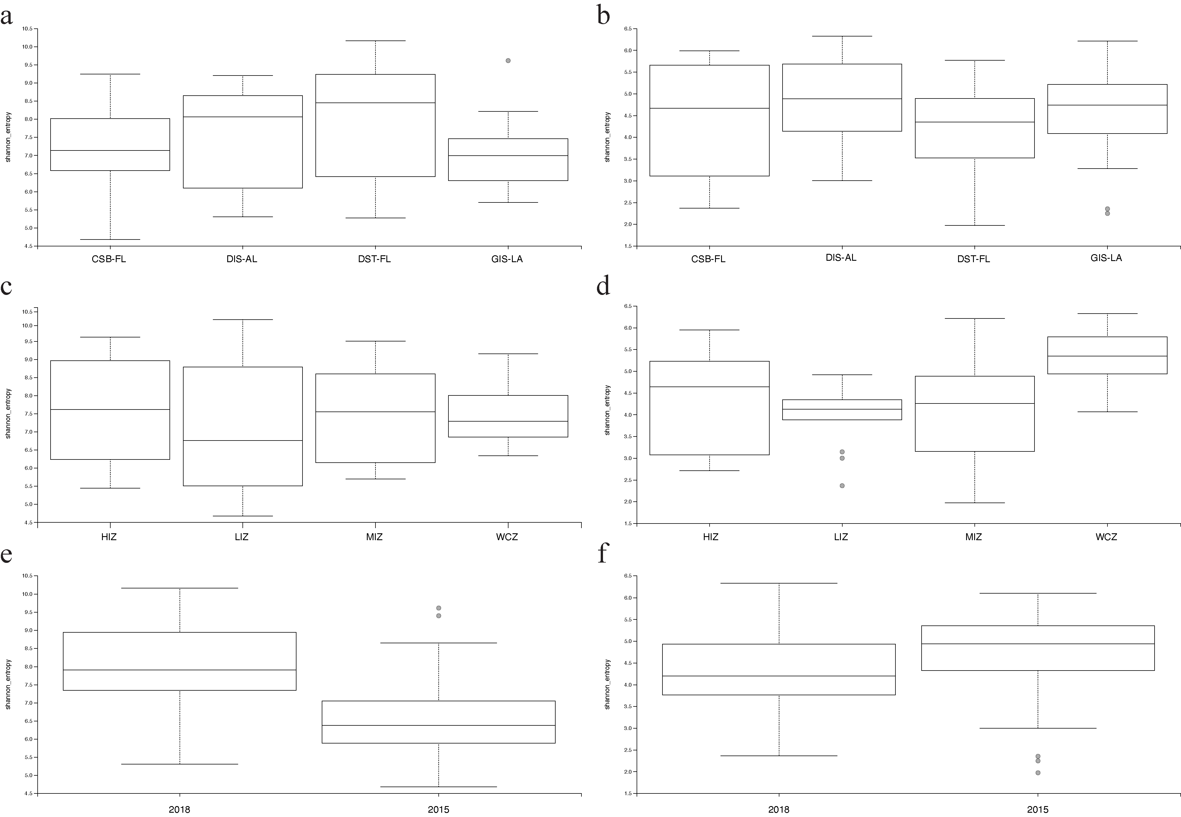
3.1. Alpha Diversity

Alpha diversity rarefaction curves showed that UPA samples required higher rarefaction depth than LSU samples for a reliable alpha diversity estimation (Figure S3). The rarefaction curves reached the major flattening at a depth of ~4500 reads and ~1300 reads for UPA and LSU markers, respectively, indicating that all samples had enough sequencing depth to be included in the diversity analyses.
All geographical locations showed relatively even average alpha diversity values based on Shannon and Faith’s PD indices (Figure 1a,b). There were no statistically significant alpha diversity differences in algae and entire communities with both molecular markers, p-value ≥ 0.05. However, there was a noticeable difference in alpha diversity between all samples collected in 2015 and 2018 from the same geographical location (e.g., GIS-2015 and GIS-2018). Alpha diversity was significantly higher (p-value ≤ 0.001) in 2018 for UPA-algae (Shannon index and Faith’s PD were significant) and UPA-all (only the Shannon index was significant). Therefore, samples were split into groups based on the sampling year, and the significance test was recalculated. After recalculation, samples from 2018 showed significantly different alpha diversity in algal communities based on geographic locations with both molecular markers and indices (UPA-algae: p-value ≤ 0.01, LSU-algae: p-value ≤ 0.05). However, there was no statistically significant difference in alpha diversity in the entire biotic community except for UPA-all based on the Shannon index (p-value = 0.0048). Additionally, the alpha diversity difference between the samples from 2015 remained statistically insignificant, p-value ≥ 0.05, which could be partially due to the lower number of sequenced samples from 2015.
Alpha diversity differences among zones were more statistically significant, with a median p-value ≤ 0.01 (only UPA’s Shannon p-value ≥ 0.05), than among geographical locations. LSU and UPA samples revealed significant alpha diversity among zones based on Faith’s PD index, but only LSU samples showed a significant difference based on the Shannon index (Table 1). Pairwise analysis indicated that the WCZ significantly differed from all other zones except for the HIZ. However, the alpha diversity difference between the WCZ and the HIZ was insignificant based only on Faith’s PD index of UPA-algae and UPA-all, which had nearly significant values (p-value = 0.0548 and p-value = 0.0736, respectively). However, there were almost no significant differences in alpha diversity among intertidal zones (HIZ, MIZ, and LIZ), except for between the HIZ and the LIZ and between the LIZ and the MIZ based on the Shannon index of LSU-all samples (p-value = 0.023 and 0.015, respectively). Overall, the WCZ had the highest average alpha diversity among all zones based on the LSU marker but one of the lowest based on the UPA marker (Figure 1).

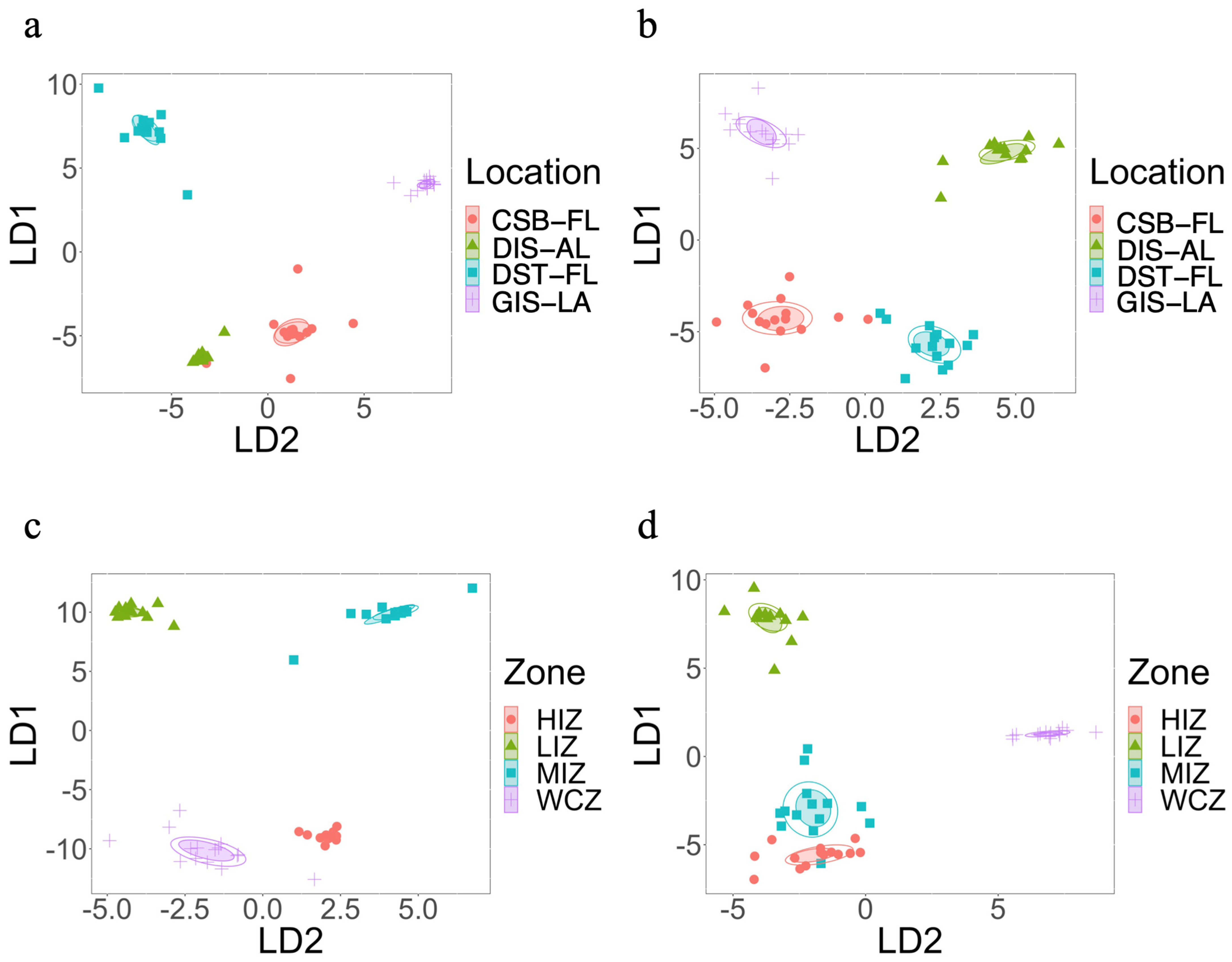
3.2. Beta Diversity Based on Geographical Locations

Geographical locations were a highly significant (p-value ≤ 0.0002) factor for differentiation between algal and entire biotic communities with both molecular markers and beta diversity distance calculation methods. Additionally, pairwise testing showed significant separation of each location from all others based on Bray–Curtis, with the highest p-value = 0.0287 and an average of 0.0038. The Weighted UniFrac metric did not show a significant difference between DST-FL samples and CSB-FL and DIS-AL samples. The only exception was the Weighted UniFrac distances of UPA-all, which had a p-value = 0.0094 between DST-FL and DIS-AL. However, after the separation of samples by the sampling year, only the DST-CSB pair maintained a p-value ≥ 0.05. A linear discriminant analysis (LDA) also placed algal communities from DST-FL and CSB-FL closest to each other in most cases (Figure 2b and Figure S4a,b). Overall, a higher similarity between CSB-FL and DST-FL biotic communities, which was revealed by eDNA in the current study, agrees with the actual geographic distances between these two sampled locations.

3.3. Beta Diversity Based on Zonation

All beta diversity methods applied in this study indicated that zonation had a statistically significant effect on beta diversity with a p-value ≤ 0.0001. Pairwise comparison between zones showed that, in total, five out of six zone pairs were significantly different from each other. The only zones that could not be significantly distinguished (p-value ≥ 0.1) were the MIZ and the LIZ, according to ANOSIM with any molecular marker or beta diversity metrics. Additionally, the beta diversity differences between zones had almost the same magnitude for the algae-only and entire biotic communities, with just a minor difference in p-values and R based on the ANOSIM pairwise test. Both molecular markers and beta diversity metrics showed that the WCZ was always significantly different from any intertidal zone. The HIZ and LIZ were consistently and significantly separated, but the significance between the HIZ and the MIZ depended on the choice of molecular marker and beta diversity calculation method. The comparison between the HIZ and the MIZ showed a significant difference with WU-UPA (p-value = 0.0433) but not with other methods, with an average p-value of 0.115. Additionally, LDA placed algal communities of the mid-intertidal zone closer to the low-intertidal area based on BC-UPA and BC-LSU dissimilarities (Figure S4c,d). However, the LDA of Weighted UniFrac distances depended more on the molecular marker (Figure 2c,d). WU-UPA placed HIZ and WCZ closer together, and WU-LSU placed HIZ and MIZ closer.

3.4. Beta Diversity Based on the Combination of Zone and Location

ANOSIM based on the combination of zones and geographical locations also indicated a highly significant (p-value ≤ 0.0001) association between a unique combination of sampled zones and locations (zone–location) and beta diversity for all samples (e.g., MIZ-CSB, WCZ-GIS, LIZ-DIS). However, evaluation based on the zone-location pairs significantly reduced the sample size for each group. In most cases, there were three samples per group (rarely four samples per group), which contained two samples collected in 2018 and one in 2015 (a few had two from 2018 and two from 2015). The LSU marker revealed the highest number of statistically significant pairwise analyses between zone–location pairs (Figure S3). BC-LSU showed 63 (out of 120), and WU-LSU showed 51 significantly separated zone-location communities. UPA showed fewer significantly different location-zone pairs, with 35 and 33 comparisons with a p-value ≤ 0.05 for Bray–Curtis dissimilarity and Weighted UniFrac distances, respectively. The increased variance can explain the relatively low ratio of significantly different zone–location pairs within groups due to the limited sample size for each unique zone–location combination.
Overall, the MIZ showed the best separation in the pairwise analysis of the same zones between the geographical locations (e.g., MIZ-GIS versus MIZ-CSB). MIZ-CSB versus MIZ-DIS and MIZ-CSB versus MIZ-GIS pairs significantly differed with markers and beta diversity estimation methods (p-value ≤ 0.03). The LIZ was the most similar zone between the geographical locations, with significantly different separations in three out of six comparisons. Additionally, a direct comparison of the same zones between the geographical areas indicated significant differences between all zones of CSB-FL and DIS-AL (e.g., HIZ-CSB versus HIZ-DIS, MIZ-CSB versus MIZ-CSB). The most similar locations were DIS-AL and DST-FL, which showed significant differences only between the HIZ and the WCZ. All other zones showed a significant difference in five out of six location pairs based on at least one molecular marker and beta diversity metric. LDA also did not indicate a straightforward grouping pattern. However, samples were generally grouped closer to each other according to the zone rather than the same geographical location, especially based on Weighted UniFrac distances (Figure S3).

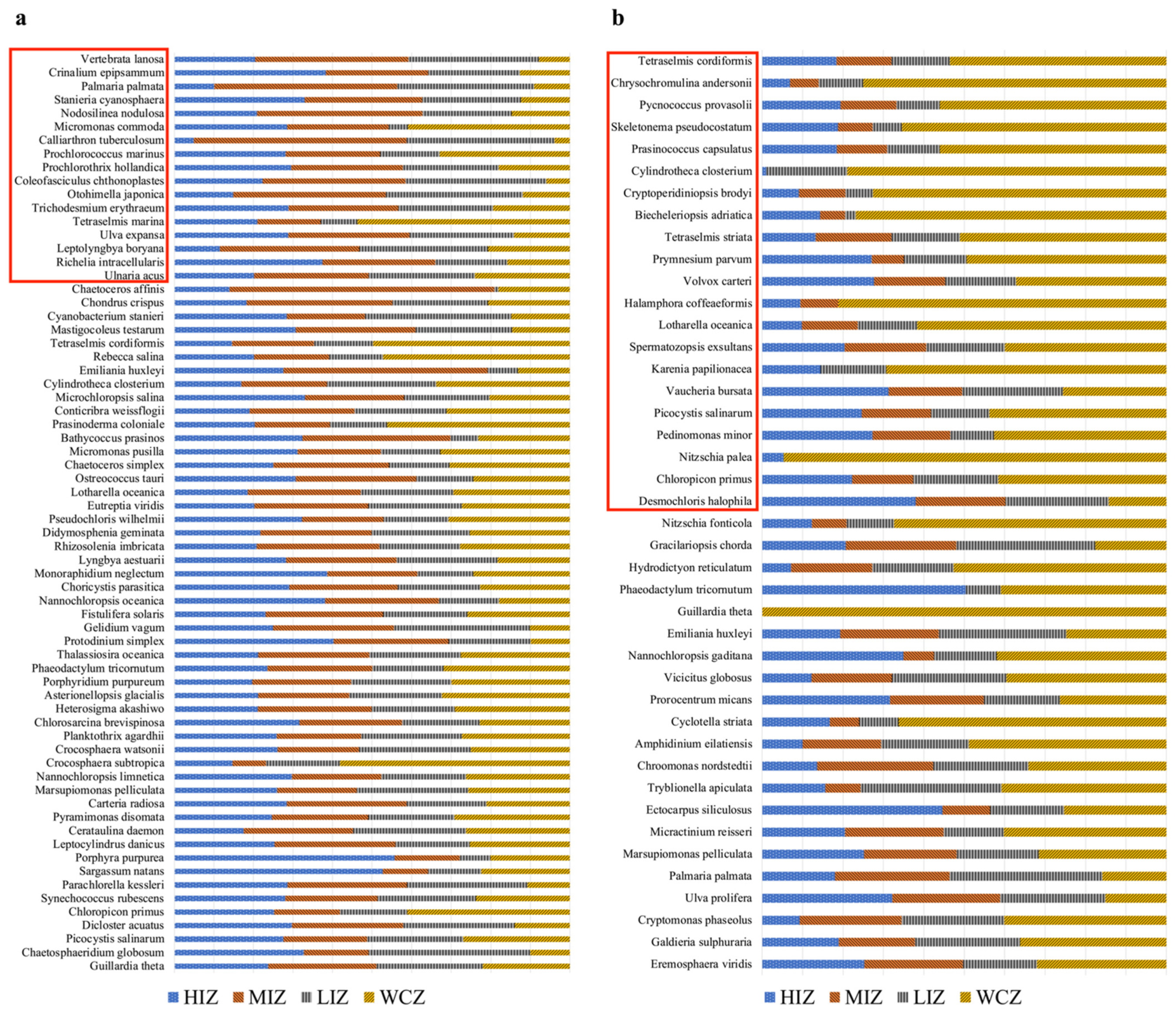
3.5. Algae Richness and Detected Non-Indigenous Species

This study recovered molecular signals of 179 species (including some strains, e.g., Synechococcus sp. CB0205) based on both markers, comprising 121 species of eukaryotic algae, 47 Cyanobacteria, and 11 non-algal protists species. Overall, 128 species were recovered by UPA and 50 species by LSU molecular markers. Identified eukaryotic algal species belonged to Bacillariophyta (twenty-four species), Chlorophyta (fifty-three species), Charophyta (one species), Cryptophyta (two species), Haptophyta (six species), Ochrophyta (thirteen species), Rhodophyta (twelve species), Dinophyceae (eight species), Euglenida (one species), and Chlorarachniophyceae (one species). Non-algal protists included species that belonged to Oomycota, Ciliophora, and photosynthetic amoeboids (Cercozoa). After removing strains that did not have the exact species name (for example, Synechococcus sp. CB0205), 96 algal species were recovered with UPA and 42 algal species with LSU (Table 2). Among the identified algal species, 12 species and 20 genera were recovered by both molecular markers. Therefore, overall, this study recovered molecular signals from 126 unique algal species and 136 unique algal genera. Likewise, 67 UPA and 42 LSU algal species had a total abundance ≥ 0.01% of the total number of amplicon reads (both taxonomically assigned and non-assigned).
Some of the collected algal samples were used for identification based on morphological characteristics for comparison with taxonomic assignments via eDNA analyses. Morphology-based identification confirmed 21 genera of micro- and macro-algae: Chaetoceros, Coscinodiscus, Cyclotella, Gelidium, Grateloupia, Leptocylindrus, Lyngbya, Pleurocapsa, Prorocentrum, Rhizosolenia, Sargassum, Skeletonema, Thalassiosira, Ulva, Cylindrotheca, Heterosigma, Leptocylindrus, Emiliania, Halamphora, Cryptomonas, and Tryblionella.
The algal species found in this study via eDNA included both native and non-indigenous species (Table 2 and Table S2), based on the available database records [38,62].
In total, 44 marine and brackish algal species identified in this study, of which 37 had and abundance ≥ 0.01% and were considered non-indigenous to the GoM region (Table S2), including Gelidium vagum, which is a documented alien species according to the World Register of Marine Species (WORMS) and AlgaeBase database records [38,62]. Furthermore, five of these non-indigenous species were detected by both molecular markers: Chloropicon primus, Palmaria palmata, Phaeodactylum tricornutum, Tetraselmis cordiformis, and Tetraselmis striata. The identified non-indigenous algal species showed higher relative abundance in the MIZ and WCZ according to the UPA and LSU markers, respectively (Figure 3). Furthermore, the current study recovered molecular signals of 28 freshwater algal species. Interestingly, four of these algal species were attributed to inhabiting the GoM according to WORMS and/or AlgaeBase despite being classified as a strictly freshwater species in the same databases. These freshwater species were Ulnaria acus, Cyclotella striata, Nitzschia fonticola, and Nitzschia palea. Overall, the identified freshwater algae included representatives such as Spermatozopsis exsultans, Cryptoperidiniopsis brodyi, and Nitzschia fonticola, which were three times more abundant in the WCZ than in any intertidal zone based on the LSU marker (Figure 3b). Unlike species identified by LSU, the freshwater algal species recovered by the UPA marker showed the highest average abundance in the HIZ and MIZ (Figure 3a). However, only four algal species had significantly different abundances between the zones: Leptolyngbya boryana, Prochlorothrix hollandica, Stanieria cyanosphaera, and Ulnaria acus (Figure 3a).

4. Discussion

4.1. Algal Community Differentiation

A slightly better separation in response to geographical location, based on Bray–Curtis dissimilarity over Weighted UniFrac distances, can be explained by the higher sensitivity of the weighted UniFrac metric to noise in the data [63]. Additionally, it seems reasonable that the Weighted UniFrac metric performed better in separating samples based on zones rather than geographic locations, as it places greater emphasis on deeper branches of the phylogeny [64]. Phylogenetically closer organisms are likely found in places with similar environmental stressors [65,66]. Considering that the average distance between the sampled geographical locations in this study was ~167.19 km (~103.91 miles), environmental stressors along the horizontal gradient should be more similar than along the vertical gradient [27], which is in agreement with the results of this investigation.

4.2. Detected Algal Species and Their Distribution

This study recovered molecular signals of 76 algal species (forty-seven marine, twenty-four freshwater, and five others), which were not documented in the GoM according to WORMS/AlgaeBase. However, 28 of these algal species have also been found in the GoM by previous eDNA studies according to the Global Biodiversity Information Facility (GBIF) records [67,68,69,70,71]. Therefore, this study recovered the molecular signal of 44 algal species, which were previously unreported for the GoM by any other source employed during this study. Additionally, nearly twice as many algal species were identified using the UPA compared to the LSU molecular marker. However, the majority of sequences recovered with the UPA marker belonged to Cyanobacteria. Therefore, LSU can be considered superior to UPA when the identification of eukaryotic algae, particularly those belonging to Miozoa, is prioritized. Additionally, the available molecular references for the UPA marker are dominated by Cyanobacteria species (395 out of 1228 records), while those for the LSU marker are predominantly Miozoa species (943 out of 1144 records), which undoubtedly contribute to the identification capabilities of each molecular marker.
The relative abundance of native and non-indigenous algal species recovered by eDNA in this study matched previously known habitat distribution patterns. Intertidal species such as Calliarthron tuberculosum and Ulva expansa significantly dominated the MIZ and LIZ (Figure 3a). Ulva prolifera and Porphyra umbilicalis showed the highest abundance in the HIZ, followed by the MIZ (Figure 3), which matches the natural distribution pattern of these species [72,73]. Algal species considered non-indigenous to the GoM also showed distributions between the zones in agreement with their native habitat patterns. For example, Palmaria palmata showed a significantly higher abundance in the MIZ and LIZ, correctly matching the known zonation for this species [74,75]. Although some known intertidal species (e.g., Gelidium vagum) did not show a statistically significant separation among the sampled zones, the relative abundance of such species was noticeably higher in the intertidal zones than in the water column (water sample) zone.
Environmental DNA signals from freshwater species detected in this study were probably brought by multiple rivers that discharge into the NGoM. Stoeckle et al. [76] showed that an eDNA signal of freshwater mollusks could be detected within ~3200 m (100–400 m optimal) downstream from the original population. Deiner and Altermatt (2014) also demonstrated that the eDNA signal of the two lake-dwelling species, Daphnia longispina and Unio tumidus, could be identified with a species resolution within ~10,000 m of the outflowing river (discharge ~3.6 m3/s) [77]. Overall, the biomass of the original population, distance, and flow speed are all essential factors for detecting eDNA signals downstream [78,79]. In addition, some of the algal species currently considered to inhabit freshwater environments are capable of persisting under higher salinity conditions. For example, Prochlorothrix hollandica, which has been detected in the current study but inhabits only freshwater environments according to AlgaeBase records, can grow with 170 mM NaCl (~34% seawater) when the supplied water comes from estuaries [80]. Additionally, the DNA signal of Prochlorothrix has been previously reported in the Baltic Sea [81]. Stanieria cyanosphaera, which is also considered to be a freshwater species according to AlgaeBase records, has been reported by Molina-Menor et al. (2019) as one of the most abundant species in the supralittoral zone of the Mediterranean Western coast. S. cyanosphaera was identified via high-throughput 16S rRNA and metagenomic sequencing [82]. Our results agreed with Molina-Menor, Tanner, Vidal-Verdu, Pereto and Porcar [82], who reported that S. cyanosphaera showed the highest abundance in the HIZ. Furthermore, the freshwater algal species identified in this study appeared up to three times higher in relative abundance in the WCZ than in any intertidal zone. This observation supports that detected freshwater species were delivered by freshwater inflow.
The current study reported an assessment of littoral algal communities across multiple littoral zones and locations along the coastline; therefore, to the best of our knowledge, this study represents the most detailed evaluation of littoral algal communities via eDNA metabarcoding. The results of our research indicated that coastal algal communities could be distinguished between the littoral zones and geographical locations through eDNA metabarcoding. In addition, we recovered the molecular signal of 121 eukaryotic algal species and 47 Cyanobacterial species (in total, 126 unique algal species), including native and non-indigenous algal species for the GoM region. Furthermore, here we provided an improved version of the algal reference database designed for eDNA metabarcoding studies of algal communities.

Supplementary Materials

The following supporting information can be downloaded at: https://www.mdpi.com/article/10.3390/phycology4040033/s1, Figure S1. The map of sampled geographical locations along the coastline of the Northern Gulf of Mexico. Figure S2. Schematic representation of the sampled intertidal zones: high intertidal zone (HIZ), middle intertidal zone (MIZ), and low intertidal zone (LIZ). The image was created at the time of the lowest tide level. Figure S3. Alpha diversity rarefaction curve based on the Shannon index. (a) UPA-GL, (b) LSU-GL, (c) UPA-ZN, (d) LSU-ZN. Figure S4. Linear discriminant analyses of algal communities based on Bray–Curtis dissimilarity among geographical locations (GL) and littoral zones (ZN). Table S1: The total number of sequenced samples from each zone and location. Table S2. All identified algal species. Algal species that were recovered by both markers are in bold. NIS stands for non-indigenous species.

Author Contributions

Conceptualization, S.B. and J.M.L.-B.; methodology, S.B. and J.M.L.-B.; formal analysis, S.B. and A.B.; data curation, S.B.; writing—original draft preparation, S.B.; writing—review and editing, S.B., J.M.L.-B., and B.W.; supervision, J.M.L.-B.; visualization, S.B. and A.B.; funding acquisition, S.B. and J.M.L.-B. All authors have read and agreed to the published version of the manuscript.

Funding

This work was supported in part by the Department of Biological Sciences and Graduate School of The University of Alabama to Sergei Bombin.

Institutional Review Board Statement

Not applicable.

Informed Consent Statement

Not applicable.

Data Availability Statement

Sequencing data and reference database generated in this study have been posted on 27 June 2024 and are publicly available via the Figshare online repository. https://doi.org/10.6084/m9.figshare.26120032.v1.

Acknowledgments

We thank Daryl W. Lam for his insightful comments on the manuscript.

Conflicts of Interest

The authors declare no conflicts of interest.

Abbreviations

ASVAmplicon sequence variant
CSBCape San Blas
DISDauphin Island
DSTDestin
eDNAenvironmental DNA
GISGrand Isle
HIZHigh-intertidal zone
LIZLow-intertidal zone
MIZMiddle-intertidal zone
NGoMNorthern Gulf of Mexico
WCZwater column zone

References

  1. Fautin, D.; Dalton, P.; Incze, L.S.; Leong, J.A.; Pautzke, C.; Rosenberg, A.; Sandifer, P.; Sedberry, G.; Tunnell, J.W., Jr.; Abbott, I.; et al. An overview of marine biodiversity in United States waters. PLoS ONE 2010, 5, e11914. [Google Scholar] [CrossRef]
  2. Kumpf, H.; Steidinger, K.; Sherman, K. The Gulf of Mexico Large Marine Ecosystem: Assessment, Sustainability, and Management; Blackwell Science: Malden, MA, USA, 1999. [Google Scholar]
  3. National Oceanic and Atmospheric Administration. The Gulf of Mexico at a Glance: A Second Glance; U.S. Department of Commerce: Washington, DC, USA, 2011. [Google Scholar]
  4. Tunnell, J.W.; Cato, J.C.; Felder, D.L.; Earle, S.A.; Camp, D.K.; Buster, N.A.; Holmes, C.W. Gulf of Mexico Origin, Waters, and Biota: Volume 2, Ocean and Coastal Economy; Texas A&M University Press: College Station, TX, USA, 2009; Volume 2. [Google Scholar]
  5. Ward, C.H. Habitats and Biota of the Gulf of Mexico: Before the Deepwater Horizon Oil Spill: Volume 2: Fish Resources, Fisheries, Sea Turtles, Avian Resources, Marine Mammals, Diseases and Mortalities; Springer: Berlin/Heidelberg, Germany, 2017; Volume 2. [Google Scholar]
  6. Fredericq, S.; Cho, T.O.; Earle, S.A.; Gurgel, C.F.; Krayesky, D.M.; Mateo-Cid, L.E.; Mendoza-González, A.C.; Norris, J.N.; Suárez, A.M. Seaweeds of the Gulf of Mexico. In Gulf of Mexico Origin, Waters and Biota; Texas A&M University Press: College Station, TX, USA, 2009; Volume 1, pp. 187–259. [Google Scholar]
  7. Davidson, A.D.; Campbell, M.L.; Hewitt, C.L.; Schaffelke, B. Assessing the impacts of non-indigenous marine macroalgae: An update of current knowledge. Bot. Mar. 2015, 58, 55–79. [Google Scholar] [CrossRef]
  8. Bartolo, A.G.; Zammit, G.; Peters, A.F.; Küpper, F.C. The current state of DNA barcoding of macroalgae in the Mediterranean Sea: Presently lacking but urgently required. Bot. Mar. 2020, 63, 253–272. [Google Scholar] [CrossRef]
  9. Baker, P.; Baker, S.; Fajans, J. Nonindigenous Marine Species in the Greater Tampa Bay Ecosystem. Tampa Bay Estuary Program Technical Publication, 2004, 02–04. Available online: https://pinellas.wateratlas.usf.edu/upload/documents/NonindigenousMarineSpeciesGreatTampaBayEcosystem.pdf (accessed on 15 February 2021).
  10. Ji, Y.; Ashton, L.; Pedley, S.M.; Edwards, D.P.; Tang, Y.; Nakamura, A.; Kitching, R.; Dolman, P.M.; Woodcock, P.; Edwards, F.A.; et al. Reliable, verifiable and efficient monitoring of biodiversity via metabarcoding. Ecol. Lett. 2013, 16, 1245–1257. [Google Scholar] [CrossRef] [PubMed]
  11. Pawlowski, J.; Esling, P.; Lejzerowicz, F.; Cedhagen, T.; Wilding, T.A. Environmental monitoring through protist next-generation sequencing metabarcoding: Assessing the impact of fish farming on benthic foraminifera communities. Mol. Ecol. Resour. 2014, 14, 1129–1140. [Google Scholar] [CrossRef] [PubMed]
  12. Pawlowski, J.; Lejzerowicz, F.; Apotheloz-Perret-Gentil, L.; Visco, J.; Esling, P. Protist metabarcoding and environmental biomonitoring: Time for change. Eur. J. Protistol. 2016, 55, 12–25. [Google Scholar] [CrossRef] [PubMed]
  13. Pochon, X.; Wood, S.A.; Keeley, N.B.; Lejzerowicz, F.; Esling, P.; Drew, J.; Pawlowski, J. Accurate assessment of the impact of salmon farming on benthic sediment enrichment using foraminiferal metabarcoding. Mar. Pollut. Bull. 2015, 100, 370–382. [Google Scholar] [CrossRef] [PubMed]
  14. Ardura, A.; Borrell, Y.J.; Fernández, S.; González Arenales, M.; Martínez, J.L.; Garcia-Vazquez, E. Nuisance Algae in Ballast Water Facing International Conventions. Insights from DNA Metabarcoding in Ships Arriving in Bay of Biscay. Water 2020, 12, 2168. [Google Scholar] [CrossRef]
  15. Visco, J.A.; Apotheloz-Perret-Gentil, L.; Cordonier, A.; Esling, P.; Pillet, L.; Pawlowski, J. Environmental Monitoring: Inferring the Diatom Index from Next-Generation Sequencing Data. Environ. Sci. Technol. 2015, 49, 7597–7605. [Google Scholar] [CrossRef] [PubMed]
  16. Apotheloz-Perret-Gentil, L.; Cordonier, A.; Straub, F.; Iseli, J.; Esling, P.; Pawlowski, J. Taxonomy-free molecular diatom index for high-throughput eDNA biomonitoring. Mol. Ecol. Resour. 2017, 17, 1231–1242. [Google Scholar] [CrossRef] [PubMed]
  17. Lejzerowicz, F.; Esling, P.; Pillet, L.; Wilding, T.A.; Black, K.D.; Pawlowski, J. High-throughput sequencing and morphology perform equally well for benthic monitoring of marine ecosystems. Sci. Rep. 2015, 5, 13932. [Google Scholar] [CrossRef] [PubMed]
  18. Aylagas, E.; Rodriguez-Ezpeleta, N. Analysis of Illumina MiSeq Metabarcoding Data: Application to Benthic Indices for Environmental Monitoring. Methods Mol. Biol. 2016, 1452, 237–249. [Google Scholar] [CrossRef]
  19. Bell, K.L.; Burgess, K.S.; Okamoto, K.C.; Aranda, R.; Brosi, B.J. Review and future prospects for DNA barcoding methods in forensic palynology. Forensic Sci. Int. Genet. 2016, 21, 110–116. [Google Scholar] [CrossRef]
  20. Cowart, D.A.; Pinheiro, M.; Mouchel, O.; Maguer, M.; Grall, J.; Mine, J.; Arnaud-Haond, S. Metabarcoding is powerful yet still blind: A comparative analysis of morphological and molecular surveys of seagrass communities. PLoS ONE 2015, 10, e0117562. [Google Scholar] [CrossRef] [PubMed]
  21. Sherwood, A.R.; Dittbern, M.N.; Johnston, E.T.; Conklin, K.Y. A metabarcoding comparison of windward and leeward airborne algal diversity across the Ko ‘olau mountain range on the island of O’ahu, Hawaii. J. Phycol. 2017, 53, 437–445. [Google Scholar] [CrossRef] [PubMed]
  22. Djemiel, C.; Plassard, D.; Terrat, S.; Crouzet, O.; Sauze, J.; Mondy, S.; Nowak, V.; Wingate, L.; Ogée, J.; Maron, P.-A. µgreen-db: A reference database for the 23S rRNA gene of eukaryotic plastids and cyanobacteria. Sci. Rep. 2020, 10, 5915. [Google Scholar] [CrossRef] [PubMed]
  23. Lebret, K.; Tesson, S.V.; Kritzberg, E.S.; Tomas, C.; Rengefors, K. Phylogeography of the freshwater raphidophyte Gonyostomum semen confirms a recent expansion in northern Europe by a single haplotype. J. Phycol. 2015, 51, 768–781. [Google Scholar] [CrossRef] [PubMed]
  24. Wolf, D.I.; Vis, M.L. Stream algal biofilm community diversity along an acid mine drainage recovery gradient using multimarker metabarcoding. J. Phycol. 2020, 56, 11–22. [Google Scholar] [CrossRef] [PubMed]
  25. Chappuis, E.; Terradas, M.; Cefalì, M.E.; Mariani, S.; Ballesteros, E. Vertical zonation is the main distribution pattern of littoral assemblages on rocky shores at a regional scale. Estuar. Coast. Shelf Sci. 2014, 147, 113–122. [Google Scholar] [CrossRef]
  26. Burkett, V.; Fernandez, L.; Nicholls, R.; Woodroffe, C. Climate change impacts on coastal biodiversity. In Climate Change and Biodiversity in the Americas; Fenech, A., MacIver, D., Dallmeier, F., Eds.; Environment Canada: Ottawa, ON, Canada, 2008; pp. 167–193. [Google Scholar]
  27. Valdivia, N.; Scrosati, R.A.; Molis, M.; Knox, A.S. Variation in community structure across vertical intertidal stress gradients: How does it compare with horizontal variation at different scales? PLoS ONE 2011, 6, e24062. [Google Scholar] [CrossRef]
  28. Veiga, P.; Rubal, M.; Vieira, R.; Arenas, F.; Sousa-Pinto, I. Spatial variability in intertidal macroalgal assemblages on the North Portuguese coast: Consistence between species and functional group approaches. Helgol. Mar. Res. 2013, 67, 191. [Google Scholar] [CrossRef]
  29. Kokabi, M.; Yousefzadi, M.; Razaghi, M.; Feghhi, M.A. Zonation patterns, composition and diversity of macroalgal communities in the eastern coasts of Qeshm Island, Persian Gulf, Iran. Mar. Biodivers. Rec. 2016, 9, 96. [Google Scholar] [CrossRef]
  30. Sherwood, A.R.; Presting, G.G. Universal primers amplify a 23S rDNA plastid marker in eukaryotic algae and cyanobacteria 1. J. Phycol. 2007, 43, 605–608. [Google Scholar] [CrossRef]
  31. Leliaert, F.; De Clerck, O.; Verbruggen, H.; Boedeker, C.; Coppejans, E. Molecular phylogeny of the Siphonocladales (Chlorophyta: Cladophorophyceae). Mol. Phylogenet. Evol. 2007, 44, 1237–1256. [Google Scholar] [CrossRef] [PubMed]
  32. Bombin, S.; Wysor, B.; Lopez-Bautista, J.M. Assessment of littoral algal diversity from the northern Gulf of Mexico using environmental DNA metabarcoding. J. Phycol. 2021, 57, 269–278. [Google Scholar] [CrossRef]
  33. Bolger, A.M.; Lohse, M.; Usadel, B. Trimmomatic: A flexible trimmer for Illumina sequence data. Bioinformatics 2014, 30, 2114–2120. [Google Scholar] [CrossRef]
  34. Edgar, R.C. Search and clustering orders of magnitude faster than BLAST. Bioinformatics 2010, 26, 2460–2461. [Google Scholar] [CrossRef] [PubMed]
  35. Edgar, R.C.; Flyvbjerg, H. Error filtering, pair assembly and error correction for next-generation sequencing reads. Bioinformatics 2015, 31, 3476–3482. [Google Scholar] [CrossRef] [PubMed]
  36. Edgar, R.C. UNOISE2: Improved error-correction for Illumina 16S and ITS amplicon sequencing. bioRxiv 2016. bioRxiv:081257. [Google Scholar]
  37. Callahan, B.J.; McMurdie, P.J.; Holmes, S.P. Exact sequence variants should replace operational taxonomic units in marker-gene data analysis. ISME J. 2017, 11, 2639. [Google Scholar] [CrossRef] [PubMed]
  38. Guiry, M.; Guiry, G. AlgaeBase. Available online: https://www.algaebase.org (accessed on 11 September 2021).
  39. Holovachov, O.; Haenel, Q.; Bourlat, S.J.; Jondelius, U. Taxonomy assignment approach determines the efficiency of identification of OTUs in marine nematodes. R. Soc. Open Sci. 2017, 4, 170315. [Google Scholar] [CrossRef] [PubMed]
  40. Katoh, K.; Standley, D.M. MAFFT multiple sequence alignment software version 7: Improvements in performance and usability. Mol. Biol. Evol. 2013, 30, 772–780. [Google Scholar] [CrossRef] [PubMed]
  41. Nguyen, L.T.; Schmidt, H.A.; von Haeseler, A.; Minh, B.Q. IQ-TREE: A fast and effective stochastic algorithm for estimating maximum-likelihood phylogenies. Mol. Biol. Evol. 2015, 32, 268–274. [Google Scholar] [CrossRef]
  42. Kalyaanamoorthy, S.; Minh, B.Q.; Wong, T.K.F.; von Haeseler, A.; Jermiin, L.S. ModelFinder: Fast model selection for accurate phylogenetic estimates. Nat. Methods 2017, 14, 587–589. [Google Scholar] [CrossRef] [PubMed]
  43. Hoang, D.T.; Chernomor, O.; von Haeseler, A.; Minh, B.Q.; Vinh, L.S. UFBoot2: Improving the Ultrafast Bootstrap Approximation. Mol. Biol. Evol. 2018, 35, 518–522. [Google Scholar] [CrossRef]
  44. Bolyen, E.; Rideout, J.R.; Dillon, M.R.; Bokulich, N.A.; Abnet, C.C.; Al-Ghalith, G.A.; Alexander, H.; Alm, E.J.; Arumugam, M.; Asnicar, F. Reproducible, interactive, scalable and extensible microbiome data science using QIIME 2. Nat. Biotechnol. 2019, 37, 852–857. [Google Scholar] [CrossRef]
  45. Barbera, P.; Kozlov, A.M.; Czech, L.; Morel, B.; Darriba, D.; Flouri, T.; Stamatakis, A. EPA-ng: Massively Parallel Evolutionary Placement of Genetic Sequences. Syst. Biol. 2019, 68, 365–369. [Google Scholar] [CrossRef] [PubMed]
  46. Czech, L.; Barbera, P.; Stamatakis, A. Genesis and Gappa: Processing, analyzing and visualizing phylogenetic (placement) data. Bioinformatics 2020, 36, 3263–3265. [Google Scholar] [CrossRef] [PubMed]
  47. Tomas, C.R. Identifying Marine Phytoplankton; Elsevier: Amsterdam, The Netherlands, 1997. [Google Scholar]
  48. Dhargalkar, V.; Kavlekar, D. Seaweeds—A Field Manual. 2004. Available online: https://drs.nio.res.in/drs/bitstream/handle/2264/96/Seaweeds-Manual.pdf?sequence=1&isAllowed=y (accessed on 18 September 2019).
  49. Woelkerling, W.J. Marine Plants of the Caribbean. A Field Guide from Florida to Brazil. Phycologia 1989, 28, 537. [Google Scholar] [CrossRef]
  50. Whittaker, R.H. Evolution and measurement of species diversity. Taxon 1972, 21, 213–251. [Google Scholar] [CrossRef]
  51. Lozupone, C.A.; Hamady, M.; Kelley, S.T.; Knight, R. Quantitative and qualitative β diversity measures lead to different insights into factors that structure microbial communities. Appl. Environ. Microbiol. 2007, 73, 1576–1585. [Google Scholar] [CrossRef]
  52. Chang, Q.; Luan, Y.; Sun, F. Variance adjusted weighted UniFrac: A powerful beta diversity measure for comparing communities based on phylogeny. BMC Bioinform. 2011, 12, 118. [Google Scholar] [CrossRef]
  53. Straub, D.; Blackwell, N.; Langarica-Fuentes, A.; Peltzer, A.; Nahnsen, S.; Kleindienst, S. Interpretations of Environmental Microbial Community Studies Are Biased by the Selected 16S rRNA (Gene) Amplicon Sequencing Pipeline. Front. Microbiol. 2020, 11, 550420. [Google Scholar] [CrossRef] [PubMed]
  54. Reitmeier, S.; Hitch, T.C.; Fikas, N.; Hausmann, B.; Ramer-Tait, A.E.; Neuhaus, K.; Berry, D.; Haller, D.; Lagkouvardos, I.; Clavel, T. Handling of spurious sequences affects the outcome of high-throughput 16S rRNA gene amplicon profiling. ISME Commun. 2021, 1, 31. [Google Scholar] [CrossRef]
  55. Weiss, S.; Xu, Z.Z.; Peddada, S.; Amir, A.; Bittinger, K.; Gonzalez, A.; Lozupone, C.; Zaneveld, J.R.; Vázquez-Baeza, Y.; Birmingham, A. Normalization and microbial differential abundance strategies depend upon data characteristics. Microbiome 2017, 5, 27. [Google Scholar] [CrossRef] [PubMed]
  56. Bokulich, N.A.; Subramanian, S.; Faith, J.J.; Gevers, D.; Gordon, J.I.; Knight, R.; Mills, D.A.; Caporaso, J.G. Quality-filtering vastly improves diversity estimates from Illumina amplicon sequencing. Nat. Methods 2013, 10, 57–59. [Google Scholar] [CrossRef]
  57. Venables, W.; Ripley, B. Random and mixed effects. In Modern Applied Statistics with S; Springer: Berlin/Heidelberg, Germany, 2002; pp. 271–300. [Google Scholar]
  58. Wickham, H. ggplot2. Wiley Interdiscip. Rev. Comput. Stat. 2011, 3, 180–185. [Google Scholar] [CrossRef]
  59. Paulson, J.N.; Stine, O.C.; Bravo, H.C.; Pop, M. Differential abundance analysis for microbial marker-gene surveys. Nat. Methods 2013, 10, 1200–1202. [Google Scholar] [CrossRef]
  60. Paulson, J.N.; Pop, M.; Bravo, H.C. metagenomeSeq: Statistical analysis for sparse high-throughput sequencing. Bioconductor Package 2013, 1, 191. [Google Scholar]
  61. Caporaso, J.G.; Kuczynski, J.; Stombaugh, J.; Bittinger, K.; Bushman, F.D.; Costello, E.K.; Fierer, N.; Pena, A.G.; Goodrich, J.K.; Gordon, J.I.; et al. QIIME allows analysis of high-throughput community sequencing data. Nat. Methods 2010, 7, 335–336. [Google Scholar] [CrossRef] [PubMed]
  62. Horton, T.; Kroh, A.; Ahyong, S.; Bailly, N.; Boyko, C.B.; Brandão, S.N.; Gofas, S.; Hooper, J.N.A.; Hernandez, F.; Holovachov, O.; et al. World Register of Marine Species (WoRMS). 2020. Available online: https://www.marinespecies.org/ (accessed on 11 September 2021).
  63. Fukuyama, J.; McMurdie, P.J.; Dethlefsen, L.; Relman, D.A.; Holmes, S. Comparisons of distance methods for combining covariates and abundances in microbiome studies. In Biocomputing 2012; World Scientific: Singapore, 2012; pp. 213–224. [Google Scholar]
  64. Fukuyama, J. Emphasis on the deep or shallow parts of the tree provides a new characterization of phylogenetic distances. Genome Biol. 2019, 20, 131. [Google Scholar] [CrossRef] [PubMed]
  65. Burns, J.H.; Strauss, S.Y. More closely related species are more ecologically similar in an experimental test. Proc. Natl. Acad. Sci. USA 2011, 108, 5302–5307. [Google Scholar] [CrossRef]
  66. Godoy, B.S.; Camargos, L.M.; Lodi, S. When phylogeny and ecology meet: Modeling the occurrence of Trichoptera with environmental and phylogenetic data. Ecol. Evol. 2018, 8, 5313–5322. [Google Scholar] [CrossRef] [PubMed]
  67. MGnify. ADDOMEx Tier 3 Experiments: Mesocosm Si with Gulf of Mexico Coastal Waters. 2018. Available online: https://www.gbif.org/dataset/552346e7-47c0-425c-9fbd-cb0366759db1 (accessed on 10 May 2021).
  68. MGnify. Amplicon Sequencing of Tara Oceans DNA Samples Corresponding to Size Fractions for Protists. 2018. Available online: https://www.gbif.org/dataset/d596fccb-2319-42eb-b13b-986c932780ad (accessed on 10 May 2021).
  69. MGnify. Marine Water Column Samples Targeted Loci Environmental. 2019. Available online: https://www.gbif.org/dataset/51fd12e4-402a-4271-94f8-9d5727af1cda (accessed on 11 May 2021).
  70. MGnify. Temporal Effect of Plant Diversity and Oiling on Nitrogen Cycling in Marsh Sediments. 2019. Available online: https://www.gbif.org/dataset/93c02d72-d8ac-4396-8522-bd7c8dbbd62d (accessed on 11 May 2021).
  71. MGnify. Effects of Triclosan on Bacterial Community Composition in Natural Seawater Microcosms. 2019. Available online: https://www.gbif.org/dataset/2d312e17-bd09-45ec-834c-9a372a0c7e8e (accessed on 11 May 2021).
  72. Titlyanov, E.A.; Titlyanova, T.V.; Li, X.; Huang, H. Common Marine Algae of Hainan Island (Guidebook). In Coral Reef Marine Plants of Hainan Island; Titlyanov, E.A., Titlyanova, T.V., Li, X., Huang, H., Eds.; Academic Press: Cambridge, MA, USA, 2017; pp. 75–228. [Google Scholar]
  73. Green, L.A.; Neefus, C.D. The effects of short-and long-term freezing on Porphyra umbilicalis Kützing (Bangiales, Rhodophyta) blade viability. J. Exp. Mar. Biol. Ecol. 2014, 461, 499–503. [Google Scholar] [CrossRef]
  74. Saunders, G.W.; Jackson, C.; Salomaki, E.D. Phylogenetic analyses of transcriptome data resolve familial assignments for genera of the red-algal Acrochaetiales-Palmariales Complex (Nemaliophycidae). Mol. Phylogenet Evol. 2018, 119, 151–159. [Google Scholar] [CrossRef]
  75. Rødde, R.S.H.; Vårum, K.M.; Larsen, B.A.; Myklestad, S.M. Seasonal and geographical variation in the chemical composition of the red alga Palmaria palmata (L.) Kuntze. Bot. Mar. 2004, 47, 125–133. [Google Scholar] [CrossRef]
  76. Stoeckle, B.C.; Beggel, S.; Kuehn, R.; Geist, J. Influence of stream characteristics and population size on downstream transport of freshwater mollusk environmental DNA. Freshw. Sci. 2021, 40, 191–201. [Google Scholar] [CrossRef]
  77. Deiner, K.; Altermatt, F. Transport distance of invertebrate environmental DNA in a natural river. PLoS ONE 2014, 9, e88786. [Google Scholar] [CrossRef]
  78. Jane, S.F.; Wilcox, T.M.; McKelvey, K.S.; Young, M.K.; Schwartz, M.K.; Lowe, W.H.; Letcher, B.H.; Whiteley, A.R. Distance, flow and PCR inhibition: E DNA dynamics in two headwater streams. Mol. Ecol. Resour. 2015, 15, 216–227. [Google Scholar] [CrossRef] [PubMed]
  79. Wacker, S.; Fossøy, F.; Larsen, B.M.; Brandsegg, H.; Sivertsgård, R.; Karlsson, S. Downstream transport and seasonal variation in freshwater pearl mussel (Margaritifera margaritifera) eDNA concentration. Environ. DNA 2019, 1, 64–73. [Google Scholar] [CrossRef]
  80. Pinevich, A.; Velichko, N.; Ivanikova, N. Cyanobacteria of the genus prochlorothrix. Front. Microbiol. 2012, 3, 173. [Google Scholar] [CrossRef] [PubMed]
  81. Geiss, U.; Bergmann, I.; Blank, M.; Schumann, R.; Hagemann, M.; Schoor, A. Detection of Prochlorothrix in brackish waters by specific amplification of pcb genes. Appl. Environ. Microbiol. 2003, 69, 6243–6249. [Google Scholar] [CrossRef]
  82. Molina-Menor, E.; Tanner, K.; Vidal-Verdu, A.; Pereto, J.; Porcar, M. Microbial communities of the Mediterranean rocky shore: Ecology and biotechnological potential of the sea-land transition. Microb. Biotechnol. 2019, 12, 1359–1370. [Google Scholar] [CrossRef] [PubMed]
Figure 1. Alpha diversity distributions of identified algal communities. Diversity is calculated using the Shannon index. Samples are grouped based on the geographical location: (a) UPA-algae and (b) LSU-algae, zones: (c) UPA-algae and (d) LSU-algae, and sampling year: (e) UPA-algae and (f) LSU-algae. The boxplots display the distribution of alpha diversity values: the horizontal line within each box represents the median, the edges of the box show the interquartile range (IQR), and the whiskers indicate variability outside the IQR up to 1.5 times the IQR. Outliers are represented by individual points beyond the whiskers.
Phycology 04 00033 g001
Figure 2. Linear discriminant analyses of algal communities based on Weighted UniFrac distances among geographical locations (GL) and littoral zones (ZN). (a) UPA-GL, (b) LSU-GL, (c) UPA-ZN, and (d) LSU-ZN.
Phycology 04 00033 g002
Figure 3. Algal species distribution among zones. Only algal species with an abundance ≥ 0.01% were included. (a) shows species recovered by the UPA and (b) LSU molecular markers. Species arranged in order from smallest to largest p-values obtained via the Kruskal–Wallis test. Framed species have a p-value ≤ 0.05.
Phycology 04 00033 g003
Table 1. Statistical significance of differences in alpha and beta diversity. Significance is based on geographical locations (GL), zones (ZN), and sampling year (SY). Asterisks indicate the significance of comparisons: *** for p-value ≤ 0.001, ** for p-value ≤ 0.01, and * for p-value ≤ 0.05.
SamplesShannonFaith’s PD BCWU
UPA-algaeGL, ZN, SY ***GL, ZN *, SY ***GL ***, ZN ***GL ***, ZN ***
UPA-allGL, ZN, SY ***GL, ZN **, SYGL ***, ZN ***, GL ***, ZN ***
LSU-algaeGL, ZN **, SYGL, ZN **, SYGL ***, ZN ***GL ***, ZN ***
LSU-allGL, ZN **, SYGL, ZN **, SYGL ***, ZN ***GL ***, ZN ***
Table 2. Summary of all identified algal species. NIS stands for non-indigenous species. Twelve alga species were shared by UPA and LSU markers: Chloropicon primus, Cylindrotheca closterium, Ectocarpus siliculosus, Emiliania huxleyi, Guillardia theta, Lotharella oceanica, Marsupiomonas pelliculata, Palmaria palmata, Phaeodactylum tricornutum, Picocystis salinarum, Tetraselmis cordiformis, and Tetraselmis striata.
MarkersAlgal Species TotalNative GoMMarine/Brackish NISInconclusive
Status
Freshwater
Species
UPA9615331724
LSU42111694
Disclaimer/Publisher’s Note: The statements, opinions and data contained in all publications are solely those of the individual author(s) and contributor(s) and not of MDPI and/or the editor(s). MDPI and/or the editor(s) disclaim responsibility for any injury to people or property resulting from any ideas, methods, instructions or products referred to in the content.

