Simple Summary
Dairy cows excrete nitrogen in their urine, which can cause environmental problems. Calculating the daily amount of urine excreted is essential to evaluating the nitrogen emissions of individual farms. Methods were developed to calculate the amount of urine reliably using creatinine in urine as an indicator. The statistical analysis showed that calculation methods can be used for modern dairy and dry cows. It was also revealed that it is possible to calculate the amount of urine without knowing the cow’s body weight, allowing calculations to be made under farm conditions.
Abstract
A key factor in calculating dairy cows’ nitrogen (N) excretion is knowing the amount of daily excreted urine. The present study aimed to investigate two methods to calculate the daily urine volume (UV) excreted using spot urine samples. Data were obtained from nine balance experiments involving 47 lactating and seven non-lactating German Holstein cows, with an average body weight (BW) of 620 ± 95 kg and an average age of 5.6 ± 1.4 years. Daily urinary creatinine (Cr) and UVs were known for all animals. The first method was developed by linearly regressing the daily excreted amount of Cr in urine against BW (p < 0.001; R2 = 0.51; RSE: 2.8). The slope of the regression was used to calculate UV. The second method includes a non-linear regression of UV on Cr concentration in urine, allowing direct estimation of UV without knowledge of BW (p < 0.001; RSE: 8.13). Both estimation methods were compared to the standard method to determine UV from balance trials using Lin’s concordance correlation coefficient (CCC) and Bland–Altman plots. The first method had a CCC of 0.81, and the second method had a CCC of 0.85. Both methods can confidently be applied to calculate UV. Therefore, the second method is usable if BW is unavailable.
1. Introduction
It is generally acknowledged in animal nutrition that the nitrogen excretions of dairy cows are an important source of nitrogen emissions in livestock farming [1,2]. Germany has set a binding target to reduce nitrogen emissions by 2030 as part of its national and EU environmental commitments [3]. To achieve this goal, improvement in livestock balance in dairy farms is necessary [4].
In dairy cows, 66–72% of total N intake is excreted through feces and urine [5,6,7,8]. The kidneys excrete most of the N as urea (U). U in urine is then transformed to ammonia by enzymatic processes in the environment. Reducing U in urine is key to minimizing ammonia emissions [9]. U in urine can be easily reduced through feeding. The amount of excreted urinary U results from urine volume (UV) and N-concentration in urine, which can be influenced by dilution effects [10]. Therefore, the calculation of total urinary N excretion of dairy cows relies on the knowledge of the amount of urine excreted.
Although the primary aim of this study is methodological, this environmental context explains the significance of accurately estimating urine volume more generally. Under practical farm conditions, direct measurement of total urine volume is not possible. Therefore, robust and reliable estimation methods are needed to support the monitoring and control of nitrogen fluxes in dairy farming. This includes the need to evaluate existing methods and validate them under current conditions—especially for modern dairy cow genetics and for physiologically different groups such as both lactating and dry cows.
Previous studies [11,12,13,14] examined the effects of various nutritional factors on urinary N excretion using a balance technique enabling total urine collection. However, such a technique can only be applied under experimental conditions using a few animals. In practical feeding setups, urine samples can be used to evaluate N-reducing feeding strategies. A calculation of urine volume is required to determine total nitrogen excretion.
Although methods for UV estimation based on creatinine (Cr) concentration have been published [15,16], their direct applicability to modern Holstein cows may need re-evaluation. Although some educational books refer to the problem with dry cows, to our knowledge there is a shortage of published data on the applicability of existing UV calculation methods in this animal group.
It is not to meant to question the general validity of creatinine-based methods, but to recognize that breeding over the years has affected the relationship between BW, muscle mass and creatinine excretion [17,18]. The same holds for dry cows as their body composition changes markedly, particularly in the last weeks of gravidity [19]. In addition, BW is rarely known in dairy farms, which further complicates the practical use of current methods.
One aim of the present study was to re-evaluate published methods for estimating UV based on Cr concentration and BW and to test a calculation method that does not rely on the knowledge of BW. While the data are from a defined research setting, the approach aims to provide insights that may be relevant beyond the immediate study context.
Moreover, for such estimation methods, it is also essential to know whether urinary spot samples are representative of the whole UV in terms of Cr concentration. Therefore, the second aim of the present examinations was to evaluate the relationships between Cr concentrations in spot samples and total UV obtained from the same cows.
2. Materials and Methods
2.1. Experimental Design and Animals
Urine amounts of 47 lactating and 7 non-lactating German Holstein dairy cows collected in nine balance experiments were used to investigate (1) the relationships between Cr concentration in spot and pooled urine samples (Experiment 9) and (2) the associations between urinary Cr concentration and excretion, and UV (Experiments 1 to 9) (Table 1). All experiments occurred at the Friedrich-Loeffler-Institut, Institute of Animal Nutrition in Braunschweig, Germany. Each experiment lasted 26 days, beginning with a 21-day adaptation period for adaptation to the experimental diet, followed by a 5-day balance period where urine and feces were collected quantitatively. Each experiment used 5 to 7 cows. All cows were housed in a temperature-controlled barn and tethered with a rope around their necks.

Table 1.
Mean and standard deviation of variables of experiments 1–9.
Lactating cows were three to eight years old. They were in their first to fifth lactation and 143 ± 52 days in milk. Dry cows were five to eight years old and had already completed four to six lactations. BW of all cows was determined at the start of each experiment and was 620 ± 95 kg on average.
Lactating cows were milked at 5:30 AM and 3:30 PM daily. They had ad libitum access to fresh water in individual drinking bowls at all times. The composition of the diets varied according to the experimental questions. Therefore, rations contained varying proportions of maize silage and concentrate feed (Table 1).
2.2. Sample Collection
As mentioned above, quantitative urine collection lasted five days in all experiments. It was achieved using urine devices attached to the cow’s pubic area via contact adhesive. The urine devices consisted of a leather funnel connected to a pressure-resistant polyvinylchloride tube, which led to a covered canister positioned behind the cow. The leather adhered around the cow’s genital area to form an airtight and waterproof seal against the skin, enclosing the vulva. This setup ensured the separation of feces and urine and enabled the accurate and clean collection of the entire UV. Urine was weighed and homogenized daily.
In experiment 9, spot urine samples were collected from cows in the morning. Therefore, 50 mL of urine was collected externally when a cow urinated spontaneously. If no spontaneous urination occurred, the remaining urine from the last excretion in the polyvinyl chloride tube was used.
2.3. Analyses
Both daily pooled and spot urine samples underwent analysis for Cr concentration. The urine samples were homogenized at room temperature by shaking. Dilution with purified water was performed at a ratio of 1:50, and then the sample was filtered and analyzed using an HPLC system (Shimadzu, Kyoto, Japan). The following two solvents were used for good separation conditions, especially for Cr. Solvent A contained 0.5% acetonitrile (MeCN), 10 mmol/l o-phosphoric acid, and 10 mmol/l 1-hexanesulfonic acid sodium salt monohydrate in a water-based solution. For Solvent B, MeCN was used [20]. Cr concentration was determined via duplicate measurements.
2.4. Calculation and Statistics
2.4.1. Calculation
The daily excretion of Cr by each cow was calculated using the formula:
Daily Cr excretion in g = UV in L × Cr concentration in g/L,
The excretion of Cr per kg BW (BW) was calculated using the formula:
Cr excretion in g/d per kg BW = Cr excretion in g/d/BW in kg,
2.4.2. Statistics
Statistical analyses were performed using RStudio with R (version 4.3.0), while graphical presentations were created using the ggplot2 package.
The relationships between variables were analyzed using linear and non-linear regression analyses. Procedure lm() of base R was used for linear regressions, while procedure nlm() of base R was used for non-linear regression.
For evaluating agreement between different methods for the same target variable, concordance correlation coefficients (CCC) were estimated using the procedure ccc() of package DescTools version 0.99.48 [21], and Bland–Altman plots of package BlandAltmanLeh [22] were used.
To answer the first question, the mean Cr concentrations of spot samples were linearly regressed on the corresponding concentrations in the pooled sample.
Different linear and non-linear regressions, including prediction intervals, were calculated using base R to determine the calculation method.
Cr concentration in urine spot samples was compared with that in urine pool samples. For this, the mean Cr concentrations of spot samples were linearly regressed on the corresponding concentrations in the pooled sample. Mean concentrations of pooled samples were considered as the reference method. Lin’s concordance correlation coefficient (CCC), s.shift and l.shift were used to evaluate the accuracy and precision of the spot sample method.
Validation of whether Cr excretion is independent of the amount of urine excreted daily was performed by linear regression with daily UV in L as the dependent variable and the Cr excretion in g/day as the independent variable. The same was performed by linear regression with BW in kg as the dependent variable and Cr excretion in g/day as the independent variable. A significant difference in the slope of the regression lines between lactating and dry cows was tested using ANOVA. A t-test was used to determine the significance of BW differences between lactating and dry cows.
A regression was used to evaluate the independence between Cr concentration and UV, with Cr concentration (g/L) as the independent variable and UV (L) as the dependent variable.
Since residual analyses indicated no linear relationship, non-linear functions were fitted to the data using the Akaike Information Criterion (AIC) [23], Bayesian Information Criterion (BIC) [24] and Leave-One-Out Cross-Validation (LOOCV) [25] as quality criteria.
A power regression was performed with Cr concentration as the independent variable and UV as the dependent variable.
Linear regressions with UV (L/g) calculated by the linear or non-linear method as the dependent variable and collected UV (L/d) as the independent variable were performed. CCC, s.shift and l.shift were determined to evaluate the agreement and possible systematic deviations in position and scatter.
The package BlandAltmanLeh (version 0.3.1) created Bland–Altman plots to visualize method differences and evaluate systematic errors.
Bland–Altman plots compared the Cr concentrations in pooled and spot urine samples. Additionally, the urine volume estimated by a linear method was compared to the actual urine volume excreted.
The linear method was defined as follows:
Linear method = BW in kg × (29.5/Cr concentration in mg/L),
Another Bland–Altman plot was used to compare the amount of urine calculated using the power regression estimation equation with the actual amount of urine.
The non-linear method was defined as follows:
Non-linear method = 16.5 × (Cr concentration in g/L urineˆ−0.76),
3. Results
All statistical data below is based on the values shown in Table 1.
3.1. Comparison of Cr Concentrations Between Urine Pool and Urine Spot Samples
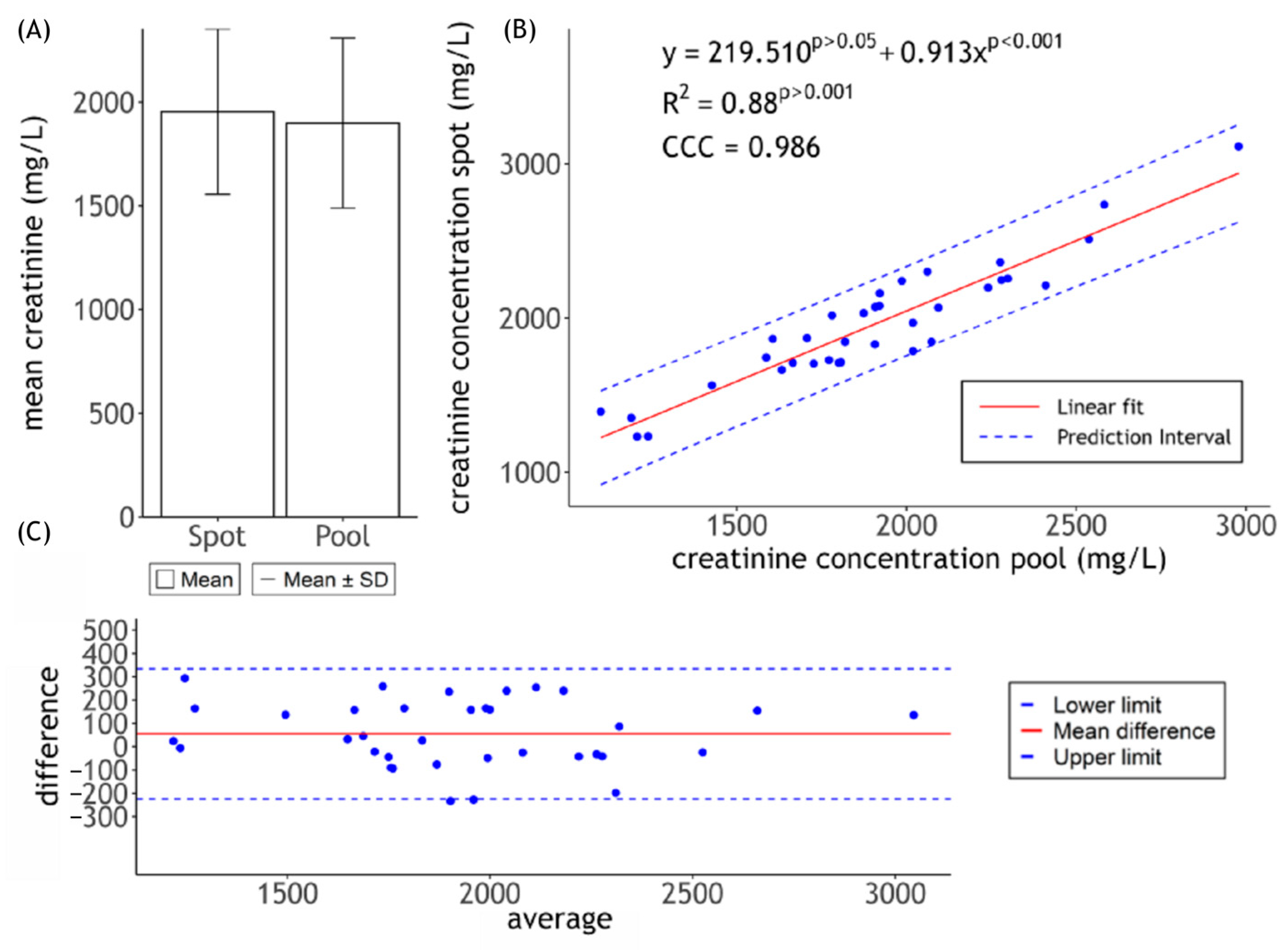
The intercept of the linear regression is 220 and is not significantly different from zero (p > 0.05), while the slope is 0.91 and highly significant (p < 0.001). The regression explains 88% of the total variance of the data. CCC is 0.99. All data points are evenly and closely distributed around the regression line and within the 95% prediction interval (see Figure 1B).

Figure 1.
Analysis of Cr concentrations in pooled and spot urine samples of dry cows. Data is derived from daily pool and spot samples of seven dry cows over the five following days (experiment 9). (A) Mean Cr concentration in spot and pool samples, error bars indicate standard deviation (SD). (B) Linear regression between Cr concentrations in spot and pool samples. The red solid line indicates the linear fit. Blue dashed lines show the upper and lower 95% prediction interval. CCC is the Concordance Correlation Coefficient. (C) Bland–Altman plot: the x-axis displays mean values between corresponding Cr concentrations in spot and pool samples, and the y-axis displays the related differences. The red solid line shows the average difference between the two methods. Blue dashed lines mark the 95% limits of agreement.
The average difference between the two methods is 55 mg Cr/L urine. Single data points scatter evenly along the full range of urine concentrations between methods and are within the 95% agreement limit (see Figure 1C).
3.2. Cr Amount in Relation to UV and BW
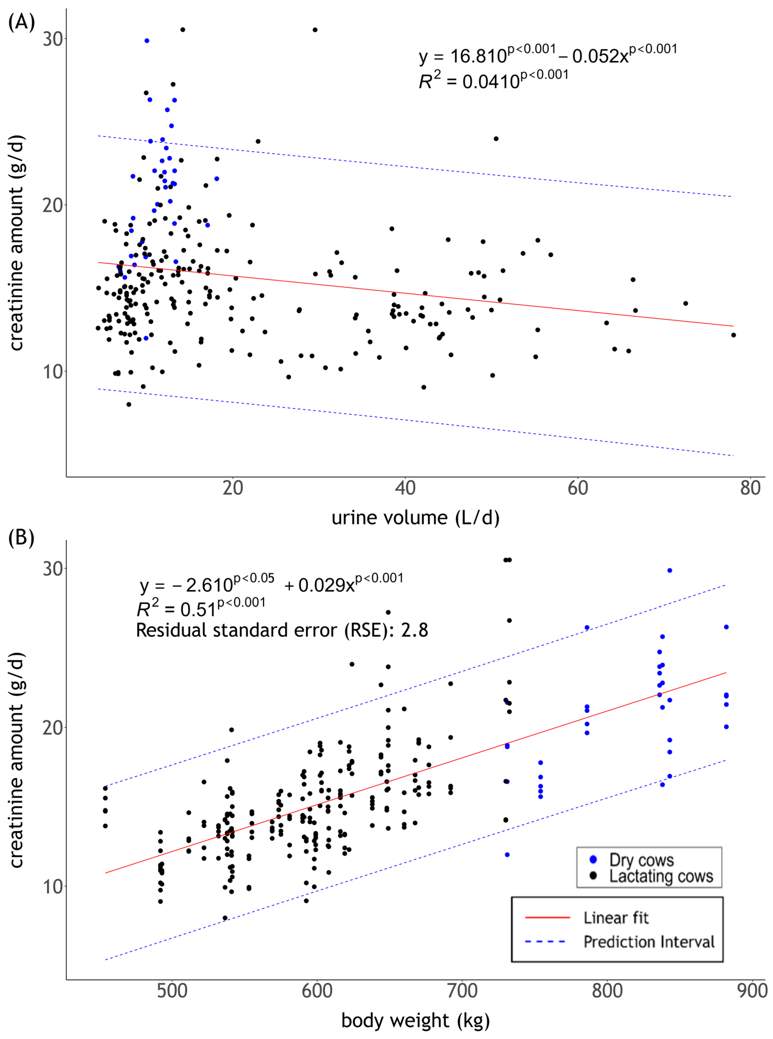
The intercept of the linear regression between Cr amount (g/d) as the independent variable and UV (L/d) as the dependent variable is 16.81 and significantly different from zero (p < 0.001), while the slope is −0.052 and highly significant (p < 0.001). The regression explains 4% of the total variance in the data.
The data points are widely distributed in the range of 10 and 30 g/d Cr, with the majority between 10 and 20 g/d. Data points at low UVs (up to 20 L/d) are widely scattered, with Cr levels ranging from below 10 to over 30 g/d. As UV increases, the amount of Cr tends to decrease, and the points are located between 10 and 20 g/d along the descending regression line. A few outliers, especially at UVs above 60 L/d, are further away. Some points exceed the 95% prediction interval, while most are evenly and closely distributed around the regression line.
The t-test between BW of lactating cows and dry cows shows highly significant differences (p < 0.001).
The intercept of the linear regression is −2.6 and is significantly different from zero (p < 0.05), while the slope is 0.03 and highly significant (p < 0.001). The regression explains 51% of the total variance in the data.
Data points are evenly and closely distributed around the regression line. Most points are within the 95% prediction interval, while some data points rise above the 95% prediction interval, and a few falls below. Linear regression indicates that the amount of Cr excreted daily increases by 29.5 g for every 1 kg increase in BW. The residual standard error is 2.8 g of Cr excreted (see Figure 2B).
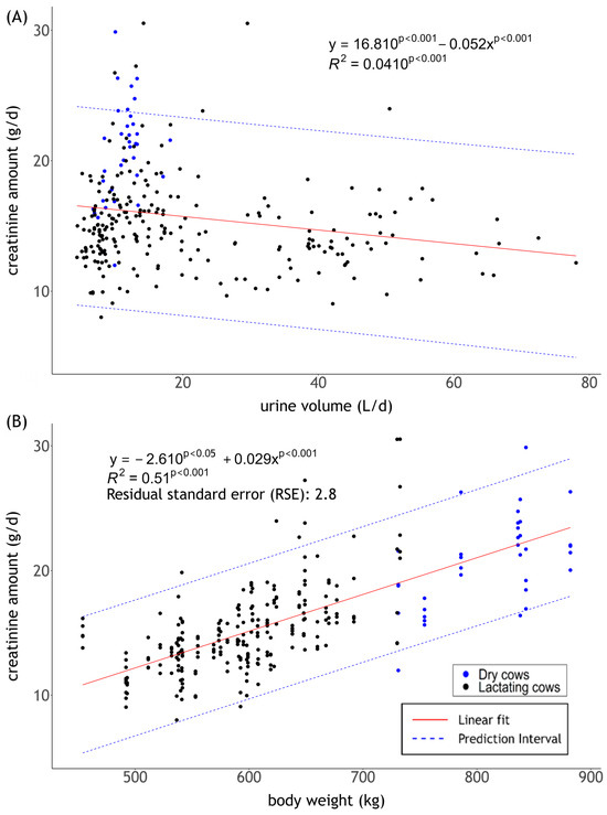
Figure 2.
Cr amounts excreted with urine in dependence on (A) UV and (B) BW of dry and lactating cows. Data is generated from urine samples of 7 dry and 48 lactating cows over the five consecutive days (experiment 1–9). Dry cows are represented by data points colored in blue, and data points in black represent lactating cows. Red solid lines display the linear regression. Blue dashed lines indicate the upper and lower 95% prediction intervals.
3.3. UV in Correlation to Cr Concentration
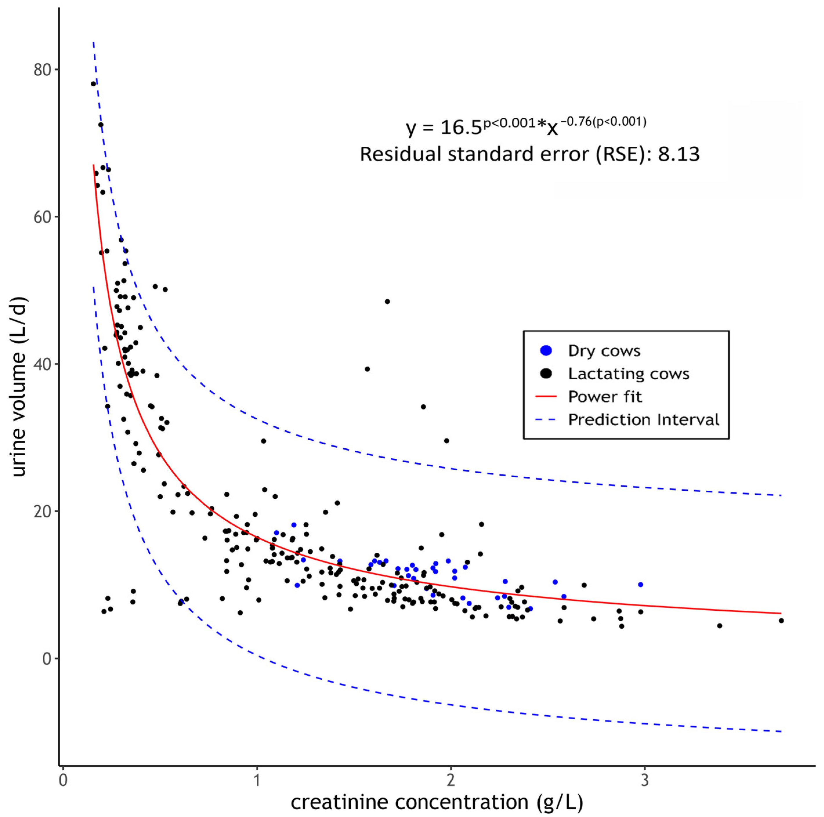
The intercept of power regression is 16.5 and significantly different from zero (p < 0.001), while the slope is −0.76 and highly significant (p < 0.001). The residual standard error is 8.13 L UV excreted per day.
Some outliers are visible at low Cr concentrations, mainly above or a few below the prediction interval, but most are within this interval. The data points scatter closely to the regression line. The highest variation in UV is shown at low Cr concentrations, which leads to an increase in the power regression curve at less than 1 g Cr.
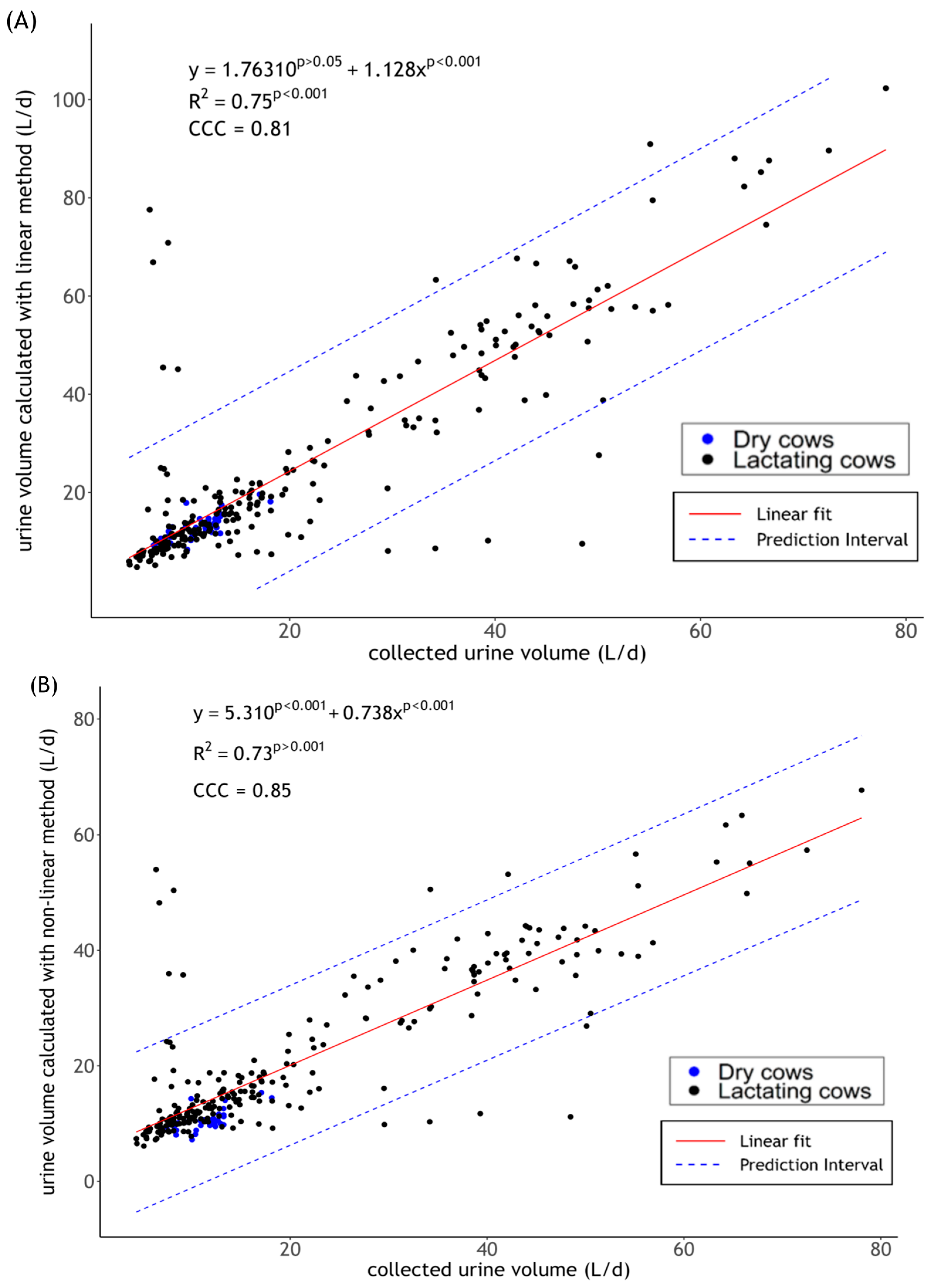
The intercept of linear regression is 1.76 and not significantly different from zero (p > 0.05), while the slope is 1.13 and highly significant (p < 0.001). The regression explains 75% of the total variance in the data. CCC is 0.81. L.shift is calculated at −0.24 and s.shift at 0.77.
Some outliers are visible at higher UV above 40 L/d, mainly above the prediction interval, and a few below, but most are within this interval. The data points scatter closely to the regression line (see Figure 3).
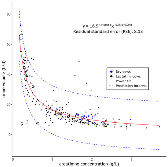
Figure 3.
Relation between UV and Cr concentration. Depicted are data of urine samples from 7 dry and 48 lactating cows over the five consecutive days (experiment 1–9). Dry cows are represented by data points colored in blue, and data points in black represent lactating cows. A power regression with Cr concentration as the independent variable and UV as the dependent variable. The red solid curve indicates the regression. Blue dashed curves display the upper and lower 95% prediction intervals.
The intercept of linear regression is 5.31 and significantly different from zero (p < 0.001), while the slope is 0.74 and highly significant (p < 0.001). The regression explains 73% of the total variance in the data. CCC is 0.85. L.shift is calculated at −0.01 and s.shift at 1.16.
Some outliers are visible at higher UV above 40 L/d, mainly above or a few below the prediction interval, but most are within this interval. Data points scatter less than in Figure 4A, and the prediction interval is closer. The data points scatter closely to the regression line. (see Figure 4B).
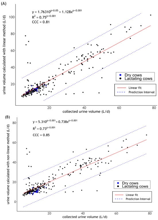
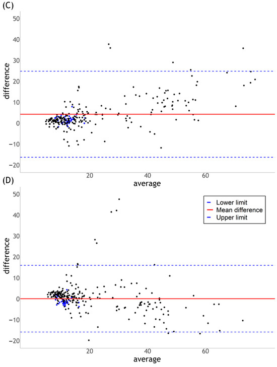
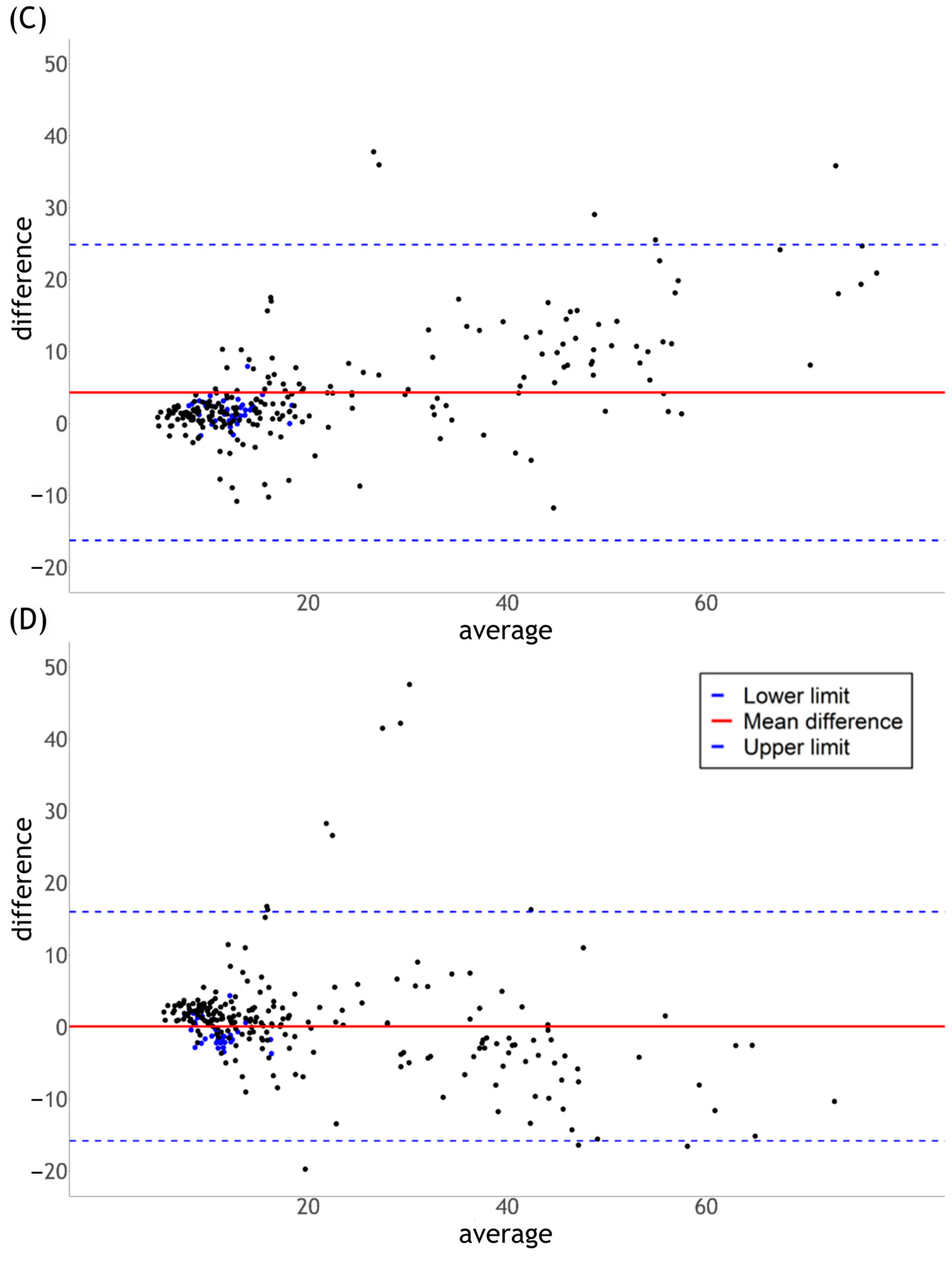
Figure 4.
Internal validation of UV estimation using the linear (A,C) and the non-linear method (B,D) to actual UV. Data is derived from urine samples of 7 dry and 48 lactating cows over the five consecutive days (experiment 1–9). Dry cows are represented by data points colored in blue, and data points in black represent lactating cows. (A,B) Linear regression between collected UV and calculated UV. The red solid line indicates the linRStudioear fit. Blue dashed lines show the upper and lower 95% prediction interval. (C,D) Bland–Altman plot: the x-axis displays mean values of calculated and collected UV, and the y-axis displays the related differences in the distribution. The red solid line shows the average difference between the two methods. Blue dashed lines mark the 95% limits of agreement.
The average difference between the linear method and measured UV is 4.3. The lower limit is −16.2, and the upper limit is 24.9. An upward drift in differences is shown when the average UV exceeds 40 L. Despite this, differences are evenly distributed over the range of the average values, with few outliers and narrow limits of agreement. (see Figure 4C).
The average difference between the non-linear method and measured UV is 0.1. Limits of agreement range from −15.8 to 16. Differences display a downward drift when the average UV increases above 40 L. Some outliers exceed the upper limit between an average UV of 20 L to 30 L. Beyond that, the differences are within the limits and evenly distributed across the average value range (Figure 4D).
4. Discussion
Estimating UV under practical farm conditions relies on the representativeness of the Cr concentrations measured in spot samples for total UV. Therefore, we validated the relationships between the Cr concentrations measured in spot samples and the total urine collected from the same cows.
Spot samples are particularly relevant in practice due to their simplicity and practicality. This study shows that measuring Cr concentration in spot samples reliably estimates daily Cr excretion, with no baseline difference between methods (see Figure 1).
Collecting with the urinals connected to the containers and using the Cr concentrations in these urine pool samples is considered the gold standard method. This constancy is caused by the origin of muscle metabolism, which works at a stable rate under constant physiological conditions. Cr is defined as a continuous excretion parameter throughout the day. The Cr production does not fluctuate throughout the day. Using spot samples instead does not require the laborious and time-consuming collection of pool samples and does not limit the number of usable animals. It is particularly suitable for continuous practice monitoring of urinary parameters. Studies have already been carried out where the Cr concentration in spot samples was analyzed. Cr concentration with the dependence on the UV changes throughout the day [26,27]. This biological mechanism ensures that daily Cr excretion indicates muscle mass and remains largely unaffected by short-term nutritional or environmental factors. Another study [28] shows a higher agreement of the estimated UV when the Cr concentration is calculated from six spot samples distributed over the day. There is an agreement in the Cr concentration of spot samples taken in the morning compared to the Cr concentration of pool samples for one of the feeding groups. Data quality could be improved by taking several spot samples throughout the day and comparing the Cr concentrations between them.
Cr is a metabolic product that is synthesized from creatine phosphate in endogenous muscle metabolism when ATP required for muscle work is produced by phosphate splitting. In this way, Cr is formed in a constant daily amount. The daily excreted Cr depends on the body’s muscle mass [26,29]. It makes Cr one of the few substances excreted in the urine that does not undergo metabolism and is freely filtered by the kidneys without secretion or reabsorption, regardless of water intake [30,31]. Due to its constant production and the fact that it is not reabsorbed in the kidneys, it is an excellent marker for estimating UV [31]. Therefore, the BW of the dairy cow and the mean daily excretion of Cr have been used to establish the estimation equations for UV calculation in the past [15,16].
However, breeding developments have altered the body composition of modern Holstein cattle. Studies suggest that the proportion of muscle mass to BW may have decreased as breeding has increasingly focused on milk production [17,18]. These considerations clarify that UV estimation models based on Cr must be evaluated against changing physiological starting conditions due to genetic breeding and different production stages. The body composition of dry cows is also subject to considerable fluctuations, particularly in the last few weeks before calving, as fat and muscle reserves develop differently [19]. These physiological changes could affect the accuracy of UV calculation methods.
The collected Cr amount relative to BW in the current data showed results consistent with other studies and within the physiological range [15,16,29,31].
An interesting observation is that dry cows had a higher Cr excretion than lactating cows (see Figure 2B). This fact correlates with higher muscle mass and higher Cr excretion. The BW of the cow is a significant factor affecting the amount of Cr excreted daily. As Cr is a degradation product of muscle metabolism, Cr excretion increases with increasing muscle mass and BW. Multiple studies show that larger, heavier animals excrete more Cr per day [26,29]. It remains to be questioned whether the average amount of Cr excreted per kilogram of BW also applies to cows with a different muscle-to-fat ratio, as beef breeds.
The literature reports that the average Cr concentration in cow urine ranges from 0.25 to 0.8 g/L [32]. In the current experiments, daily measured Cr concentrations are above the physiological average described there, while the minimum concentration is below. Older studies report higher average Cr concentrations, around 1.5 g/L [27], which better match our observed values.
The scientific literature provides evidence that the acid in the solvent used for Cr analysis does not influence the Cr concentration as a reliable marker for total urine excretion [33]. A different acid was used in this publication.
However, varying Cr concentrations could depend on higher or lower UV. Dairy cows excrete a daily average of 15 to 30 L of urine [15,16]. The collected UV data show urine amounts within the normal physiological range. The observed variance in urine excretion could be explained by factors such as differences in water intake or the foreign body sensitivity caused by urinals. Despite thoroughly examining outliers, no clear patterns or causes could be identified based on the available information. Furthermore, the method of collecting urine with urinals, which is considered the gold standard, is nevertheless not entirely error-free.
Figure 3 shows that the Cr concentration in urine cannot increase if UV is 20 L or more. It may suggest that the maximum glomerular filtration rate has been reached. When urine volume (UV) is high, the Cr concentration levels off, which might mean the kidneys cannot filter or concentrate more Cr. When UV is low, the body reabsorbs water in the kidneys, increasing the concentration of Cr in the urine. The inverse link between Cr and UV makes sense because more urine means more dilution. It is physiologically plausible, as increased water intake increases diuresis and dilutes urine substances such as Cr. Still, using a power model to describe this adds complexity. Especially at low Cr levels, the model might reflect kidney limits, which should be studied more closely. Understanding these physiological boundaries is essential for improving model precision, especially at the extremes of the UV distribution.
The previously mentioned fluctuation in Cr concentration throughout the day should be considered. The amount of Cr filtered in the kidney depends on the individual, hydration status, physical activity, and the time of sampling regarding food intake. The kidney function, such as the glomerular filtration rate, also plays a role [31,32]. These factors demonstrate the dynamic nature of renal physiology and its influence on the stability of biomarkers in spot urine samples.
Even with differences between individual animals, the results from Experiment 9 are statistically strong and reliable. Tracking individual factors in future studies could help explain their influence more clearly.
The linear model tends to overestimate urine output, as the uneven agreement limits show. This pattern suggests that the model could be improved, especially at higher urine volumes. The deviations are particularly pronounced at higher UVs, suggesting the equation does not scale well in this range. Despite a positive mean bias, which increases the tendency to overestimate, the linear regression indicates a proportional relationship and generally good predictability (see Figure 4A,C). In addition, the linear method has a lower residual standard deviation, which indicates a lower calculation deviation (Figure 2 and Figure 4). However, this raises the question of whether a correction of the estimation equation is necessary for larger UVs.
The non-linear method, in contrast, shows an almost neutral bias, indicating a much better agreement with the actual UVs excreted. Tighter limits of agreement indicate an overall higher consistency and accuracy than the Cr-based estimation method. However, the slope and intercept deviate more strongly from the optimal value, which makes interpretation more difficult. While the concordance correlation coefficient (CCC) indicates a slightly higher agreement, the coefficient of determination (R2) remains lower than that of the linear method (see Figure 4B,D). This fact indicates that despite the better agreement of the values with the non-linear method, the predictive power is not superior in all aspects. Therefore, a method-specific approach may be necessary, depending on the application. Ultimately, the choice of estimation method may depend on physiological variability and specific research or practical application goals, especially when working on marginal UV.
5. Conclusions
The results confirm that both methods—one relying on body weight and one not—can provide appropriate estimates of urine volume in both lactating and dry cows. Spot urine samples proved to be a practical approach that reflected adequate creatinine concentrations compared to total urine volume collected under controlled conditions. While the results confirm the usability of established methods, they also point to the need for careful interpretation, especially when daily variations in creatinine excretion are not considered.
Spot urine sampling therefore represents a feasible alternative to urine volume estimation in cows and supports practicability in the field without affecting accuracy.
Future work could focus on quantifying the amount of daily variation in creatinine excretion and developing correction factors to improve the accuracy of urine volume estimates under different physiological and environmental conditions.
Author Contributions
Conceptualization, K.P., U.M., D.v.S. and S.D.; methodology, K.P., S.D. and F.B.; software, K.P. and F.B.; validation, K.P., S.D. and C.V.; formal analysis, K.P., S.D. and F.B.; investigation, D.v.S.; data curation, K.P.; writing—original draft preparation, K.P.; writing—review and editing, K.P., U.M., D.v.S., S.D., F.B., C.U., L.H. and C.V.; visualization, K.P.; supervision, U.M., S.D. and C.V.; project administration, U.M.; funding acquisition, U.M. All authors have read and agreed to the published version of the manuscript.
Funding
This work is financially supported by the Federal Ministry of Food and Agriculture (BMEL) based on a decision of the Parliament of the Federal Republic of Germany, granted by the Federal Office for Agriculture and Food (BLE; grant number 28N204802).
Institutional Review Board Statement
The animal study protocol was approved by Lower Saxony State Office for Consumer Protection and Food Safety (LAVES, Oldenburg, Germany).
Informed Consent Statement
Not applicable.
Data Availability Statement
Inquiries can be directed to the corresponding author and are available at https://doi.org/10.5281/zenodo.15432147.
Acknowledgments
The authors thank the co-workers of the Institute of Animal Nutrition and the co-workers of the experimental station of the Friedrich-Loeffler-Institute in Brunswick for their great support, as well as other members of the MoMiNe team.
Conflicts of Interest
The authors declare no conflicts of interest.
Abbreviations
The following abbreviations are used in this manuscript:
| AIC | Akaike Information Criterion |
| BIC | Bayesian Information Criterion |
| BW | Body Weight |
| CCC | Concordance Correlation Coefficient |
| Cr | Creatinine |
| LOOCV | Leave-One-Out Cross-Validation |
| N | Nitrogen |
| RSE | Residual Standard Error |
| SD | Standard deviation |
| U | Urea |
References
- Korevaar, H. The nitrogen balance on intensive Dutch dairy farms—A review. Livest. Prod. Sci. 1992, 31, 17–27. [Google Scholar] [CrossRef]
- Sorley, M.; Casey, I.; Styles, D.; Merino, P.; Trindade, H.; Mulholland, M.; Zafra, C.R.; Keatinge, R.; Le Gallj, A.; O’Brien, D.; et al. Factors influencing the carbon footprint of milk production on dairy farms with different feeding strategies in western Europe. J. Clean. Prod. 2024, 435, 140104. [Google Scholar] [CrossRef]
- Bundesregierung. Deutsche Nachhaltigkeitsstrategie: Weiterentwicklung 2021; Bundesregierung, Presse-und Informationsamt der Bundesregierung, Ed.; Bundesregierung: Berlin, Germany, 2021.
- Umweltbundesamt. Ammoniakemissionen in der Landwirtschaft Mindern. Gute Fachliche Praxis; Kuratorium für Technik und Bauwesen in der Landwirtschaft e.V.: Dessau-Roßlau, Germany, 2021; p. 2021. [Google Scholar]
- Tamminga, S. Nutrition management of dairy cows as a contribution to pollution control. J. Dairy Sci. 1992, 75, 345–357. [Google Scholar] [CrossRef]
- Castillo, A.R.; Kebreab, E.; Beever, D.E.; France, J. A review of efficiency of nitrogen utilisation in lactating dairy cows and its relationship with environmental pollution. J. Anim. Feed Sci. 2000, 9, 1–32. [Google Scholar] [CrossRef]
- Spanghero, M.; Kowalski, Z.M. Updating analysis of nitrogen balance experiments in dairy cows. J. Dairy Sci. 2021, 104, 7725–7737. [Google Scholar] [CrossRef] [PubMed]
- Spek, J.W.; Dijkstra, J.; Van Duinkerken, G.; Bannink, A. A review of factors influencing milk urea concentration and its relationship with urinary urea excretion in lactating dairy cattle. J. Agric. Sci. 2013, 151, 407–423. [Google Scholar] [CrossRef]
- Muck, R.E.; Steenhuis, T.S. Nitrogen losses from manure storages. Agric. Wastes 1982, 4, 41–54. [Google Scholar] [CrossRef]
- Vanvuuren, A.M.; Vanderkoelen, C.J.; Valk, H.; Devisser, H. Effects of partial replacement of ryegrass by low-protein feeds on rumen fermentation and nitrogen loss by dairy cows. J. Dairy Sci. 1993, 76, 2982–2993. [Google Scholar] [CrossRef] [PubMed]
- Aschemann, M.; Lebzien, P.; Hüther, L.; Südekum, K.H.; Dänicke, S. Effect of niacin supplementation on rumen fermentation characteristics and nutrient flow at the duodenum in lactating dairy cows fed a diet with a negative rumen nitrogen balance. Arch. Anim. Nutr. 2012, 66, 303–318. [Google Scholar] [CrossRef] [PubMed]
- Gorniak, T.; Hüther, L.; Meyer, U.; Lebzien, P.; Breves, G.; Südekum, K.H.; Dänicke, S. Digestibility, ruminal fermentation, ingesta kinetics and nitrogen utilisation in dairy cows fed diets based on silage of a brown midrib or a standard maize hybrid. Arch. Anim. Nutr. 2014, 68, 143–158. [Google Scholar] [CrossRef] [PubMed]
- Winter, L.; Meyer, U.; von Soosten, D.; Gorniak, M.; Lebzien, P.; Dänicke, S. Effect of phytase supplementation on rumen fermentation characteristics and phosphorus balance in lactating dairy cows. Ital. J. Anim. Sci. 2015, 14, 8. [Google Scholar] [CrossRef]
- von Soosten, D.M.U.; Hüther, L.; Dänicke, S. Opportunities to reduce the sampling frequency for measurement of duodenal dry matter flow and ruminal microbial crude protein synthesis in dairy cows. In Proceedings of the Society of Nutrition Physiology, Hanover, Germany, 8–10 March 2016; p. 25. [Google Scholar]
- Tebbe, A.W.; Weiss, W.P. Evaluation of creatinine as a urine marker and factors affecting urinary excretion of magnesium by dairy cows. J. Dairy Sci. 2018, 101, 5020–5032. [Google Scholar] [CrossRef] [PubMed]
- Valadares, R.F.D.; Broderick, G.A.; Valadares, S.C.; Clayton, M.K. Effect of replacing alfalfa silage with high moisture corn on ruminal protein synthesis estimated from excretion of total purine derivatives. J. Dairy Sci. 1999, 82, 2686–2696. [Google Scholar] [CrossRef] [PubMed]
- Bauer, A.; Martens, H.; Thöne-Reineke, C. Breeding problems relevant to animal welfare in dairy cattle—Interaction between the breeding goal “milk yield” and the increased occurrence of production diseases. Berl. Münch. Tierarztl. Wochenschr. 2021, 134, 1206–1216. [Google Scholar]
- Oltenacu, P.A.; Broom, D.M. The impact of genetic selection for increased milk yield on the welfare of dairy cows. Anim. Welf. 2010, 19, 39–49. [Google Scholar] [CrossRef]
- Drackley, J.K. Biology of dairy cows during the transition period: The final frontier? J. Dairy Sci. 1999, 82, 2259–2273. [Google Scholar] [CrossRef] [PubMed]
- Winkler, J.; Kersten, S.; Valenta, H.; Huether, L.; Meyer, U.; Engelhardt, U.; Dänicke, S. Simultaneous determination of zearalenone, deoxynivalenol and their metabolites in bovine urine as biomarkers of exposure. World Mycotoxin J. 2015, 8, 63–74. [Google Scholar] [CrossRef]
- Signorell, A.E.M.A. DescTools: Tools for Descriptive Statistics, R package version 0.99.48; R Development Core Team: Vienna, Austria, 2023. [Google Scholar]
- Lehnert, B. BlandAltmanLeh: Plots for Bland-Altman Analysis, R package version 0.3.1; R Development Core Team: Vienna, Austria, 2015. [Google Scholar]
- Akaike, H.S.Y. Analysis of cross classified data by AIC. Ann. Inst. Statist. Math. 1978, 30, 185–197. [Google Scholar]
- Schwarz, G. Estimating the dimension of a model. Ann. Stat. 1978, 6, 461–464. [Google Scholar] [CrossRef]
- James, G.D.W.; Hastie, T.; Tibshirani, R. An Introduction to Statistical Learning with Applications in R; Springer: New York, NY, USA, 2013. [Google Scholar]
- Chizzotti, M.L.; Valadares, S.D.; Valadares, R.F.D.; Chizzotti, F.H.M.; Tedeschi, L.O. Determination of creatinine excretion and evaluation of spot urine sampling in Holstein cattle. Livest. Sci. 2008, 113, 218–225. [Google Scholar] [CrossRef]
- de Groot, T.J.H.A. On the constancy of creatinine excretion in the urine of the dairy cow. Br. Vet. J. 1960, 116, 409–418. [Google Scholar] [CrossRef]
- Lee, C.; Morris, D.L.; Dieter, P.A. Validating and optimizing spot sampling of urine to estimate urine output with creatinine as a marker in dairy cows. J. Dairy Sci. 2019, 102, 236–245. [Google Scholar] [CrossRef] [PubMed]
- Borsook, H.J.W.D. The hydrolysis of phosphocreatine and the origin of urinary creatinine. J. Biol. Chem. 1947, 168, 493–510. [Google Scholar] [CrossRef] [PubMed]
- Scheunert, A.A.T. Lehrbuch der Veterinärphysiologie; Paul Parey: Hamburg, Germany, 1987. [Google Scholar]
- Wyss, M.; Kaddurah-Daouk, R. Creatine and creatinine metabolism. Physiol. Rev. 2000, 80, 1107–1213. [Google Scholar] [CrossRef] [PubMed]
- Fürll, M. Stoffwechselkontrollen und Stoffwechselüberwachung bei Rindern. Nutztierpr. Aktuell 2004, 9. Available online: https://www.yumpu.com/de/document/read/10703372/stoffwechselkontrollen-und-stoffwechseluberwachung-bei-rindern (accessed on 1 April 2025).
- Danese, T.; Sabetti, M.C.; Mezzasalma, N.; Simoni, M.; Quintavalla, C.; Righi, F. Does Acidification Affect Urinary Creatinine in Dairy Cattle? Animals 2024, 14, 315. [Google Scholar] [CrossRef] [PubMed]
Disclaimer/Publisher’s Note: The statements, opinions and data contained in all publications are solely those of the individual author(s) and contributor(s) and not of MDPI and/or the editor(s). MDPI and/or the editor(s) disclaim responsibility for any injury to people or property resulting from any ideas, methods, instructions or products referred to in the content. |
© 2025 by the authors. Licensee MDPI, Basel, Switzerland. This article is an open access article distributed under the terms and conditions of the Creative Commons Attribution (CC BY) license (https://creativecommons.org/licenses/by/4.0/).