Article

Uniting Psychometric Modelling and Poisson Distributions: A Metrological Study of Elementary Counting


by
Leslie R. Pendrill
1,* and
William P. Fisher, Jr.
2,3
1
RISE, Research Institutes of Sweden, Division Measurement Science and Technology, 412 58 Gothenburg, Sweden
2
Living Capital Metrics LLC, Sausalito, CA 94965, USA
3
BEAR Center, Berkeley School of Education, University of California, Berkeley, CA 94704, USA
*
Author to whom correspondence should be addressed.
Foundations 2026, 6(3), 26; https://doi.org/10.3390/foundations6030026
Submission received: 10 April 2026 / Revised: 27 May 2026 / Accepted: 24 June 2026 / Published: 10 July 2026
(This article belongs to the Section Mathematical Sciences)

Abstract

A study of elementary counting (of simple clouds of dots by the Munduruku indigenous people of Brazil) is reanalysed in order to compare and contrast three kinds of probability mass functions (PMFs): (i) quantitative response to a discrete range of counts; (ii) the classic Poisson distribution of miscounts; and (iii) psychometric (Rasch) distributions of counting task difficulty and person counting ability. This reanalysis highlights how best to handle PMFs which provide a means of defining—for discrete and qualitative data—the basic metrics, viz. location and dispersion, of metrology—quality-assured measurement, as increasingly required since the turn of the millennium in topical and challenging quality-assurance applications, amongst others, in the human sciences and in Artificial Intelligence. PMF-based metrics, useful in ‘clinical’ and other applications where meaning and value are sought, complement the traditionally dominating role played by the corresponding probability density functions (PDF) in ‘analytical’, quantitative and continuous Metrology in Physics. New insights are provided when benchmarking the Rasch Poisson Counts Model, which has received less attention in modern metrology, against full psychometric Rasch modelling.

1. Introduction

Probability mass functions (PMFs) (Section 2.1) provide a means of defining—for discrete and qualitative data—the basic metrics, viz. location (Equation (5)) and dispersion (Equation (6)), of metrology when assuring the quality of measurement in terms of traceability and uncertainty. Quality assurance of those metrics, following satisfaction of constraints concerning statistical sufficiency and additivity, in turn supports, respectively, interoperability and defining limits on the quality of products and services of all kinds [1,2,3]. Deploying PMFs for discrete and qualitative data thereby complements the dominating role for these location and dispersion metrics traditionally played by PDFs, the corresponding probability density functions, in quantitative and continuous Metrology in Physics.
Location and dispersion metrics for discrete and qualitative data have been increasingly required since the turn of the millennium in topical and challenging quality-assurance applications, amongst others, in biology and medicine [4], the human sciences [5], sustainability [6] and Artificial Intelligence [7].
The metrology of PMFs remains so far relatively undeveloped, and the present work presents a reanalysis of a study of elementary counting (of simple clouds of dots by the Munduruku indigenous people of Brazil [8,9]) as a means of comparing and contrasting the metrology of three kinds of probability mass functions (PMFs) for the four scenarios shown in Table 1: (i) quantitative response to a discrete range of counts (Section 3.3) [10]; (ii) the classic Poisson distribution of miscounts (Section 4.3.3); and (iii) psychometric (Rasch) distributions of counting task difficulty and person counting ability (Section 5) for one of the conceptually simplest cases of measurement. The analyses illustrate the typical challenges normally faced when determining quality-assured metrics with the different kinds of PMF.
The concluding Discussion (Section 6) provides the motives for choosing an elementary construct. Classification, such as counting dots, despite sometimes having relatively large uncertainties and being considered ‘trivial’ or not even ‘metrology’ [11,12], is one of the conceptually simplest metrological cases with a well-defined measurand, as will be illustrated. In a summary of this and other limitations in the present study, perspectives will be given on future work, including consideration of other measurement systems where a Human as a Measurement Instrument is replaced by, for instance, an AI agent and multidimensional measurement theories. This includes proper accounting for ‘anti-racist’, ‘culturally responsive’ and ‘culturally specific’ measurement applications being developed, for example, by Mallinson [13] and Sul [14,15,16].
While in the 20th century metrological studies were dominated by cases in the bottom-right entry in Table 1, that is, of ‘analytical’ measurement of physical properties in trade and industry [17], the first quarter century of the millennium has seen an emergence [3] of metrology in all the other entries in that table, discrete and (for want of a better term) ‘clinical’ measurements (Section 3.2), as will be exemplified in this work for conceptually elementary counting. This reflects a growing trend towards more accountability in terms of meaning, value and effectiveness [18], and not mere numbers and efficiency, which might be met with a new domain of Metrology for Classification.

2. PMFs and Measurement

Examples of PMFs abound in the human sciences, education, sustainability and the health sciences (in surveys, sensory panels and educational examinations) and, by extension, increasingly in the area of Artificial Intelligence as well as other applications outside of traditional physical metrology [3]. Models used when quality-assuring PMFs, particularly those based on qualitative observations, such as item response theory and log-odds Equation (17) in the educational, medical and social sciences, are not exclusive to human agents but apply in many cases equally well (Section 4.3.1) to more technical and physical measurement systems, where they have so far not been regarded as belonging to mainstream metrology.

2.1. Probability Mass Functions

The discrete counterparts of PDFs—probability mass functions (PMFs)—are distributions of probability density (ordinate) over one or more discrete ranges of a variable (abscissa).
Let X be a discrete random variable with a range of C categories:
R X = x 1 , x 2 , , x C .
An event A = X = x c is defined as the set of outcomes, s, in the sample space, S, for which the corresponding value of X is equal to x c for a response in category c. In particular, the event
A   =   s S | X ( s ) = x c .
The probabilities of events X = x c are formally shown by the probability mass function (PMF) of X:
P X ( x ) = P ( X = x c ) i f x R X 0 i f x R X .
for the range R X = x 1 , x 2 , (finite or countably infinite).
The probabilities for the different categories, c, P ( X = x c ) = N c / N S , that is, the occupancy, N c , of a bin for category c as a fraction (or corresponding probability) of the sample size, N S , must be non-negative and for PMFs are normalised to sum up to 1, respectively:
P X ( x ) 0
and
x P X ( x ) = 1 .
In the examples referred to in this paper, mention will be made of the following:
  • Probabilities
    The probabilities can be either derived from actual frequencies (occupancy per bin) or estimated in terms of prior knowledge or even judgment when scores are set. Examples of PMFs are given: for (i) an analytical case, (Section 3.3); (ii) for a binomial distribution (Section 4.1); (iii) for a Poisson distribution (Section 4.2); and (iv) for psychometric quantities (Section 5.4). When setting response scores as probabilities P, choices have to be made about how to define the scale-end scores of 0 and 100. Inferentially stable measurement also requires that the score varies monotonically across the scale in a manner allowing summarisation, which exhausts the data of all available information in a minimally sufficient statistic [19,20,21]. (These requirements [22] are subsequently checked (Section 5.5).)
  • Ranges
    Intrinsically discrete ranges,  R X (Equation (1)) (such as when counting dots (Section 3.3)).
    Discrete ranges chosen for convenience (such as in sensory panel responses), where the observed variable is on a continuous scale but the large uncertainties make it practical to round off the score, say, to the nearest integer.
    Ranges can be as short as two, such as for the binomial distribution from binary Bernoulli trials (Section 4.1), as well as long, polytomous ranges spanning several categories (Section 4.3.2).
  • Scales
    In different application areas, the scales associated with both X (abscissa axis) and P (ordinate axis) of a PMF can be
    Fully quantitative (Section 3.3);
    More qualitative (Section 5).
    These scales can range, respectively, from ratio and interval scales to ordinal and nominal scales.
There is no obvious one-to-one correlation between discrete and continuous ranges versus qualitative and quantitative scales [23]. Table 1 shows a matrix of possible correlations.

2.2. Accuracy of Classification

The accuracy of classification, in terms of both precision and trueness ISO 5725 [24], involves, respectively, differences between observed and ‘correct’ in terms of the location, Equation (5), and the dispersion of PMFs, Equation (6) (Equation (2.8) in [2]) (Section 4.1.1): where (provided distances between different categories are known, Section 4.1.2)
μ = p ^ x = x x · p x ;
where p x = P ( X = x c ) .
σ ( p ^ x ) = 1 C 1 x ( ( x · p x p ^ x ) 2 ) .
where (provided distances between different categories are known (Section 4.1.2)).
Here, trueness is a measure of closeness of the mean to the ‘true’ value, while precision is the dispersion of repeated responses (without reference to a ‘true’ value).
The concept of accuracy can be considered for both analytic and clinical performance metrics (Section 3.2) and for the various cells of Table 1:
  • Analytical accuracy.
    In the ‘analytical’ scenario 1, the ‘accuracy’ estimation of the ‘measurand’, the quantitative number of each set of discrete objects (with the number of dots increasing from 1 to 10 in the present counting case), can be expressed in terms of
    (i) Trueness—estimated as the analytical difference between the measured μ and true dot count, μ 0 ;
    (ii) Precision—estimated in terms of analytical dispersion, such as σ dots (Section 3.3).
  • Clinical accuracy.
    In the ‘clinical’ scenario 2, a definition of ‘error’ in classification—such as that needed when estimating accuracy (Section 2.2)—is the difference ‘distance’ between the ‘response categorisation’ and ‘input (true) categorisation’, as given in ([2] Equation (2.8)). The challenge with clinical data is that the distances between different categories of classification on the abscissa of a PMF (such as when measuring the difference before or after an intervention or when estimating dispersion measures) may not be fully known or even meaningful (such as on nominal scales (Section 4.1)). Such effects can arise when measurement quality is limited, as dealt with in Measurement System Analysis, described further in (Section 3.1). Appropriate methods for dealing with such scales include log-odds ratio transformations, including GLMM and the Rasch psychometric theory with which measurands, such as counter ability and task difficulty, can be identified, as dealt with later in the paper in our clinical counting example (Section 5).
Alongside concepts about PMFs found in the wider literature, such as so-called ‘measure theoretic formulations’, a proper metrological approach describes how PMFs should be associated with various stages in the measurement process (Section 3.1). A major aim of this paper is to exemplify all the steps when establishing a measurement result—(i) data collection (e.g., counting responses); (ii) construction of PMFs from observed frequencies; (iii) selection of modelling approach (analytical (Section 3.3), Poisson (Section 4.2), or Rasch (Section 4.3)); (iv) parameter estimation (Section 4.3.3; and (v) interpretation of results—for one of the most conceptually simple cases of elementary counting (Section 5).

3. Analytical and Clinical Performance Metrics

3.1. PMF and Measurement System Analysis (MSA)

PMFs are a common tool of statistics, but here there are also metrological aspects. Uncertainty in counting, for instance, arises both from the identification of what is being counted and from the experimental counting procedure [12,25].
A proper metrological approach therefore describes how PMFs should be associated at various stages in the measurement process, corresponding to the propagation stage of establishing a measurement result. This means consideration of how measurement information is ‘transmitted’ (as in any communication system) through a measurement system [object–instrument–observer–environment and method (Figure 14 in [26]) and cf. [2] p. 198)] with a particular focus on an object as ‘probed’ with an instrument of some kind (Figure 1). This MSA analysis will guide the formulation and propagation stages for PMFs in establishing a measurement result from initial observations through to restitution of the measurand(s) [27]. For the present case of measurement systems involving discrete PMFs, inputs, such as X 1 , when restituting the measurands, can be characterised in terms of informational entropy (Figure 5.4 in [2]), assigned on the basis of available knowledge (Section 5.3).

3.2. Analytical and Clinical Performance Criteria

Different attributes associated with various elements (MSA object–instrument–observer–environment and method, (Figure 1) of the measurement system (Section 3.1) can be analysed in terms of PMFs. For each MSA element attribute, two principal kinds of performance criteria—‘analytical’ and ‘clinical’ as in the various cells of Table 1—can be identified, which Hofmann [28] places as essential intermediaries between, on the one hand, epistemic (state-of-knowledge) relevance and, on the other, meaningfulness (ultimately for patient health). This can be topically exemplified in the context of regulation and conformity assessment of in vitro devices, specified in EU regulations [29,30], although equally applicable to our elementary case of counting dots (Figure 2):
  • Analytical’ performance criteria for determining, e.g., how much (quality characteristic: concentration) of a particular analyte (MSA object) is present in a sampled object (by ‘variable’), such as, first, analytical method accuracy (trueness and precision [24]) (Section 2.2) and, second, sensitivity, such as instrument limit of detection (MSA measurement instrument), as exemplified in the analytical interpretation of the elementary counting case of the present study (Section 3.3). According to [29], “…Analytical performance focuses on the gathering of evidence that the measurement instrument in question reliably, accurately and consistently measures and or detects an analyte”. This is closely related to terminology in acceptance sampling standards [31] (Section 3.1), where inspection by variables is inspection by measuring the magnitude(s) of a characteristic(s) of an item.
  • Clinical’ performance, according to [29], “aims to demonstrate that the measurement instrument can achieve clinically relevant outputs through predictable and reliable use by the intended users”. This is closely related to terminology in the definition in Section 3.1.3 of [32], where inspection by attribute is “inspection whereby either the item is classified simply as conforming or nonconforming with respect to a specified requirement or set of specified requirements, or the number of nonconformities in the item is counted”. Commonly used clinical performance metrics of the measurement systems include: selectivity (Equation (23)) and sensitivity (Equation (22), not to be confused with analytical instrument sensitivity, bullet 1), which are plotted against each other on receiver operating characteristic curves [33], when sampling by ‘attribute’. A psychometric treatment of these clinical performance metrics [34,35] yields quantitative estimates for quality characteristics, such as task difficulty (MSA object) and agent ability (MSA measurement instrument), as attributes of the different elements of the measurement system illustrated in Figure 1, corresponding to the top-right entry in Table 1.

3.3. PMFs for Counting and Related Tasks: ‘Analytical’ and ‘Sampling by Variable’

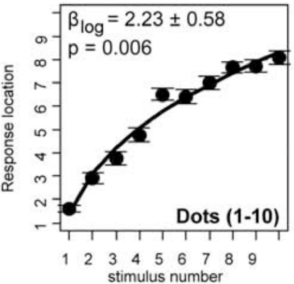
The elementary counting of dots by less numerate agents (e.g., children or indigenous people [8,9], Figure 2) presents a case of the metrology of discrete counting as a typical ‘analytical’ or ‘sampling by variable’ procedure [11,12] (bullet 1 and bottom-left entry in Table 1).
This study of elementary counting has several advantages, including the opportunity of analysing the measurement response where the analytical measurand (quantity intended to be measured)—the number of dots ( 1 10 )—is
  • (i) known exactly;
  • (ii) Conceptually simple.
In fact, this elementary case can exemplify each of the elements of Table 1, as will be shown throughout this paper.
As the number of dots to be counted exceeds about 5 (the number of digits on one hand traditionally used by the agents for counting), each estimated count becomes successively in error [8] (Figure 2). Similar observations of limitations in counting ability can be found in children and educated adults when they are given only a limited time to perform each counting task. The initial ‘analytical’ scenario 1 is the estimation of the measurand: the quantitative number of a set of discrete objects (with the number of dots increasing from 1 to 10) in the data shown in Figure 2. A count of 5 dots, where perceived counts deviate substantially from the known, true number of dots, could be considered a ‘limit of detection’ as an analytical performance metric.
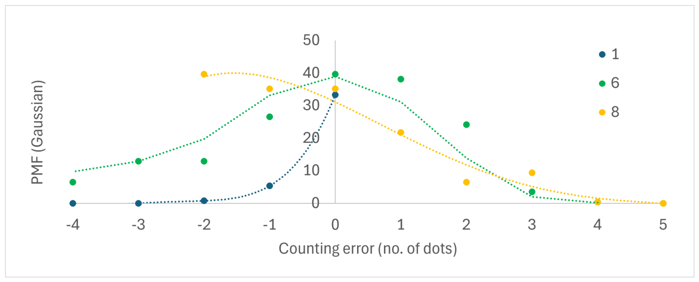
These successive count errors can be described in terms of PMFs distributed over an increasing number of counting categories, as shown in Figure 3. Analytical PMFs of distributions of perceived counting errors can be plotted, for example, for three counts: (1 dot, 6 dots and 8 dots) in the study [8] of elementary counting tasks (‘items’, j) of sets of clouds of increasing numbers of dots and task difficulty. The lines drawn for each count PMF assume a Gaussian distribution of counting error, p x = N ( ( μ μ 0 ) , σ 2 ) , μ   = perceived count, Equation (5); σ = 1 dot, perceived counting dispersion, Equation (6); μ 0 = true count.

4. Case Studies of PMFs: Quantitative Statistical Process Control

PMFs have been invoked for many decades for a number of well-known sampling distributions in the context of trials for statistical process control (SPC [36]) as one major area of application. In general, the parameters of a production process are unknown and can change with time. Procedures to estimate the parameters of probability distributions and solve other inference or decision-oriented problems related to them need to be developed. In this section, we will motivate how SPC PMFs can be deployed when tackling the metrology of clinical performance (Section 2), with a particular focus on the elementary counting example, Figure 2.

4.1. Binomial Distribution and Dichotomous Bernoulli Trials in SPC

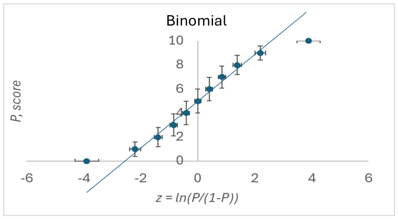
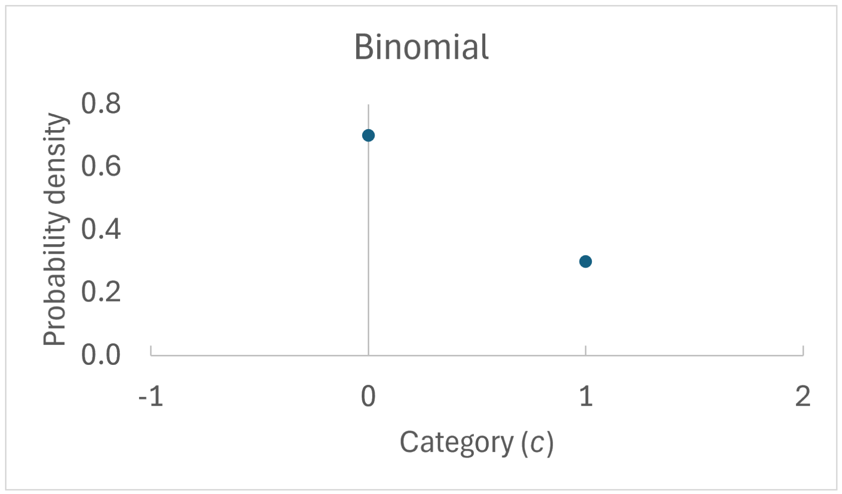
A basic kind of PMF is the dichotomous Bernoulli variant shown in Figure 4. For an elementary counting case, a counter may initially estimate the number of dots as one or another of two adjacent integers, say, ‘9’ or ‘10’ when counting a cloud of ten dots, corresponding to the top-left entry in Table 1.
For a dichotomous [38] ‘trial’, where a ‘success’ is scored 1 and a ‘failure’ 0, let the probability of categorising a ‘successful’ response be p. Values on the ordinate (vertical) axis of the binomial PMF shown in Figure 4 are probability density values:
P X ( x ) = P ( X = x c ) = c o u n t c N s a m p l e = i = 1 N s a m p l e [ z i = c ] N s a m p l e i f x R X 0 i f x R X .
On a quantitative scale on the abscissa, the PMF plotted in Figure 4 (based on Monte Carlo (MC) simulations of sampling trials [37]) has the mean and standard deviation p ^ = 0.5 , σ ( p ^ ) = 0.28 , while Equations (5) and (6) yield
p ^ = c = 0 c = 1 c · p c = 0.5
σ ( p ^ ) = c = 0 c = 1 ( c · p c p ^ ) 2 C 1 = 0.3 .
The binomial distribution is a limiting form of the Poisson distribution (Section 4.2) for an infinite number of Bernoulli trials and an infinitely small probability of non-conforming products [36].

4.1.1. Dichotomous Decision-Making with Uncertainty

A typical decision of conformity is whether the attribute of an entity (e.g., a product or sample) can be classified as above (‘positive’) or below (‘negative’) a specification limit, SL, for that quality characteristic. However, measurement uncertainty leads generally to the risk of incorrect decisions and classifications in such conformity assessments, as described in [17] JCGM 106:2012. As recalled in [4], in the context of laboratory accreditation with uncertainty, “Unlike ISO 17025, [39], ISO 15189 [40]…categorically requires the use of positive and negative samples (Point 7.3.4 letter f) for the uncertainty of qualitative results based on thresholds”.
An observed response in a performance test is typically scored binarily (binomial PMF, Figure 4) in one of two categories on the abscissa, as c = 1 for correct and as c = 0 for incorrect, and presented on the PMF ordinate as P s u c c e s s , i , j for each instrument, i, to a specific object, j, when examined in terms of Measurement System Analysis (Section 3.1). This simplest binary classification can be extended to polytomous decision-making over a range of classification categories (Section 4.2). In the elementary counting case, this would correspond to ‘guess-estimating’ the count to lie in a range of integer numbers of dots for a given cloud as an analytic measurand, as is evident in the results shown in Figure 3. A corresponding clinical performance study (Section 2) would identify two measurands: the (i) ability of the counter and the (ii) difficulty of each counting task derived from the probability of correct classification, corresponding, respectively, to the top-right and top-left entries in Table 1. In any case, the decision quandary reflects uncertainty. We share the views of Pradella [4], who writes: “‘doubt’ is not only a specialised concept in psychology [41], but a term of common language and everyday experience, attested in general vocabulary”, and which goes beyond the traditional ‘operational’ definition of ‘standard uncertainty’ as a standard deviation [42]. The next sections take this even further, by presenting psychometric modelling capable of dealing with the identification of performance measurands of ability and difficulty in the presence of uncertainty, culminating in the Rasch measurement model (Section 4.3) as a method of choice for the Metrology of Classification [43].

4.1.2. Distances on Categorical Scales: Counted Fractions

Distances on categorical scales, such as on a binomial PMF (Figure 4) (but also PMFs for other distributions, such as the Poisson and psychometric), can be challenging to evaluate correctly in the case of hidden, unrecognised non-linearity or simply a non-numerical scale (Section 2.1). This ‘scale ordinality’ obliges relatively more emphasis to be placed on the PMF ordinate values compared with more quantitative cases with PDFs such as the analytical (bullet 1). Typical clinical performance (bullet 2) cases include assessing the effects of an intervention or the relative performance of two counters (Figure 3) in terms of distances between PMFs.
As defined in Equation (4), the probabilities for the different categories of any PMF, c, P ( X = x c ) , must be non-negative and sum up to 1: P X ( x ) 0 and x P X ( x ) = 1 . A general feature of categorical data in which fractions on a finite scale are counted on any bounded scale is referred to as the ‘counted fraction’ effect [44]. Put simply, any score on a limited scale bounded by 0 and 100% becomes increasingly non-linear as either extreme of the scale is approached. A difference of, for example, 1% in a score P s u c c e s s of successful classification is a different amount at mid-scale (50%) compared with scores at 5% or 95%. This effect will be explained and compensated for as follows:
An early statement by Pearson [45] is given: “Beware of attempts to interpret correlations between ratios whose numerators and denominators contain common parts”.
The counted fraction effect has been explained in terms of the occurrence of the same term, Z j , in the numerator and denominator of the score Z j = Z j / ( k = 1 K Z k ) .
Tukey [44] wrote further: “As a general consequence we should expect that scales which have a finite range are likely to give us trouble unless all our observations tend to be safely away from any ends which are present. Hence the fact that percentages go only from one end (at 0%) to another (at 100%) suggests that, whenever even moderately extreme percentages are likely to occur, we are likely to have to ‘stretch the tails’, while, if really extreme percentages occur, we may have to stretch hard enough so that there are no ends (at any finite values).”
Filzmoser [46] stated for basically the same concept in the context of mineral compositional data studies: “If not all variables or components have been analysed, this constant sum property, (viz., x P X ( x ) = 1 (Section 2.1)) makes the relation between variables not ‘real’ but ‘forced’…For example, if the concentrations of chemical elements are measured in soil samples, and if an element like SiO2 has a big proportion of, say, 70%, then automatically the sum of the remaining element concentrations is at most 30%. Increasing values of SiO2 automatically lead to decreasing values of the other elements, and even if not all elements of the soil have been measured, the correlations will be mainly driven by the constant sum constraint.”
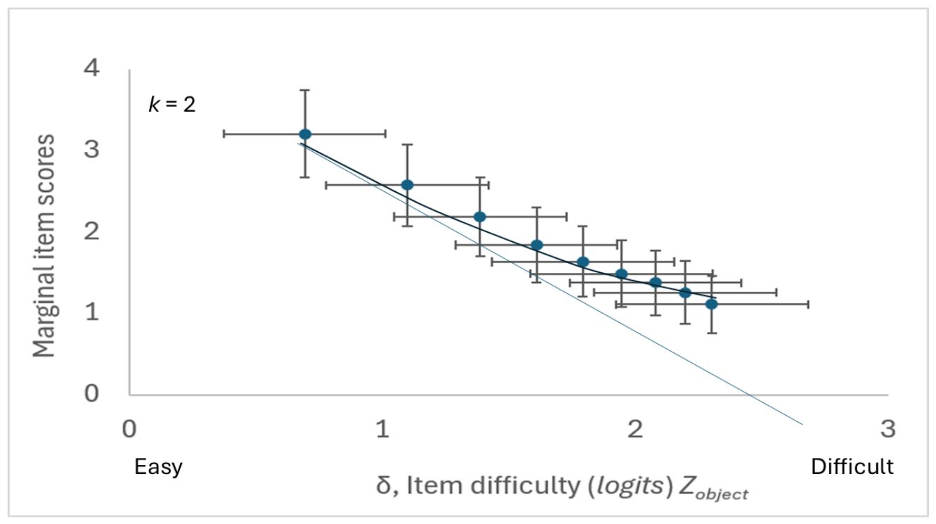
Non-linearity in the raw response scale, such as that which arises from the counted fraction effect [47], can be readily revealed by plotting, as in Figure 5 and Figure 6, the marginal probabilities for the different items j (cloud of dots to be counted, for example), given by Σ i = 1 N T P y i , j N T P , against the more quantitative scales from Rasch Measurement Theory (RMT) [48] for the task difficulties, δ j , (logits), as will be described below. As is clear from both figures and as expected from the counted-fraction effect, while substantially linear in the central region around 50 percent successful classification, there is increasing non-linearity towards the scale extremes (low scores in Figure 6 and for both low and high scores in Figure 5, exactly as said by Tukey [44]).
Scale non-linearity caused by the counted-fraction effect is ubiquitous to all PMFs because of the limited percentage scale (Equation (4)), but if not recognised (as in Classical Test Theory, CTT, [49] which is still widely used, even in the most recent literature [12]) it can lead to serious underestimation of true scores at either end of the response scale, as shown in Figure 5 and Figure 6, compared with the substantially linear region close to mid-scale (Equation (10) (Section 4.1.3)). Without compensation —”stretching the tails”, in the words of Tukey [44]—the counted-fraction effect will invalidate even the simplest mathematical and statistical expressions, such as those used when calculating an average or expressing a law of probability (Equation (1) in [12]).

4.1.3. Compensating for Counted-Fraction Scale Non-Linearity

There is a substantial and growing body of literature ([2], pp. 88–89) for a diversity of applications, such as psychometry [48] and compositional data analysis [46,50], where the counted fraction effect is recognised. The ‘counted fraction’ effect can be compensated for using a log-odds (GLMM) approach (Equation (11)):
Ordinate values compensating for the counted fractions effect are given as a straight line y = m · z + c , as plotted in Figure 5 and Figure 6, where two statistics are known:
  • The intercept c = 0.5 at z = 0 .
  • The slope.
    m = d p d z = p ( z ) · ( 1 p ( z ) ) = 0.25
    at z = 0 , p = 0.5 .
These two parameters, which apply to all bounded-scale fractions, define the anchor (at P s u c c e s s = 50%) and the span (the slope) of the linear, quantitative scale resulting from a log-odds transformation Equation (11), thus giving the corrections to raw performance data for the counted-fraction effect for any PMF.
Ordinality in responses generally compensates for the effects of counted fractions by taking log-odds ratios (ORs) [51], i.e.,
log ( O R ) = log ( x j 1 x j ) = z .
The RHS of Equation (11) is referred to as a ‘link function’ in the literature in the Generalised Linear Measurement Model (GLMM) approach [52] and provides the means for common-person and common-item equating in psychometrics, following Wright’s expansions of Rasch’s models ([53] pp. 109–117). For current application, see [54].

4.2. Poisson Distributions in SPC

The Poisson is another widely applied distribution used to model count data and random occurrences over time or space, such as arrivals in a queue, radioactive decay events or rare defects in SPC production [55]. We will also examine in (Section 4.3.3) how the Poisson distribution can be useful when defining clinical performance metrics for the elementary counting case (Figure 2).
Let λ denote the expected number of events per interval, and assume λ is known. Then, the distribution of X is Poisson with parameter λ :
X Poisson ( λ ) .
The PMF for X is
p X ( x ) = λ x e λ x ! , x = 0 , 1 , 2 , , 0 , otherwise .
X is the quality characteristic, x, being classified (e.g., number of defects) in n observations.
X has expectation and variance ([36], p. 55)
E ( X ) = λ , V ( X ) = λ .
The Poisson and binomial distributions are closely related: The Poisson distribution can be regarded as a limiting form of the binomial distribution (Section 4.1). Allowing the binomial parameters n and p 0 in such a way that n · p = λ results in a Poisson distribution [36]. According to Meredith [56], the Poisson distribution “also occurs as a limit distribution for a number of discrete distributions other than the binomial. Two of the more important instances of this are the negative binomial or Pascal distribution and the hypergeometric distribution.”
As for the binomial (dichotomous Bernoulli trials) case (Section 4.1), values on the ordinate (vertical) axis of the Poisson PMF are probability density values for each x:
p x = c o u n t x / N s a m p l e = i = 1 N s a m p l e [ z i = x ] / N s a m p l e .
On a quantitative scale on the abscissa, each Poisson PMF—plotted in Figure 7 for the elementary counting case—has the mean and standard deviation given by
p ^ x = x = 0 x = X x · p x ;
σ ( p ^ x ) = 1 / ( X 1 ) · x = 0 x = X ( ( x · p x p ^ x ) 2 ) .

4.3. Rasch Psychometric Model: Principle of Specific Objectivity

The output of the uncertainty model (Section 3.1) will ultimately provide (through ‘restitution’), from an MSA perspective (Figure 1), our best estimates of the instrument attribute (typically an ‘ability’ of a rater to make a ‘correct’ classification), alongside the object attribute, which together constitute a ‘conjugate’ pair of measurands. This procedure for clinical properties involving ordinal (and nominal) PMFs has the same role as the corresponding procedure for data on fully quantitative scales, when calibrating the sensitivity of, for instance, a weighing machine in order to metrologically determine the mass of an unknown weight. Providing separate estimates of measurement system attributes from the analysis of PMFs on the less quantitative scales will require dealing with possible scale non-linearity (Figure 6). Again, a psychometric model will be useful when defining clinical performance metrics for the elementary counting case (Figure 2) and corresponding to the top-right entry in Table 1.
Amongst a family of log-odds transformation models (through restitution from the ordinal or nominal response scores, Y = P s u c c e s s , of the measurement system), a particularly metrological approach is the psychometric [48] modern measurement (dichotomous) theory [43,58], as a special case of the log-odds (Equation (11)):
y i , j = P s u c c e s s , i , j = e ( θ i δ j ) 1 + e ( θ i δ j )
or in the form of the log-odds:
l n ( P s u c c e s s , i , j ( 1 P s u c c e s s , i , j ) ) = θ i δ j
This not only compensates for counted fraction non-linearity (Section 4.1.2) but also allows separate estimates by logistic regression of Equation (18) to the response data (often using a maximum likelihood criterion) of the quantitative, continuous variables δ j —task difficulty of each set of objects, j—and θ i —agent ability of each of the set (‘cohort’) of instruments, with i as the principal clinical measurands, for instance, in our elementary case. (Note that this logistic regression is made on the whole matrix of responses of i instruments and j objects similar to, for instance, a least-squares subdivision, as opposed to bilateral, pairwise comparisons more commonly found in metrology (Section 4.1.1 in [2])).
The principle of specific objectivity is one major approach to providing separate estimates of these attributes as measurands [48]. Following the Principle of Specific Objectivity, MSA responses are not measures of the instrument’s (classifier’s or decision maker’s) ability, nor the classification task (object) difficulty, but they depend on both. Rasch [48] attempted to motivate his principle by drawing analogies to relations between several variables and the universal equations of Physics (such as Newton’s second law).
The MSA approach of engineering metrology is felt to be a closer point of departure [43] (Section 3.1). In accordance with Rasch’s principle of specific objectivity, task difficulty and agent ability need to be treated separately:
  • ‘Agent’ ability, θ .
  • ‘Task’ difficulty, δ .
In making separate estimates of the measurands, ability and task difficulty, following the Principle of Specific Objectivity, when reliability and validity are to be assessed, the normal rules of statistics apply, as well as more metrological requirements, which go beyond requiring mere numbers to making judicious and representative sampling across the full range of measurement scales (Section 5.5).
Alongside his better-known log-odds expression (Equation (17)), the Poisson PMF distribution (Figure 7) of SPC was chosen by Rasch [57] when originally proposing his psychometric approach (Section 4.3.3) to determine the ability of individual cohort members to perform psychometric tests, such as reading. Misreadings in such tests correspond with the typical application of the Poisson distribution (Section 4.2) in quality control as a model of the number of defects or non-conformities that occur in a ‘unit of product’ [36]. In Rasch’s psychometric models [48,57], the Poisson rate factor λ = k / h , where ‘task’ difficulty, δ = l o g ( k ) , and ‘agent’ ability, θ = l o g ( h ) [59,60], are recognised as “a necessary condition for specific objectivity of comparisons between tests and between students”, with “the result that for the Poisson distribution the multiplicative structure (IX:2) of its parameter A is both necessary and sufficient for obtaining specific objectivity can be extended to the whole class of additive exponential models….” ([48], p. 92). How the Poisson distribution can be useful when defining clinical performance metrics for the elementary counting case (data shown in Figure 2), particularly the case in the top-right cell of Table 1, is further examined in (Section 4.3.3).

4.3.1. Agnostic Rasch Models

Most applications of Rasch’s measurement models [48,57] have to date been made in education, health care, and survey research, involving persons who act as instruments [43], such as in the elementary counting example (Section 5). But that model is not mathematically limited to psychometrics or human respondents but should also be applicable to more technical agents, as Rasch [61] recognised in his retirement lecture, which he closed by saying that the potential for use of the models he developed “stretches to all sciences where the subjects are comparisons that must be objective”.
Diverse examples include
  • A material hardness indenter [62] to make an impression (JCGM VIM [63] EXAMPLE 1 Rockwell C hardness);
  • A hospital to provide a service (A & E [64], surgery [65]);
  • In psychophysics, that is, where various physical fields and forces impinge on the five senses of an agent [43,66].
These cases are amenable to an analysis in terms of the following measurands: (i) an ‘ability’ of an agent and the ‘difficulty’ of a task, or, alternatively, (ii) in usability studies [67], the ‘leniency’ of an agent and the ‘quality’ of a product or service, by exploiting the agnostic aspect of the Rasch measurement model (Section 4.3).

4.3.2. Polytomous Measurement Models

Rasch’s dichotomous measurement model version (Equation (17)) has subsequently been complemented by the corresponding polytomous measurement model variants as well as multilevel [68,69], multidimensional [70], multifaceted [71,72], mixture [73], and other models. As an example, JCGM VIM [63] EXAMPLE 4, Subjective level of abdominal pain on a scale from zero to five, belongs here.
Registering the response, P s u c c e s s , of the measurement system when instrument resolution is limited or levels of uncertainty are high in the measurement process is often made more practically in terms of a Probability Mass Function (PMF) with discrete categories rather than as a continuous response scale (so-called ‘visual (analogue) score’) by rounding off to the nearest integer, even when the object quantity varies on a continuous scale.
Polytomous classification is the term used when more than two categories are assigned. In the elementary counting case, Figure 2, this would correspond to ‘guessing’ the count to lie in a range of integer numbers of dots for a given cloud, as a clinical performance study (Section 2). There is an extensive body of literature—for instance, in the educational assessment field [74]—where guessing can be modelled in much the same way as the MSA approach (Section 3.1); in classical measurement, engineering parametrises measurement errors such as bias.
Approaches to polytomous response analysis include the so-called ‘partial credit model’ (PCM [75,76]) in which the binary (dichotomous) log-odds ratio (OR) models are extended to polytomous cases, as summarised as follows:
Probability q i , j , k of response x i , j of instrument (agent) i, object (item) j, over k categories for the PCM:
q i , j , k = exp c = 0 k ( θ i δ j , c ) exp k = 0 C j · ( c = 0 k ( θ i δ j , c ) ) .
An alternative to the PCM is the Rasch Rating Model [77]:
P r ( Y i , j = q ) = q i , j , k = exp c = 0 k ( θ i δ j , c τ c ) exp k = 0 C j · ( c = 0 k ( θ i δ j , c τ c ) )
where τ c is the threshold of category c.
This formalism applies even in the present case of elementary counting, where, for each task of counting a number of dots, an individual cohort member is making a polytomous decision: “how many dots do I see?” among the set of potential dot numbers (Section 4.3.3).

4.3.3. Poisson PMFs for Counting

At about the same time as Rasch [48] formulated his psychometric model (Equation (17)), he also considered [57] an alternative formulation referring to a probabilistic Poisson distribution (Section 4.2) well known from SPC as a model of the number of defects or nonconformities that occur in a unit of product when classifying it:
p ( x ) = e λ λ x x ! ; x = 0 , 1 , , n
where x is the ‘quality characteristic’ being classified (number of defects) in n observations.
The rate parameter λ is equal directly both to the mean and variance of the Poisson distribution ([36] p. 55 and (Section 4.2)). In [57] a Rasch Poisson PMF was given as a model for the number of ‘misreadings’ by a child (i) for a text (j) of a particular level of difficulty. As quoted in [60], and references therein: “Although it is one of the earliest models that Rasch has developed, the Rasch Poisson Counts Model has received less attention than other binary or polytomous Rasch models”.
A much earlier observation by Meredith [56] noted: “a thorough understanding and application of such a particularly simple [Poisson] model is often the key to further development of suitable stochastic models in scientific work”.
The fundamental value obtained via the Poisson counts model was only belatedly realised by Rasch ([78] p. 66) when, after a 1959 conversation with a colleague, he suddenly realised “that the possibility of separating two sets of parameters must be a fundamental property of a very important class of models,” and that his study of children’s misreadings had led him to devise a new “class of probability models [having] the property in common with the Multiplicative Poisson Model, that one set of parameters can be eliminated by means of conditional probabilities while attention is concentrated on the other set, and vice versa.” Andrich [79] then showed that the Poisson distribution is necessary and sufficient for constructing measures from discrete observations.
In the present work, the example of the elementary counting of dots, akin to the Rasch [57] counting study, not only provides an ‘analytical, sampling by variable’ PMF (Section 3.3) but will also exemplify how Poisson PMFs can be benchmarked against full psychometric studies as ‘clinical, sampling by attribute’ PMF studies (Section 5).
In the case study of dot counting by the Munduruku (indigenous people of Brazil) [8,9], Poisson PMFs, as ‘clinical’ cases in the top-left cell of Table 1, can be derived with Equation (21) since task difficulty can be calculated from first principles (Equation (26)), from the number of dots being counted, thanks to the conceptual simplicity of the task [80] (p. 66ff). Table 2 shows the PMF values from the Poisson rate, λ , calculated by entering the simulated counting difficulty δ into Equation (21), where k j = e δ j and taking a cohort-average ability, θ m e a n , yields h i = e θ i .
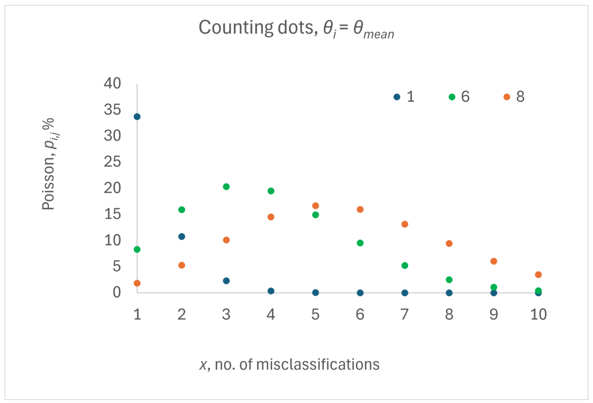
Figure 7 shows the resulting plots of PMFs for three cases (true counts of dots: (1), (6) and (8)). These PMFs show the distribution of probabilities for each object count (no. of dots), with a shifting maximum—e.g., at x = 5 misclassifications for eight dots—corresponding to the most likely value of x, the quality characteristic being classified (number of misclassifications) in n observations, where those miscounts are those shown in the analytical plot of Figure 3.
  • In contrast to Rasch’s [48] psychometric model, it is important to note that Poisson [81] placed important restrictions on the applicability of his model: particularly that the mis-classification events were to be “very rare”, as should apply to the PMFs shown in Figure 7. Although there appears in the literature to be no exact threshold where the Poisson approximation breaks down, a ‘rule of thumb’ is as follows: λ = n · p is moderate (typically n · p 5 10 for good accuracy) (Figures 2–24 in [36]). Our psychometric simulations (Section 5) of task difficulty and counter ability do not suffer from the same restrictions and allow the choice of response level, P s u c c e s s , over a complete range (shown later in Figure 9): from the most mis-classifications (for a low-ability counter attempting a difficult counting task) to the least number of mis-classifications, where the Poisson approximation should be valid in the latter case (i.e., for a high-ability counter performing an easy counting task) [82]. The Poisson ‘rule of thumb’ range can be seen to be comparable with the mis-classification rates shown in Figure 7. However, to make a full comparison between the classic ‘rule of thumb’ limit to the Poisson distribution and the present psychometric simulations requires a proper account of the applicability of the ergodic principle: that is, to what extent the classic group-statistic Poisson approach [36,81] corresponds to the individual statistics of Rasch [57] psychometric modelling. For instance, the Poisson rate λ = n · p has in some way to be interpreted in psychometric cases where n = 1 , i.e., just one counting agent (MSA: Instrument), while, at the same time, the overall number of degrees of freedom needs to be sufficiently large to achieve adequate reliability and validity (Section 5.5).
  • The Poisson PMF number of mis-classifications shown in Figure 7 has no information about which numbers are perceived correctly or not, but should in principle correspond—for each item (j)—to the occupancies of the analytical PMFs shown in Figure 3. Similarly, the Poisson PMF number of mis-classifications has no obvious relation to the corresponding ‘clinical’ metrics, that is, the counting task difficulty and the counter ability. (In principle, one can estimate the expected count by inverting Equation (21) since—in the present case of an elementary construct—the relation between task difficulty and the number of dots is known (Equation (26))). Future work is intended on this novel approach to benchmarking of the Rasch Poisson Counts Model against full psychometric Rasch modelling, as mentioned in the final Discussion (Section 6).

5. ‘Clinical’ Psychometric Study: Counting Dots

The elementary counting of dots by less numerate agents (e.g., children or indigenous people [8,9]) (data shown in Figure 2) also presents a case typical of the metrology of counting as a ‘clinical’ or ‘sampling by attribute’ procedure (Section 2) corresponding to the top row of Table 1, as follows.

5.1. Dichotomous and Polytomous Mis-Classification Probabilities. CTT and Rasch Measurement Theory

Regularly used clinical performance metrics (Section 2) of measurement systems include: ‘sensitivity’ (Equation (22)) and ‘selectivity’ (Equation (23)), which are plotted against each other on receiver operating characteristic curves [33], when sampling by ‘attribute’, and are often analysed with CTT despite its known limitations (Section 4.1.2).
Dichotomous mis-classification probabilities [83,84] due to binary decision quandary arising from uncertainties are
  • F A P = P [ Y = 1 | X = 0 ] ; False Acceptance (or positive, FPR) Probability;
  • F R P = P [ Y = 0 | X = 1 ] ; False Rejection (or negative, FNR) Probability.
These two probabilities lie on the off-diagonal of a 2 × 2 decision matrix for a binary test, where the true positive and true negative classification probabilities lie on the diagonal. Each pair of probabilities—positive (TP, FP) and negative (FN, TN)—can be plotted as binary PMFs, like the binomial plots shown in Figure 4.
Performance metrics can be defined for the case of a binary decision A or B about an entity when assessed for conformity with respect to a specification limit, SL, for the quantity, z, of interest, based on a signal (SN with noise) in the presence of noise, N [33]:
True positive rate (TPR), a.k.a. sensitivity or recall:
P ( A S N ) = z > S L N z , detected z N z , detected .
True negative rate (TNR), a.k.a. selectivity (or specificity in clinical/diagnostic contexts):
P ( B N ) = z < S L N z , not detected z N z , detected .
The elementary counting case, Section 5, corresponds to a polytomous extension (Section 4.3.2) of each of these classic clinical performance metrics.
Recall that “clinical performance aims to demonstrate that the measurement instrument can achieve clinically relevant outputs through predictable and reliable use by the intended users”, scenario 2 [29]. Considering the known (but not always recognised) limitations in CTT (Section 4.1.2), a more reliable approach to clinical performance assessment [35,85,86,87] is therefore to deploy Rasch Measurement Theory (Section 4.3), which:
  • (i) Compensates for counted-fraction scale non-linearity (Section 4.1.3);
  • (ii) Exchanges the analytical measurands (such as the number of dots, Section 3.3) for the clinical measurands: counting task difficulty and counter ability.
In the ‘clinical’ scenario 2, the level of difficulty attributed to each object counted and the ability attributed to each counter (the person or, in MSA terms 1, the ‘instrument’) both contribute in some way to the probability of successful counting. For a proper metrological analysis of the clinical analysis of counting, PMFs (occupancy: probability of responses in each category (number of dots)) for a range of tasks of increasing levels of difficulty can be analysed psychometrically, where the quantities (measurands) of interest are primarily the ability of each counter and the level of difficulty of a certain number of dots (rather than the actual number of dots—which of course can be determined by any capable counter).

5.2. Counted-Fraction Scale Non-Linearity When Counting Dots: ICC

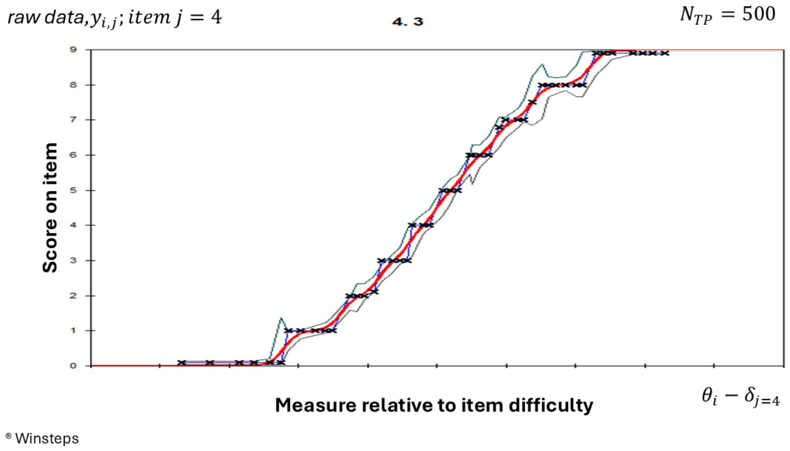
Figure 8 exemplifies for the elementary counting case (Section 5) a so-called ICC (Item Characteristic Curve [88]) for a particular item, calculated for a selected counting task (difficulty δ j , j = 4 ), using PCM modelling of polytomous data distributed across a cohort of test agents (persons counting) calculated as follows:
Figure 8. ICC (red, solid line)—together with upper and lower confidence intervals (grey, solid lines above and below) from logistic regression) of partial credit model (Equation (19), to polytomous data (crosses), 10 categories, 0 , , 9 ) to raw scores on the y-axis; calculated with the Rasch formula for P s u c c e s s , i , j (Equation (17)) across a simulated cohort of varying (x-axis) counting ability, θ i , for a selected counting task (difficulty δ j , j = 4 , shown in Figure 9) of elementary counting tasks (‘items’, j) of a set of clouds of increasing number of dots 1 , , 10 [8] ( N T P = 500 ) .
Foundations 06 00026 g008
For an item with categories c = 0 , 1 , 2 , , k and Andrich thresholds τ c (Equation (20)), with τ 0 chosen to be 0, the following holds: At location x on the latent variable (relative to the item difficulty), the probability of observing category c is P c ( x ) = e c · x c = 0 k τ c s u m p ( x ) , where s u m p ( x ) = c = 0 k e c · x s u m ( τ c ) for c = 0 to k. The expected score y at location x is given by y = c = 0 k ( c · P c ( x ) ) .
Further publications referring to the simulation of psychometric ICC models can be found in, for example, [89,90]. In the present work, the simulated values as described in (Section 4) simply use the usual dichotomous Rasch expression (Equation (17)) (which for benign data sets should give at least as good estimates as rounding to the nearest category, c, as described by [90]).

5.3. Communication of Measurement Information Throughout the Measurement Process: Amount of Entropy

To meet the challenge posed by PMF axes being often on less quantitative or even nominal scales, where even the most basic arithmetic operations cannot be assumed to always work (Section 4.1.3), a viable alternative to calculating distances (even on ordinal and nominal scales) of PMF plots is to take differences in informational (Shannon) entropy.
The amount of measurement information on the categorical scales of signals in each classification category, c, at any one point and state in the measurement process (from object, through instrument and operator to restitution (Figure 1) can be expressed as a [91] ‘surprisal’ l n ( q c ) , while the relative contribution to the total entropy is weighted with the relative occupancy, qc (chapter 5 in [2]).
The propagation of measurement information depicted in Figure 1, where information can be lost, distorted or gained, is described more readily with sums and differences of informational entropy than with the corresponding combination of probabilities and PMFs. An example of additions of entropy is found in the so-called Mutual information: I ( Z ; Y ) = H ( Z ) H ( Z | Y ) , which has been used by Benish [92], where an individual’s disease state is denoted Z while the diagnostic test result is Y. The well-known Kullback–Leibler (K-L) metric d K L ( P , Q ) for a response Y, PMF Q ( y ) , to an object attribute Z, PMF P ( z | A ) , is
d K L ( P , Q ) = z · d P s u c c e s s = [ P s u c c e s s · l o g ( P s u c c e s s ) + ( 1 P s u c c e s s ) · l o g ( q P s u c c e s s ) ] = H ( P , Q ) H ( P ) .
The K-L parameter, Equation (24), is admittedly a valid metric only for infinitesimally small distances and is only one of several candidates for PMF distance metrics widely used, for example, in automatic image classification [93]. It can also be shown (Section 5.5.3 in [2]) that log-odds transformed data correspond to entropy (Equation (11)).
The start of the measurement process has a deficit in overall entropy (that is, the amount of ‘useful’ measurement information initially available), which, for a discrete PMF, is Δ H ( P ) = k p k · l n ( p k ) , where p k is the occupancy of category k from the actual quantity attributed to the measurement object. For conceptually simple tasks—such as the counting of dots—this calculated entropy will provide a metrological reference for calibration of classification properties, as illustrated in the current case study (Section 5.4.1). From a measurement system perspective, the response of the instrument (often a score, P s u c c e s s , made by a ‘rater’) will provide an input, X 1 , when establishing the measurement result (Section 3.1).

5.4. Simulated PMFs for the Elementary Counting Case

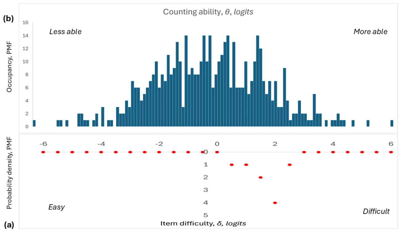
PMFs are shown in Figure 9 for simulated data for a set of clouds of dots (of increasing (a) (red histograms) task (’object’) counting difficulty, based on entropy theory (Equation (26), Section 5.4.1) and (b) (blue histograms) counter ability (Section 5.4.2), as the conjugate pair of psychometric measurands [8,9]. The blue bars in Figure 9b illustrating the occupancy PMF indicate the numbers of persons at that logit θ value, and the red dots in Figure 9a indicate the number of items at the corresponding logit δ values. When θ and δ are equal (vertically aligned), the logit difference between them is 0, and the success odds are 50–50. The odds of success increase the further to the right a blue bar is in relation to a red dot, as the positive difference between θ and δ grows. Conversely, the further to the left a blue bar is in relation to a red dot, the lower the odds of success become, and the differences between θ and δ become negative.

5.4.1. Counting Task Difficulty Simulated: Object (Task) Entropy

For the present guide on PMF simulations, ‘seed’ values will be considered in a study of elementary counting (of dots by Munduruku indigenous people in Brazil, [8]). A set of clouds of dots was presented visually for each counter as a sequence of counting tasks (‘objects’). Task difficulty is in general proportional to entropy—a more ordered (less entropy) task is easier to perform [80,94].
For the current purpose of demonstrating best practice when simulating uncertainties associated with PMFs, of particular interest will be cases where attributes—for instance, the level of difficulty of tasks—are sufficiently simple conceptually so that simulations can be ‘seeded’ with realistic start values. Beyond numerical simulation, it will be particularly valuable if ab initio estimates of categorical quantities such as task difficulty are available. Recent work has demonstrated how such knowledge-informed seed values can indeed be calculated even for categorical properties in a manner analogous to establishing metrological reference values in the more quantitative metrology in chemistry and the material sciences, as demonstrated in the neurodegeneration studies of legacy memory tests [95], where recall task difficulty could be expressed with the so-called Construct Specification Equation (CSE [96,97,98,99]):
δ = Σ k β k · Z k
in terms of entropy-based explanatory variables  Z k . The PMFs plotted (red histograms) in Figure 9 against the measurand, counting task difficulty, δ j , are those predicted to increase discretely, reflecting the increasing number, G, of integer dots in successive clouds according to the basic Hartley entropy [100]:
δ j = l n ( G j )
assuming a random distribution of identical dots in each cloud counted. (The addition of some symmetry to a cloud of dots would make the counting task easier, in terms of a lowering in the overall task entropy, as has been studied for elementary memory recall tests [80], p. 68.)

5.4.2. Counting Classifier Ability Simulated

  • Excel:
    N O R M . I N V ( R A N D ( ) ; 0 ; 2 )
    returns a vector of random numbers having the Normal distribution of the measurand counter abilities across the cohort shown with the blue histograms in Figure 9.

5.5. Reliability and Validity

In making separate estimates of the conjugate attributes, δ j and θ i —which are not merely the measurands, but also for ‘clinical’ purposes the quality characteristics, when conformity assessment is made—the normal rules of statistics of course apply—including making sufficient numbers of observations of items and instruments—to ensure minimum levels of reliability and power, as these are relevant in fit-for-purpose designs distinguishing between the varying demands of screening, diagnostic, accountability, and research applications. Additional, more metrological requirements go beyond requiring mere numbers to making judicious and representative sampling across the full range of measurement scales. For metrological purposes—concerning both precision and trueness (for metrological invariance, comparability and interoperability)—the underlying scale needs to be unidimensional, linear, quantitative, well targeted, free of differential item functioning, etc., and there is a whole battery of conventional tests of model validity [94].
The standard uncertainty in the ‘height’ (i.e., occupancy, P s u c c e s s ) of a PMF column is
u ( P s u c c e s s ) = P s u c c e s s · ( 1 P s u c c e s s ) n ,
derived from the underlying binomial distribution (Equation (7)). One should, however, always respect the inherent non-linearity of the scale, such as due to the counted-fractions effect (Section 4.1.2). A more proper estimation of this uncertainty is to first calculate the uncertainties in the link function, as given by the GLMM log-odds approach (Equation (11)).
Uncertainties (so-called Standard Errors, SE, i.e., standard uncertainties) in Rasch analyses with the logistic regression (Equation (18)) are those quoted by the WINSTEPS® program (section 21.120), where, according to that program’s manual (p. 805),
S E ( θ i , δ ˜ ) = 1 Σ j = 1 N i t e m s P s u c c e s s , i , j · ( 1 P s u c c e s s , i , j )
and
S E ( θ ˜ , δ j ) = 1 Σ i = 1 N T P P s u c c e s s , i , j ( 1 P s u c c e s s , i , j ) .
Thereafter, one can apply the inverse of the Rasch transformation in case the end-user wants to relate to the original PMFs. (Uncertainty intervals in P s u c c e s s calculated in that way will become increasingly asymmetric the closer the score is to either end of the scale, which is how it should be due to the counted-fractions effect.)
Reliability means assessing the influence of measurement uncertainty as an estimate of limited measurement quality. In psychometrics [53], a reliability coefficient, R β , for a Rasch variable β = β + ϵ β (for either Rasch attribute: β = θ or δ ), including an error term, ϵ β , is defined as
R β = var ( β ) var ( β ) = var ( β ) var ( ϵ β ) var ( β )
where the ‘true’ variance is v a r ( β ) and the observed variance is v a r ( β ) .
The consequences of the decisions to be made determine what the actual limits of reliability are, for instance, by setting a maximum permissible uncertainty. Traditional psychometric limits for so-called ‘high-stakes’ decisions are typically R β > 0.8 (Equation (31)), which corresponds to at most half of the observed dispersion being assigned to measurement uncertainty.

5.6. Validation of Simulated Logistic Regressions

The results of logistic regressions of the partial credit model (Equation (19)) to raw scores (y-axes of Figure 8; calculated with the dichotomous Rasch formula for task difficulty δ j , Equation (17)) across a simulated cohort of varying (x-axes) counting abilities, θ i , (Figure 9b) for a pair of selected counting tasks (difficulties δ j shown in Figure 9a) of elementary counting tasks, are presented. Using the WINSTEPS® program for this logistic regression, the raw scores were coded into categories by integer rounding of the % scores, as is particularly evident in the steps shown in Figure 8.
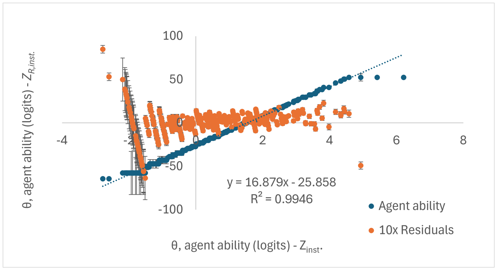
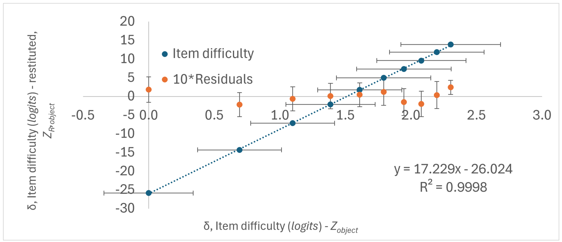
The validity of this procedure is investigated in Figure 10 and Figure 11 by comparing the restituted estimates (y-axes) of δ and θ with the original simulated values (x-axes) plotted, respectively.
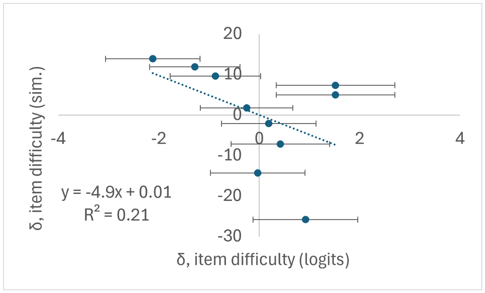
A second validation was made by comparing (Figure 12) simulated (y-axis) and original experimental data (x-axis) counting task difficulties from psychometric analysis (Rasch Equation (17)).

6. Discussion and Conclusions

The choice of construct—quantities attributed to an elementary counting process—in the current case study is made deliberately. The conceptual simplicity ensures the unidimensionality required in metrological psychometrics [48,94,101]. Additionally, it offers the opportunity to define—from first principles—metrological references (’gold standards’) [80] for counting task difficulty in terms of Construct Specification Equations [96,97,98,99,102] with explanatory variables based on informational entropy [103,104], as demonstrated in the simulation of counting task difficulty (Section 5.4.1). Such metrological references for calibration of categorical properties in turn enable interoperability and defining limits on quality of products and services of all kinds. (Other explanatory approaches beyond CSE include [105,106].)
This conceptual simplicity facilitates contrasting the metrology of three kinds of probability mass functions (PMFs) (Table 1) presented in this work: (i) quantitative response to a discrete range of counts (Figure 3); (ii) the classic Poisson distribution of miscounts (Figure 5); and (iii) psychometric (Rasch) distributions of counting task difficulty and person counting ability (Figure 9). New insights are provided when benchmarking the Rasch Poisson Counts Model (Section 4.3.3), which has received less attention, against full psychometric Rasch modelling (Section 5). Limits (traditionally rules of thumb on small probabilities and a large number of observations) on the validity of the Poisson distribution can be tested with access to psychometric simulations across the full range of task difficulty and counter ability.
A human being acting as a counter (MSA: A human as a Measurement Instrument [43]) is a prototype for more advanced applications, including counting, decision-making and similar classification tasks performed by Artificial Intelligence agents [7,43,80,107,108,109]. Logistic regression (Section 4.3) provides an essential complement when handling discrete and sometimes qualitative observations, in particular classifications [43], for example, to a typical use of Machine Learning in metrology where traditionally regular regression tasks are made on a continuous quantity [110]. The proposed methods will be useful when the traditional role of Physics in metrology is to be complemented by a typical ‘turn-of-the-millennium’ focus on the new metrology of ‘clinical’ and other applications where meaning and value, and not just numbers and analytics, are sought.
Future work is needed to extend the present studies to include less elementary and more complex constructs. There is much current research addressing multidimensional measurement theory and related topics in this field [35,111,112,113,114].

Author Contributions

Conceptualisation, L.R.P. and W.P.F.J.; methodology, L.R.P. and W.P.F.J.; validation, L.R.P. and W.P.F.J.; writing—original draft preparation, L.R.P.; writing—review and editing, L.R.P. and W.P.F.J. All authors have read and agreed to the published version of the manuscript.

Funding

RISE, through its internal programme supporting a Competence platform for categorical measurements, has provided funding for this work. Earlier research from European projects has also contributed, with support from the EMPIR programme, co-financed by the Participating States and from the European Union’s Horizon 2020 research and innovation programme, under grant numbers 15HLT04 NeuroMET and 18HLT09 NeuroMET2.

Data Availability Statement

All original measurement data come from [8]. Simulated data are produced in this work as described.

Acknowledgments

The authors thank members of the Joint Committee for Guides in Metrology (JCGM), Working Group 1 Guide to the Expression of Uncertainty in Measurement, for useful discussions.

Conflicts of Interest

The first author Leslie Pendrill was employed by the Swedish national metrology institute at RISE Research institutes of Sweden. William P. Fisher, Jr., is self-employed. Both authors declare that the research was conducted in the absence of any commercial or financial relationships that could be construed as a potential conflict of interest.

Glossary of Symbols

Explanation
discrete random variableX
range R X
event, category c A = X = x c
probability of X = x P X ( x )
probabilities for different categories, c P ( X = x c ) = N c / N S
occupancy of bin for category c N c
difference between the perceived and true dot count μ μ 0
true value, e.g., number of dots μ 0
dispersion, e.g., in number of dots σ
measurement object (MSA)entity, A
instrument (MSA)B
operator (MSA)C
object measurandZ
responseY
restitution via uncertainty modelR
object (A) probability of attribute z P ( z ; A )
response (y; z) probabilityQ = P ( y z ; A )
entropyH
Kullback–Leibler (K-L) metric d K L ( P , Q )
calibration function
relates the instrument response to the input
from the measurement object
f
“… focuses on the gathering of evidence
that the measurement instrument in question
reliably, accurately and consistently measures
and or detects an analyte” [29].
analytical performance
“…aims to demonstrate that the measurement
instrument can achieve clinically relevant outputs through
predictable and reliable use by the intended users” [29].
clinical performance
log-odds ratio l o g ( O R )
expected number of events per interval  λ
expectation of Poisson distributionE(X) = λ
variance of Poisson distributionV(X) = λ
sample size N s a m p l e
ordinal or nominal response scores Y = P s u c c e s s
probability of response x i , j of instrument (agent)
i; object (item) j, over k categories
P r ( Y i , j = q ) = q i , j , k
False acceptance (or Positive, FPR) Probability F A P = P [ Y = 1 | X = 0 ]
False rejection (or Negative, FNR) Probability F R P = P [ Y = 0 | X = 1 ]
True positive rate (TPR) a.k.a. sensitivity P ( A S N )
True negative rate (TNR) a.k.a. specificity P ( B N )
probability of observing category c P c ( x )
probability of successful classification per category/class P success
instrument ability, (standard) uncertainty θ , u( θ )
task difficulty, (standard) uncertainty δ , u( δ )
explanatory variables Z k
number of, e.g., integer dotsG
Standard Error, i.e., standard uncertainty S E
reliability coefficient for a Rasch variable β = β + ϵ β ,
(for either Rasch attribute: β = θ or δ )
including an error term, ϵ β
R β

Abbreviations

The following abbreviations are used in this manuscript:
CTTClassical Test Theory
EMPIREuropean Metrology Programme for Innovation and Research
EPMEuropean Programme for Metrology
FAPFalse acceptance probability
FRPFalse rejection probability
GLMMGeneralised Linear Measurement Model
GUMGuide to the expression of uncertainty of measurement
ICCItem characteristic curve
IRTItem Response Theory
JCGMJoint Committee for Guides in Metrology
K-LKullback–Leibler
MSAMeasurement System Analysis
PMFProbability Mass Function
PDFProbability Density Function
RISEResearch Institutes of Sweden
RMTRasch Measurement Theory
SEStandard Error
VIMInternational Metrology Vocabulary

References

  1. Bureau International des Poids et Mesures. The International System of Units (SI), 9th ed.; BIPM: Sèvres, France, 2019. [Google Scholar]
  2. Pendrill, L.R. Chapter 2. In Quality Assured Measurement—Unification across Social and Physical Sciences; Springer: Cham, Switzerland, 2019. [Google Scholar] [CrossRef] [Scilit]
  3. Fisher, W.P., Jr.; Pendrill, L. (Eds.) Models, Measurement, and Metrology Extending the SI: Trust and Quality Assured Knowledge Infrastructures; De Gruyter Series in Measurement Sciences; De Gruyter Oldenbourg: Berlin, Germany; Boston, MA, USA, 2024. [Google Scholar] [CrossRef] [Scilit]
  4. Pradella, M. Measurement Uncertainty: New Definition, Viewpoints, and Laboratories. Laboratories 2026, 3, 4. [Google Scholar] [CrossRef] [Scilit]
  5. Fisher, W.P., Jr.; Massengill, P.J. (Eds.) Explanatory Models, Unit Standards, and Personalized Learning in Educational Measurement: Selected Papers by A. Jackson Stenner; Springer: Singapore, 2023. [Google Scholar] [CrossRef] [Scilit]
  6. Fisher, W.P., Jr. Measure and manage: Intangible assets metric standards for sustainability. In Business Administration Education: Changes in Management and Leadership Strategies; Marques, J., Dhiman, S., Holt, S., Eds.; Palgrave Macmillan: New York, NY, USA, 2012; pp. 43–63. [Google Scholar] [CrossRef] [Scilit] [PubMed]
  7. Barney, M.; Barney, F. Transdisciplinary Measurement through AI: Hybrid Metrology and Psychometrics Powered by Large Language Models. In Models, Measurement, and Metrology Extending the SI: Trust and Quality Assured Knowledge Infrastructures; Fisher, W.P., Jr., Pendrill, L.R., Eds.; De Gruyter Series in Measurement Sciences; De Gruyter Oldenbourg: Berlin, Germany; Boston, MA, USA, 2024; pp. 103–132. [Google Scholar] [CrossRef] [Scilit]
  8. Dehaene, S.; Izard, V.; Spelke, E.; Pica, P. Log or Linear? Distinct Intuitions of the Number Scale in Western and Amazonian Indigene Cultures. Science 2008, 320, 1217–1220. [Google Scholar] [CrossRef] [Scilit] [PubMed]
  9. Pendrill, L.R.; Fisher, W.P., Jr. Counting and Quantification: Comparing Psychometric and Metrological Perspectives on Visual Perceptions of Number. Measurement 2015, 71, 46–55. [Google Scholar] [CrossRef] [Scilit]
  10. Fisher, W.P., Jr. Bateson and Wright on number and quantity: How to not separate thinking from its relational context. Symmetry 2021, 13, 1415. [Google Scholar] [CrossRef] [Scilit]
  11. Helliwell, T.; Giles, T.; Fensome-Rimmer, S. ISO 15189:2012—An Approach to the Assessment of Uncertainty of Measurement for Cellular Pathology Laboratories; Guidance Document G146; The Royal College of Pathologists: London, UK, 2015. [Google Scholar]
  12. Pennecchi, F.; Bich, W. A Bayesian Model for Measurements by Counting. Qual. Quant. 2026. [Google Scholar] [CrossRef] [Scilit]
  13. Mallinson, T. Extending the justice-oriented, anti-racist framework for validity testing to the application of measurement theory in re(developing) rehabilitation assessments. In Models, Measurement, and Metrology Extending the SI; Fisher, W.P., Jr., Pendrill, L., Eds.; De Gruyter: Berlin, Germany; Boston, MA, USA, 2024; pp. 401–428. [Google Scholar]
  14. Sul, D.; Dominguez, D.G. Culturally responsive evaluation with Latinx communities through culturally specific assessment: Building the Latinx immigration trauma assessment. New Dir. Eval. 2024, 2024, 103–112. [Google Scholar] [CrossRef] [Scilit]
  15. Sul, D. Situating culturally specific assessment development within the disjuncture-response dialectic. In Models, Measurement, and Metrology Extending the SI; Fisher, W.P., Jr., Pendrill, L., Eds.; De Gruyter: Berlin, Germany, 2024; pp. 475–500. [Google Scholar]
  16. Sul, D.; Blackmon, A.T. Enacting culturally specific assessment by constructing a STEM leadership assessment framework. J. Educ. Meas. 2026, 63, e70048. [Google Scholar] [CrossRef] [Scilit]
  17. JCGM. Evaluation of Measurement Data—The Role of Measurement Uncertainty in Conformity Assessment; Technical Report JCGM 106:2012; Joint Committee for Guides in Metrology: Sèvres, France, 2012. [Google Scholar]
  18. Mitcham, C. (Ed.) Encyclopedia of Science, Technology, and Ethics; Macmillan Reference: New York, NY, USA, 2005. [Google Scholar]
  19. Andersen, E.B. Sufficient statistics and latent trait models. Psychometrika 1977, 42, 69–81. [Google Scholar] [CrossRef] [Scilit]
  20. Andrich, D. Sufficiency and conditional estimation of person parameters in the polytomous Rasch model. Psychometrika 2010, 75, 292–308. [Google Scholar] [CrossRef] [Scilit]
  21. Fischer, G.H. On the existence and uniqueness of maximum-likelihood estimates in the Rasch model. Psychometrika 1981, 46, 59–77. [Google Scholar] [CrossRef] [Scilit]
  22. Andrich, D. Distinctions between assumptions and requirements in measurement in the social sciences. In Mathematical and Theoretical Systems: Proceedings of the 24th International Congress of Psychology of the International Union of Psychological Science, Vol. 4; Keats, J.A., Taft, R., Heath, R.A., Lovibond, S.H., Eds.; Elsevier Science Publishers: Amsterdam, The Netherlands, 1989; pp. 7–16. [Google Scholar]
  23. Bhatt, U.; Antorán, J.; Zhang, Y.; Liao, Q.V.; Sattigeri, P.; Fogliato, R.; Melançon, G.G.; Krishnan, R.; Stanley, J.; Tickoo, O.; et al. Uncertainty as a Form of Transparency: Measuring, Communicating, and Using Uncertainty. In AIES ’21: Proceedings of the 2021 AAAI/ACM Conference on AI, Ethics, and Society (AIES ’21); ACM: New York, NY, USA, 2021; pp. 401–413. [Google Scholar] [CrossRef] [Scilit]
  24. ISO 5725-1:2023(en); Accuracy (trueness and precision) of measurement methods and results—Part 1: General principles and definitions. International Standard. ISO: Geneva, Switzerland, 2023.
  25. Brown, R.J.C.; Güttler, B.; Neyezhmakov, P.; Stock, M.; Wielgosz, R.I.; Kück, S.; Vasilatou, K. Report of the CCU/CCQM Workshop on ‘The Metrology of Quantities Which Can Be Counted’. Metrology 2023, 3, 309–324. [Google Scholar] [CrossRef] [Scilit]
  26. JCGM GUM. Joint Committee for Guides in Metrology – Part 6: Developing and Using Measurement Models; Number JCGM GUM-6:2020; JCGM: Sèvres, France, 2020. [Google Scholar]
  27. Rossi, G.B. Measurement and Probability: A Probabilistic Theory of Measurement with Applications; Springer: Dordrecht, The Netherlands, 2014. [Google Scholar] [CrossRef] [Scilit]
  28. Hofmann, B. “My Biomarkers Are Fine, Thank You”: On the Biomarkerization of Modern Medicine. J. Gen. Intern. Med. 2025, 40, 453–457. [Google Scholar] [CrossRef] [Scilit] [PubMed]
  29. European Commission. Factsheet for Manufacturers of In Vitro Diagnostic Medical Devices; European Commission: Luxembourg, 2020; Available online: https://health.ec.europa.eu/publications/factsheet-manufacturers-vitro-diagnostic-medical-devices_en (accessed on 13 February 2026).
  30. European Union. Regulation (EU) 2017/746 on In Vitro Diagnostic Medical Devices; European Union: Brussels, Belgium, 2017. [Google Scholar]
  31. ISO 3951-1:2022; Sampling Procedures for Inspection by Variables. International Standard. ISO: Geneva, Switzerland, 2022.
  32. ISO 2859-1:2026; Sampling Schemes Indexed by Acceptance Quality Limit (AQL) for Lot-by-Lot Inspection. International Standard. ISO: Geneva, Switzerland, 2026.
  33. Birdsall, T.G. The Theory of Signal Detectability: ROC Curves and Their Character; University of Michigan Library: Ann Arbor, MI, USA, 1973. [Google Scholar]
  34. Linacre, J.M. Bernoulli Trials, Fisher Information, Shannon Information and Rasch. Rasch Meas. Trans. 2006, 20, 1062–1063. [Google Scholar]
  35. Pendrill, L.R.; Melin, J.; Stavelin, A.; Nordin, G. Modernising Receiver Operating Characteristic (ROC) Curves. Algorithms 2023, 16, 253. [Google Scholar] [CrossRef] [Scilit]
  36. Montgomery, D.C. Introduction to Statistical Quality Control, 3rd ed.; Wiley: New York, NY, USA, 1996. [Google Scholar]
  37. NIST. Uncertainty Machine. Available online: https://uncertainty.nist.gov/ (accessed on 13 February 2026).
  38. Bernoulli, J. Ars Conjectandi; Opus posthumum; OCLC 7073795; Thurneysen Brothers: Basel, Switzerland, 1713. [Google Scholar]
  39. ISO/IEC 17025:2017; General Requirements for the Competence of Testing and Calibration Laboratories. International Organization for Standardization: Geneva, Switzerland, 2017.
  40. ISO 15189:2022; Medical Laboratories—Requirements for Quality and Competence. International Organization for Standardization: Geneva, Switzerland, 2022.
  41. Mari, L.; Brown, R.J.C.; Narduzzi, C.; Nordin, G.; Trapmann, S.; Varela Magalhães, D. What Is Measurement Uncertainty? A Discussion. Metrologia 2025, 62, 062101. [Google Scholar] [CrossRef] [Scilit]
  42. Joint Committee for Guides in Metrology. Evaluation of Measurement Data—Guide to the Expression of Uncertainty in Measurement; Technical Report JCGM 100:2008; JCGM: Paris, France, 2008; GUM 1995 with minor corrections. [Google Scholar] [CrossRef] [Scilit]
  43. Pendrill, L.R. Man as a Measurement Instrument. NCSLI Meas. 2014, 9, 24–35. [Google Scholar] [CrossRef] [Scilit]
  44. Tukey, J.A. Data Analysis and Behavioural Science. In The Collected Works of John A. Tukey, Volume III; Jones, L.V., Ed.; Chapman and Hall: London, UK, 1984. [Google Scholar]
  45. Pearson, K. Mathematical contributions to the theory of evolution: On a form of spurious correlation which may arise when indices are used in the measurements of organs. Proc. R. Soc. 1897, 60, 489–498. [Google Scholar] [CrossRef] [Scilit]
  46. Filzmoser, P.; Hron, K.; Reimann, C. Principal Component Analysis for Compositional Data with Outliers. Environmetrics 2009, 20, 621–632. [Google Scholar] [CrossRef] [Scilit]
  47. Wright, B.D. Thinking with Raw Scores. Rasch Meas. Trans. 1993, 7, 299–300. [Google Scholar]
  48. Rasch, G. Probabilistic Models for Some Intelligence and Attainment Tests; Danmarks Paedagogiske Institut: Copenhagen, Denmark, 1960. [Google Scholar]
  49. Andrich, D. Rating Scales and Rasch Measurement. Expert Rev. Pharmacoecon. Outcomes Res. 2011, 11, 571–585. [Google Scholar] [CrossRef] [Scilit] [PubMed]
  50. Aitchison, J. The Statistical Analysis of Compositional Data. J. R. Stat. Soc. 1982, 44, 139–177. [Google Scholar] [CrossRef] [Scilit]
  51. Bland, J.M.; Altman, D.G. The Odds Ratio. Br. Med. J. 2000, 320, 1468. [Google Scholar] [CrossRef] [Scilit] [PubMed]
  52. McCullagh, P. Regression Models for Ordinal Data. J. R. Stat. Soc. 1980, 42, 109–142. [Google Scholar] [CrossRef] [Scilit]
  53. Wright, B.D.; Stone, M.H. Best Test Design: Rasch Measurement; MESA Press: Chicago, IL, USA, 1979. [Google Scholar]
  54. Student, S.R.; Briggs, D.C.; Davis, L. Growth Across Grades and Common Item Grade Alignment in Vertical Scaling Using the Rasch Model. Educ. Meas. Issues Pract. 2025, 44, 84–95. [Google Scholar] [CrossRef] [Scilit]
  55. Montgomery, D.C.; Runger, G.C. Applied Statistics and Probability for Engineers, 5th ed.; John Wiley & Sons: Hoboken, NJ, USA, 2011. [Google Scholar]
  56. Meredith, W.M. The Poisson Distribution and Poisson Process in Psychometric Theory; ETS Research Bulletin Series RB-68-42; Educational Testing Service: Princeton, NJ, USA, 1968. [Google Scholar]
  57. Rasch, G. On General Laws and the Meaning of Measurement in Psychology. In Proceedings of the Fourth Berkeley Symposium on Mathematical Statistics and Probability, Volume 4: Contributions to Biology and Problems of Medicine; Neyman, J., Ed.; University of California Press: Berkeley, CA, USA, 1961; pp. 321–333. [Google Scholar]
  58. Fisher, W.P., Jr. Invariance and traceability for measures of human, social, and natural capital: Theory and application. Measurement 2009, 42, 1278–1287. [Google Scholar] [CrossRef] [Scilit]
  59. Bashkansky, E.; Turetsky, V. Ability Evaluation by Binary Tests: Problems, Challenges and Recent Advances. J. Phys. Conf. Ser. 2016, 772, 012012. [Google Scholar] [CrossRef] [Scilit]
  60. Liu, R.; Liu, H.; Shi, D.; Jiang, Z. Poisson Diagnostic Classification Models: A Framework and an Exploratory Example. Educ. Psychol. Meas. 2022, 82, 506–516. [Google Scholar] [CrossRef] [Scilit] [PubMed]
  61. Rasch, G. Retirement Lecture of 9 March 1972: Objectivity in Social Sciences: A Method Problem. Rasch Meas. Trans. 2010, 24, 1252–1272, Translated by Cecilie Kreiner. [Google Scholar]
  62. Stone, M.; Stenner, J. From Ordinality to Quantity. Rasch Meas. Trans. 2014, 27, 1435–1437. [Google Scholar]
  63. Joint Committee for Guides in Metrology (JCGM). International Vocabulary of Metrology—Basic and General Concepts and Associated Terms (VIM), 3rd ed.; JCGM 200:2008 with minor corrections (2012); Joint Committee for Guides in Metrology (JCGM): Paris, France, 2008. [Google Scholar]
  64. Pendrill, L.; Espinoza, A.; Wadman, J.; Nilsask, F.; Wretborn, J.; Ekelund, U.; Pahlm, U. Reducing Search Times and Entropy in Hospital Emergency Departments with Real-Time Location Systems. IISE Trans. Healthc. Syst. Eng. 2021, 11, 305–315. [Google Scholar] [CrossRef] [Scilit]
  65. Pendrill, L.R. Category-based interlaboratory comparisons: Psychometric Rasch analyses defining reference values and statistical weighting in a clinical example. Educ. Methods Psychom. 2026, 4, 26, SAMC 2024 Special Issue. [Google Scholar] [CrossRef] [Scilit]
  66. Massof, R.W.; Fisher, W.P., Jr. Psychophysics and the Measurement of Sensory Magnitudes. Measurement 2026. Manuscript in review. [Google Scholar]
  67. Rice, S.; Pendrill, L.R.; Petersson, N.; Nordlinder, J.; Farbrot, A. Rationale and Design of a Novel Method to Assess the Usability of Body-Worn Absorbent Incontinence Care Products by Caregivers. J. Wound Ostomy Cont. Nurs. 2018, 45, 456–464. [Google Scholar] [CrossRef] [Scilit] [PubMed]
  68. Adams, R.J.; Wilson, M.; Wu, M. Multilevel item response models: An approach to errors in variables regression. J. Educ. Behav. Stat. 1997, 22, 47–76. [Google Scholar] [CrossRef] [Scilit]
  69. Beretvas, S.N.; Kamata, A. Part II. Multi-level Measurement Rasch Models. In Rasch Measurement: Advanced and Specialized Applications; Smith, E.V., Jr., Smith, R.M., Eds.; JAM Press: Maple Grove, MN, USA, 2007; pp. 291–470. [Google Scholar]
  70. Briggs, D.C.; Wilson, M. An introduction to multidimensional measurement using Rasch models. J. Appl. Meas. 2003, 4, 87–100. [Google Scholar] [PubMed]
  71. Linacre, J.M. A User’s Guide to FACETS Rasch-Model Computer Program, Version 4.4.5. 2026. Available online: http://www.Winsteps.com (accessed on 9 April 2026).
  72. Linacre, J.M.; Engelhard, G.; Tatum, D.S.; Myford, C.M. Measurement with judges: Many-faceted conjoint measurement. Int. J. Educ. Res. 1994, 21, 569–577. [Google Scholar] [CrossRef] [Scilit]
  73. von Davier, M.; Carstensen, C.H. Multivariate and Mixture Distribution Rasch Models: Extensions and Applications; Springer: Berlin/Heidelberg, Germany, 2007. [Google Scholar] [CrossRef] [Scilit]
  74. Smith, R.M. Guessing and the Rasch Model. Rasch Meas. Trans. 1993, 6, 262–263. [Google Scholar]
  75. Masters, G.N. A Rasch model for partial credit scoring. Psychometrika 1982, 47, 149–174. [Google Scholar] [CrossRef] [Scilit]
  76. Masters, G.N.; Wright, B.D. The Partial Credit Model. In Handbook of Modern Item Response Theory; van der Linden, W.J., Hambleton, R.K., Eds.; Springer: New York, NY, USA, 1996; pp. 101–121. [Google Scholar]
  77. Andrich, D. A Rating Formulation for Ordered Response Categories. Psychometrika 1978, 43, 561–573. [Google Scholar] [CrossRef] [Scilit]
  78. Rasch, G. On specific objectivity: An attempt at formalizing the request for generality and validity of scientific statements. Dan. Yearb. Philos. 1977, 14, 58–94. [Google Scholar] [CrossRef] [Scilit]
  79. Andrich, D. Models for measurement: Precision and the non-dichotomization of graded responses. Psychometrika 1995, 60, 7–26. [Google Scholar] [CrossRef] [Scilit]
  80. Pendrill, L.R. Quantities and units: Order amongst complexity. In Models, Measurement, and Metrology: Extending the SI—Trust and Quality Assured Knowledge Infrastructures; Fisher, W.P., Jr., Pendrill, L.R., Eds.; De Gruyter: Berlin, Germany; Boston, MA, USA, 2024. [Google Scholar] [CrossRef] [Scilit]
  81. Poisson, S.D. Recherches sur la Probabilité des Jugements en Matière Criminelle et en Matière Civile; Original Work in French: Foundational in Probability Theory; Bachelier: Paris, France, 1837. [Google Scholar]
  82. Bookstein, A. Informetric distributions, part II: Resilience to ambiguity. J. Am. Soc. Inf. Sci. 1990, 41, 376–386. [Google Scholar] [CrossRef] [Scilit]
  83. Akkerhuis, T. Measurement System Analysis for Binary Tests. Ph.D. Thesis, University of Groningen, Groningen, The Netherlands, 2016. [Google Scholar]
  84. Akkerhuis, T.; de Mast, J.; Erdmann, T. The statistical evaluation of binary test without gold standard: Robustness of latent variable approaches. Measurement 2017, 95, 473–479. [Google Scholar] [CrossRef] [Scilit]
  85. Linacre, J.M. Evaluating a Screening Test. Rasch Meas. Trans. 1994, 7, 317–318. [Google Scholar]
  86. Cipriani, D.; Fox, C.; Khuder, S.; Boudreau, N. Comparing Rasch analyses probability estimates to sensitivity, specificity and likelihood ratios when examining the utility of medical diagnostic tests. J. Appl. Meas. 2005, 6, 180–201. [Google Scholar] [PubMed]
  87. Fisher, W.P., Jr.; Burton, E. Embedding measurement within existing computerized data systems: Scaling clinical laboratory and medical records heart failure data to predict ICU admission. J. Appl. Meas. 2010, 11, 271–287. [Google Scholar] [PubMed]
  88. Linacre, J.M. Expected Score ICC, IRF (Rasch-Half-Point Thresholds), n.d. Available online: https://www.winsteps.com/winman/expectedscoreicc.htm (accessed on 27 March 2026).
  89. Baker, F.B.; Kim, S.H. Item Response Theory: Parameter Estimation Techniques, 2nd ed.; CRC Press: Boca Raton, FL, USA, 2004. [Google Scholar]
  90. Linacre, J.M. How to Simulate Rasch Data. Rasch Meas. Trans. 2007, 21, 1125. [Google Scholar]
  91. Weaver, W.; Shannon, C.E. The Mathematical Theory of Communication; University of Illinois Press: Champaign, IL, USA, 1963. [Google Scholar]
  92. Benish, W.A. A Review of the Application of Information Theory to Clinical Diagnostic Testing. Entropy 2020, 22, 97. [Google Scholar] [CrossRef] [Scilit] [PubMed]
  93. Pele, O.; Werman, M. The Quadratic-Chi Histogram Distance Family. In Proceedings of the European Conference on Computer Vision (ECCV); Springer: Berlin/Heidelberg, Germany, 2010; pp. 749–762. [Google Scholar]
  94. Melin, J.; Cano, S.J.; Gillman, A.; Marquis, S.; Flöel, A.; Göschel, L.; Pendrill, L.R. NeuroMET Memory Metric: Traceability and Comparability through Crosswalks. Sci. Rep. 2023, 13, 5179. [Google Scholar] [CrossRef] [Scilit] [PubMed]
  95. Melin, J.; Cano, S.J.; Flöel, A.; Göschel, L.; Pendrill, L.R. The Role of Entropy in Construct Specification Equations (CSE) to Improve the Validity of Memory Tests. Entropy 2022, 24, 934. [Google Scholar] [CrossRef] [Scilit] [PubMed]
  96. Stenner, A.J.; Smith, M. Testing Construct Theories. Percept. Mot. Ski. 1982, 55, 415–426. [Google Scholar] [CrossRef] [Scilit]
  97. Stenner, A.J.; Smith, M.I.; Burdick, D.S. Toward a Theory of Construct Definition. J. Educ. Meas. 1983, 20, 305–316. [Google Scholar] [CrossRef] [Scilit]
  98. Fisher, W.P., Jr.; Stenner, A.J. Theory-based metrological traceability in education: A reading measurement network. Measurement 2016, 92, 489–496. [Google Scholar] [CrossRef] [Scilit] [PubMed]
  99. Fisher, W.P., Jr.; Stenner, A.J. Theory-based metrological traceability in education: A reading measurement network. In Explanatory Models, Unit Standards, and Personalized Learning in Educational Measurement: Selected Papers by A. Jackson Stenner; Fisher, W.P., Jr., Massengill, P.J., Eds.; Reprint of Fisher and Stenner (2016); Springer: Berlin/Heidelberg, Germany, 2023; pp. 275–293. [Google Scholar] [CrossRef] [Scilit]
  100. Klir, G.J.; Folger, T.A. Fuzzy Sets, Uncertainty, and Information; Prentice Hall: Upper Saddle River, NJ, USA, 1988. [Google Scholar]
  101. Linacre, J.M. Data variance: Explained, modeled, and empirical. Rasch Meas. Trans. 2003, 17, 942–943. [Google Scholar]
  102. Melin, J.; Melin, J.; Cano, S.J.; Flöel, A.; Göschel, L.; Pendrill, L.R. Construct Specification Equations: ‘Recipes’ for Certified Reference Materials in Cognitive Measurement. Meas. Sens. 2021, 18, 100290. [Google Scholar] [CrossRef] [Scilit]
  103. Shannon, C.E. A Mathematical Theory of Communication. Bell Syst. Tech. J. 1948, 27, 379–423. [Google Scholar] [CrossRef] [Scilit]
  104. Brillouin, L. Science and Information Theory, 2nd ed.; Academic Press: Cambridge, MA, USA, 1962. [Google Scholar] [CrossRef] [Scilit]
  105. De Boeck, P.; Wilson, M. (Eds.) Explanatory Item Response Models: A Generalized Linear and Nonlinear Approach; Statistics for Social and Behavioral Sciences; Springer: Berlin/Heidelberg, Germany, 2004. [Google Scholar]
  106. Embretson, S.E. (Ed.) Measuring Psychological Constructs: Advances in Model-Based Approaches; American Psychological Association: Washington, DC, USA, 2010. [Google Scholar]
  107. Ru, D.; Qiu, L.; Hu, X.; Zhang, T.; Shi, P.; Chang, S.; Jiayang, C.; Wang, C.; Sun, S.; Li, H.; et al. RAGChecker: A Fine-grained Framework for Diagnosing Retrieval-Augmented Generation. arXiv 2024. [Google Scholar] [CrossRef] [Scilit]
  108. Pendrill, L.R. Using Measurement Uncertainty in Decision-Making & Conformity Assessment. Metrologia 2014, 51, S206. Available online: https://iopscience.iop.org/article/10.1088/0026-1394/51/4/S206 (accessed on 10 April 2026). [CrossRef] [Scilit]
  109. Center for AI Standards and Innovation (CAISI). CAISI Evaluation of DeepSeek V4 Pro; National Institute of Standards and Technology (NIST): Gaithersburg, MD, USA, 2026. [Google Scholar]
  110. Adel, T.; Bilson, S.; Levene, M.; Thompson, A. Trustworthy Artificial Intelligence in the Context of Metrology. arXiv 2024. [Google Scholar] [CrossRef] [Scilit]
  111. Letizia, N.A.; Novello, N.; Tonello, A.M. Copula Density Neural Estimation. IEEE Trans. Neural Netw. Learn. Syst. 2025, 36, 19452–19459. [Google Scholar] [CrossRef] [Scilit] [PubMed]
  112. Decruyenaere, A.; Dehaene, H.; Rabaey, P.; Polet, C.; Decruyenaere, J.; Demeester, T.; Vansteelandt, S. Debiasing Synthetic Data Generated by Deep Generative Models. arXiv 2024. [Google Scholar] [CrossRef] [Scilit]
  113. Glorot, X.; Bordes, A.; Bengio, Y. Deep Sparse Rectifier Neural Networks. In Proceedings of the Fourteenth International Conference on Artificial Intelligence and Statistics (AISTATS), Fort Lauderdale, FL, USA, 11–13 April 2011; Gordon, G., Dunson, D., Dudík, M., Eds.; Proceedings of Machine Learning Research; Journal of Machine Learning Research Inc.: Cambridge, MA, USA, 2011; Volume 15, pp. 315–323. [Google Scholar]
  114. Sklar, M. Fonctions de répartition à N dimensions et leurs marges. Ann. De L’ISUP 1959, 8, 229–231. [Google Scholar]
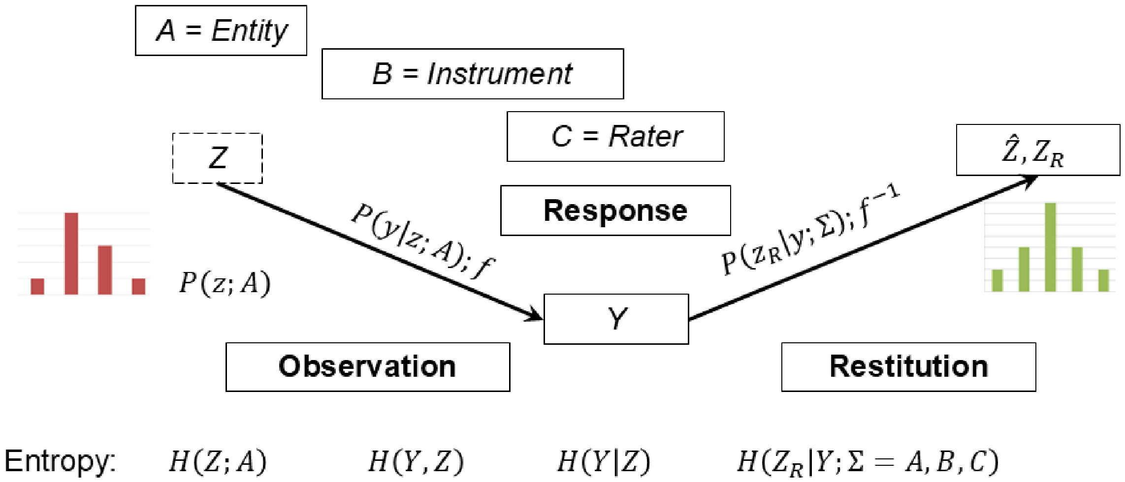
Figure 1. Probabilistic and entropy models of the measurement system and processes, inspired [2] p. 198, in part by the probabilistic model of Rossi (Figure 5.5 in [27] ). Z—measurand; Y—response; R—restitution via uncertainty model (Section 3.1); P—probability; H—entropy. The measurement process is described in terms of a metrological measurement system analysis (MSA) with measurement object (entity, A), instrument (B), and operator (C). The concept of entropy (H), evaluated (Equation (24)) for the PMF at each stage of the measurement process, is invoked to aid explanation of how information is lost, distorted or gained from observation of the measurand (Z), via response (Y) to restitution ( Z R ). The calibration function, f, relates the instrument response to the input from the measurement object.
Foundations 06 00026 g001
Figure 2. Perceived counts (‘Response location’) from a study [8] of elementary counting tasks (‘items’, j) of a set of clouds of increasing (‘stimulus’) number and counting task difficulty of dots. From Figure 2 of [8], Stanislas Dehaene et al., Log or Linear? Distinct Intuitions of the Number Scale in Western and Amazonian Indigene Cultures. Science 320, 1217–20 (2008). DOI:10.1126/science.1156540). Reprinted with permission from AAAS Licence no: 6284050178265 2026-06-08.
Foundations 06 00026 g002
Figure 3. Analytical PMFs of distributions of perceived counting errors for three counts: (1 dot, 6 dots and 8 dots) in the study [8] (data shown in Figure 2) of elementary counting tasks (‘items’, j) of sets of clouds of increasing numbers of dots and task difficulty. Lines for each count PMF assume a Gaussian distribution of counting error, p x = N ( ( μ μ 0 ) , σ 2 ), μ   = perceived count (Equation (5)); σ = 1 dot, perceived counting dispersion (Equation (6)); μ 0 = true count.
Foundations 06 00026 g003
Figure 4. PMF for simulated binomial dichotomous distribution (probability of success P s u c c e s s = 0.3 , Monte Carlo sample size 10 6 ) [37].
Foundations 06 00026 g004
Figure 5. Binomial ogive curve showing counted-fraction non-linearity at either end of the response scale (Section 4.1.2).
Foundations 06 00026 g005
Figure 6. Marginal response scores versus log-odds for the [8] dot counting data, Hartley entropy (Section 5), showing counted-fraction non-linearity (Section 4.1.2) at the lower end of the response scale. Note the opposite sign on the logit x-axis compared with the x-axis of Figure 5, which is due to the link function z = θ δ .
Foundations 06 00026 g006
Figure 7. Poisson PMFs (Equation (21), according to [57]) for three counting tasks: one dot, 6 dots and 8 dots of increasing levels of difficulty (Equation (26). Counter ability taken as the cohort mean, θ m e a n .
Foundations 06 00026 g007
Figure 9. PMFs for simulated data from psychometric analysis (Rasch Equation (17)) for a set of clouds of dots of increasing (a) (red PMF) task (‘object’) counting difficulty, δ i based on the Hartley entropy theory Equation (26) and (b) (blue PMF) counter ability, θ i , assuming a Normal distribution (Section 5.4.2) [8,9].
Foundations 06 00026 g009
Figure 10. Comparison of simulated ((Hartley entropy, Equation (26), y-axis) and calculated (x-axis) counting task difficulties from psychometric analysis (Rasch Equation (17)) of a cohort. (a) (blue) Task difficulty and (b) (orange) 10× residuals of differences between simulated and calculated difficulties. Uncertainty coverage factor, k = 2 .
Foundations 06 00026 g010
Figure 11. Comparison of simulated (Equation (27), y-axis) and calculated (x-axis) counting agent abilities from psychometric analysis (Rasch Equation (17)) of a cohort. (a) (blue) Agent ability and (b) (orange) 10× residuals of differences between simulated and calculated abilities. Uncertainty coverage factor, k = 2 .
Foundations 06 00026 g011
Figure 12. Comparison of simulated (Hartley entropy, Equation (26), y-axis) and original experimental data (x-axis) counting task difficulties from psychometric analysis (Rasch Equation (17)). Uncertainty coverage factor, k = 2 .
Foundations 06 00026 g012
Table 1. Discrete and continuous ranges versus qualitative and quantitative scales.
DiscreteContinuous
QualitativeInstrument response (Section 5.4):
P success per category/class
Clinical performance (bullet 2):
Instrument ability, θ , u( θ )
Task difficulty, δ , u( δ )
QuantitativeAnalytical counting (Section 3.3)
How many dots in object?
Counting errors
Limit of detection
Analytical measure (bullet 1):
How much of a quantity in object?
Measurement errors and uncertainties
Trueness & precision
Table 2. Empirical PMFs for three counting tasks: 1 dot, 6 dots and 8 dots.
x12345678910
P ( X = 1 ) 33.7210.772.290.370.050.00.00.00.00.0
P ( X = 6 ) 3.097.8913.4317.1517.5314.9210.896.953.952.02
P ( X = 8 ) 1.835.2710.1014.5116.6815.9713.129.426.023.46
Disclaimer/Publisher’s Note: The statements, opinions and data contained in all publications are solely those of the individual author(s) and contributor(s) and not of MDPI and/or the editor(s). MDPI and/or the editor(s) disclaim responsibility for any injury to people or property resulting from any ideas, methods, instructions or products referred to in the content.