Fisher Information in Helmholtz–Boltzmann Thermodynamics of Mechanical Systems

Abstract

In this paper, we review Helmholtz–Boltzmann thermodynamics for mechanical systems depending on parameters, and we compute the Fisher information matrix for the associated probability density. The divergence of Fisher information has been used as a signal for the existence of phase transitions in finite systems even in the absence of a thermodynamic limit. We investigate through examples if qualitative changes in the dynamic of mechanical systems described by Helmholtz–Boltzmann thermodynamic formalism can be detected using Fisher information.

1. Introduction

The first part of the paper is devoted to an introduction of Helmholtz–Boltzmann (HB) thermodynamics for mechanical systems. In [1,2], Helmholtz proved that (1) for a one-dimensional conservative mechanical system with potential energy $u(x,\mathit{\lambda })$—where $\mathit{\lambda }$ is a parameter—a probability density $p=f(e-u(x,\mathit{\lambda }\left)\right)$ can be defined on the region of configuration space corresponding to motions with energy e; moreover, (2) mechanical analogs of temperature T, pressure P, and entropy S can be introduced such that the first principle of thermodynamics in the form $TdS=de+Pd\mathit{\lambda }$ holds for these systems. In the same years, Boltzmann [3] derived the analog of the probability density p for a mechanical system of n dimensions and investigated the ergodic hypothesis for these systems. Interestingly, this picture of statistical mechanics based on a probability density defined in the configuration space preceded the Gibbs formulation of statistical mechanics [4], whose ensembles are defined on phase space. In recent times, HB thermodynamics has been investigated in a series of papers [5,6,7,8].

In the second part of this paper, we compute the Fisher Information matrix for mechanical systems described by HB thermodynamics. The Fisher information (FI) matrix [9,10], a notion originally developed in statistical estimation theory, is nowadays at the crossroads between information theory [11,12], differential geometry [13], and statistical mechanics [14]. Recently, FI has been used to detect phase transitions in machine learning [15], neural networks [16], and in quantum systems even in the absence of a thermodynamic limit [17]. For finite systems, the existence of a phase transition is related to the divergence of one or more of the FI matrix elements, or more simply, it is located in correspondence to their maxima. Within this approach, which merges statistical mechanics and information theory, divergence of FI matrix elements is used to single out order parameters and reveal phase transitions; see [18].

However, for systems described by HB thermodynamics, all the information on the dynamics is encoded in the form of the potential energy $u(x,\mathit{\lambda })$, where $x\in {\mathbb{R}}^d$ and $\mathit{\lambda }\in {\mathbb{R}}^k$, so clearly we are dealing with a finite-dimensional system that is not composed of N interacting elementary units as in statistical mechanics. Moreover, there is no clear indication for the identification of one or more parameters $\mathit{\lambda }$ as system’ volume; therefore, we cannot carry over for these systems the thermodynamic limit. We thus necessarily need to understand a possible notion of “phase transition” in a broader sense, as a qualitative change in some of the system’s features or patterns when a tunable parameter crosses a threshold, as in the bifurcation theory for dynamical systems. Essentially, with HB thermodynamics, which is a statistical theory based on a probability density $p=f(e-u(x,\mathit{\lambda }\left)\right)$, we are between the statistical mechanics and bifurcation theory approaches, and this drives the interest for these systems and shapes the tools that we are going to use.

In Section 3, we state the conditions under which the probability density $p=f(e-u(x,\mathit{\lambda }\left)\right)$ can define a statistical model and compute the related FI matrix. We examine the relationship between the elements of the FI matrix and the second-order derivatives of the free entropy for the density $p=f(e-u(x,\mathit{\lambda }\left)\right)$, which is not an exponential family, and make a comparison with the corresponding notions for the canonical density (an exponential family) used in statistical mechanics. In Section 5 we show with paradigmatic examples that the divergence in the FI elements can detect qualitative changes in the form of probability density that describe the system (which can be interpreted as a signature of phase transition in finite systems), or it can locate the transition from negative to positive specific heat. We are aware that these results are not enough to shape a general theory, but we hope that this first step may help to renew interest in the Helmholtz–Boltzmann approach to the thermodynamics of mechanical systems.

2. Helmholtz–Boltzmann Thermodynamics of Mechanical Systems

In this section, we give a short exposition of Helmholtz–Boltzmann thermodynamics. Let us consider the unidimensional motion of a point of mass m under the action of a positional force $f\left(x\right)=-u^{\prime }\left(x\right)$, where u is the potential energy. This mechanical system is conservative, and the energy integral

$${\displaystyle \frac{m}{2}}{v}^2+u\left(x\right)=e$$

defines a 1-dimensional orbit in the phase plane $(x,v)$, which can be locally described as $v(x,e)=\sqrt{{\displaystyle \frac{2}{m}}\mathit{\phi }}$ where $\mathit{\phi }=e-u$ is the kinetic energy. If the potential energy is convex, then the motion corresponding to a fixed value e of the energy is confined in the convex interval

$$H\left(e\right)=\{x\in \mathbb{R}:\mathit{\phi }=e-u>0\}=(x_1\left(e\right),x_2\left(e\right))$$

(1)

and it is periodic. Denoting with $dt=dx/v(x,e)$ the time needed to travel a space interval $dx$, the semi-period of the motion is expressed by the generalized integral

$$T\left(e\right)={\int }_{H\left(e\right)}{\displaystyle \frac{dx}{v(x,e)}}=\sqrt{{\displaystyle \frac{m}{2}}}{\int }_{H\left(e\right)}{\mathit{\phi }}^{-{\displaystyle \frac{1}{2}}}dx=\sqrt{{\displaystyle \frac{m}{2}}}Z\left(e\right).$$

(2)

We have that $v=0$ on the boundary of $H\left(e\right)$, but the generalized integral $T\left(e\right)$ is convergent if the orbit corresponding to the value of e is not a separatrix. We can thus define a probability density on $H\left(e\right)$ as (the value of m is not relevant)

$$p(x,e)={\displaystyle \frac{{\mathit{\phi }}^c(x,e)}{Z\left(e\right)}}={\displaystyle \frac{{\mathit{\phi }}^c(x,e)}{{\int }_{H\left(e\right)}{\mathit{\phi }}^c(x,e)dx}}\mathrm{w}\mathrm{h}\mathrm{e}\mathrm{r}\mathrm{e}c=-{\displaystyle \frac{1}{2}}.$$

(3)

As an example, if $u\left(x\right)=x^2$ is the elastic potential energy and $e=a^2,a>0$, we have $\mathit{\phi }=a^2-x^2$ and p is the arc-sine probability density defined in $(-a,a)$

$$p(x,a)={\displaystyle \frac{1}{Z}}{(a^2-x^2)}^{-{\displaystyle \frac{1}{2}}}={\displaystyle \frac{1}{\pi \sqrt{a^2-x^2}}}.$$

We denote with $\langle f\rangle$ the average of a function defined on $H\left(e\right)$ with respect to the probability p in (3).

The aim of Helmholtz and Boltzmann (see [5] for a historical recognition of the theory) was to provide a mechanical analogy of the first principle of thermodynamics in Gibbs form

$$TdS=de+PdV$$

where S is the entropy, T is the temperature, P is the pressure, V is the volume, and $PdV$ is the work done on the systems (hence negative).

This can be obtained by supposing that the potential energy depends on a parameter $\mathit{\lambda }$ as $u=u(x,\mathit{\lambda })$ and by defining the temperature as twice the average of $\mathit{\phi }$ (which is the kinetic energy) and the pressure as the average of ${\mathit{\phi }}_{\mathit{\lambda }}=\partial \mathit{\phi }/\partial \mathit{\lambda }$ with respect to the probability density p in (3), which now depends on $\mathit{\lambda }$:

$$T(e,\mathit{\lambda })=2\langle \mathit{\phi }\rangle ,P(e,\mathit{\lambda })=\langle {\mathit{\phi }}_{\mathit{\lambda }}\rangle .$$

(4)

The entropy S is defined as the logarithm of the area in phase space enclosed by the orbit of energy e, which gives

$$S(e,\mathit{\lambda })=ln\left(2{\int }_{H}v(x,e,\mathit{\lambda })dx\right)=ln\left(Z(e,\mathit{\lambda })\langle \mathit{\phi }\rangle \right)+const.$$

(5)

One can check that the above-defined thermodynamic analogs of $T,P,S$ for a mechanical system do satisfy the following relation, which is the mechanical equivalent of the first principle of thermodynamics

$$dS={\displaystyle \frac{\partial S}{\partial e}}de+{\displaystyle \frac{\partial S}{\partial \mathit{\lambda }}}d\mathit{\lambda }={\displaystyle \frac{1}{2\langle \mathit{\phi }\rangle }}[de+\langle {\mathit{\phi }}_{\mathit{\lambda }}\rangle d\mathit{\lambda }]={\displaystyle \frac{1}{T}}[de+Pd\mathit{\lambda }]$$

The proof is a straightforward application of the formula of derivation of an integral depending on a parameter; see [5,7].

2.1. The Multidimensional Probability Density

In [7] an extension of the above result to the case of $x\in {\mathbb{R}}^d$, $d\ge 1$ and $\mathit{\lambda }\in U\subset {\mathbb{R}}^k$ is provided (see also [8] for a different approach). For the sake of completeness and to provide a basis for further development, we give an account of it here (see Proposition 3 below). The first step is to generalize the entropy formula (5) and the probability density (3) to the d-dimensional case. To this aim, we consider a system of n particles of mass m moving in ${\mathbb{R}}^3$ referred to coordinates $x\in {\mathbb{R}}^d,d=3n$, and subject to potential energy $u(x,\mathit{\lambda })$. The total energy is ${\displaystyle \frac{m}{2}}{v}^2+u(x,\mathit{\lambda })=e$, and, analogously to what we have done before, we define

$$Q(e,\mathit{\lambda })=\{(x,v)\in {\mathbb{R}}^{2d}:{\displaystyle \frac{m}{2}}{v}^2+u(x,\mathit{\lambda })\le e\}$$

to be the portion of phase space where the energy is not greater than e. We define, as in the microcanonical approach of statistical mechanics (see [5,8] for a justification of this definition), the entropy $S(e,\mathit{\lambda })$ of the system as the logarithm of the measure of Q in phase space ${\mathbb{R}}^{2d}$, that is

$$\Sigma (e,\mathit{\lambda })={\int }_{Q(e,\mathit{\lambda })}dxdv,S(e,\mathit{\lambda })=ln\Sigma (e,\mathit{\lambda }).$$

(6)

If we set as before $\mathit{\phi }=e-u(x,\mathit{\lambda })$ and

$$H(e,\mathit{\lambda })=\{x\in {\mathbb{R}}^d:\mathit{\phi }=e-u(x,\mathit{\lambda })>0\}$$

(7)

then

$$Q(e,\mathit{\lambda })=\bigcup _{x\in H(e,\mathit{\lambda })}\{(x,v):v^2\le {\displaystyle \frac{2}{m}}\mathit{\phi }\}=\bigcup _{x\in H(e,\mathit{\lambda })}\{(x,v):v\in B_d(\sqrt{{\displaystyle \frac{2}{m}}\mathit{\phi }})\}$$

where $B_d\left(r\right)$ is the ball of radius r in ${\mathbb{R}}^d$. Let $R(x,e,\mathit{\lambda })=\sqrt{{\displaystyle \frac{2}{m}}\mathit{\phi }}$. Using Fubini’s theorem, we can factorize the above entropy integral as

$$\Sigma =e^S={\int }_{Q(e,\mathit{\lambda })}dxdv={\int }_{H(e,\mathit{\lambda })}\left({\int }_{B_d\left(R\right)}dv\right)dx$$

(8)

and the inner integral can be computed by “integrating on spheres” as

$${\int }_{B_d\left(R\right)}dv={\alpha }_d{\int }_0^R{r}^{d-1}dr={\displaystyle \frac{{\alpha }_d}{d}}{R}^d={\omega }_d{R}^d={\omega }_d{({\displaystyle \frac{2}{m}}\mathit{\phi })}^{{\displaystyle \frac{d}{2}}}$$

where ${\omega }_d$ is the measure of the unit ball in ${\mathbb{R}}^d$. Therefore, up to an unessential constant term, the entropy is

$$S(e,\mathit{\lambda })=ln{\int }_{H(e,\mathit{\lambda })}{\mathit{\phi }}^{{\displaystyle \frac{d}{2}}}dx.$$

(9)

If we define the probability density on the subset $H(e,\mathit{\lambda })\subset {\mathbb{R}}^d$ of configuration space as – see (3)–

$$p(x,e,\mathit{\lambda })={\displaystyle \frac{{\mathit{\phi }}^c}{Z(e,\mathit{\lambda })}}={\displaystyle \frac{{\mathit{\phi }}^c}{{\int }_H{\mathit{\phi }}^{c}dx}},\mathrm{w}\mathrm{h}\mathrm{e}\mathrm{r}\mathrm{e}c={\displaystyle \frac{d}{2}}-1$$

(10)

and we set in (9)

$${\int }_H{\mathit{\phi }}^{{\displaystyle \frac{d}{2}}}dx=Z{\int }_H\mathit{\phi }{\displaystyle \frac{{\mathit{\phi }}^{\frac{d}{2}-1}}{Z}}dx$$

then, the entropy integral (9) can be expressed in the same form of (5)

$$S=ln(Z\langle \mathit{\phi }\rangle ).$$

(11)

Remark 1.

We will use the above introduced probability density (10) for a generic system whose configuration space has dimension d without making reference to a point particle system. Note that for $d\ge 2$ we have $c={\displaystyle \frac{d}{2}}-1>0$; hence, a definite integral in (10) and ${\mathit{\phi }}^c$ defines a normalizable probability density.

For later use, it will be useful to express the probability density (10) in exponential form by setting

$$h=ln\mathit{\phi }(x,e,\mathit{\lambda })=ln(e-u(x,\mathit{\lambda }\left)\right),\mathrm{\Psi }=lnZ(e,\mathit{\lambda })$$

(12)

therefore, (10) can be given the form

$$p(x,e,\mathit{\lambda })={\displaystyle \frac{e^{ch}}{{\int }_H{e}^{ch}dx}}={\displaystyle \frac{e^{ch}}{Z(e,\mathit{\lambda })}}=e^{ch(x,e,\mathit{\lambda })-\mathrm{\Psi }(e,\mathit{\lambda })}$$

(13)

and the entropy in (11) becomes (here $\mathrm{\Psi }=lnZ$ is the free entropy )

$$S=ln(Z\langle \mathit{\phi }\rangle )=\mathrm{\Psi }+ln\langle \mathit{\phi }\rangle .$$

(14)

2.2. Multidimensional HB Thermodynamics

Our task now is to show that for a mechanical system described by a potential energy $u(x,\mathit{\lambda })$ with $x\in {\mathbb{R}}^d$, $\mathit{\lambda }\in U\subset {\mathbb{R}}^k$, a mechanical analog of the first principle of thermodynamics holds. In this section, we recall a number of results that will be used in the proof of the multidimensional HB thermodynamics result.

We start with recalling the Leibnitz integral rule, also called the Reynold transport theorem in continuum mechanics, which generalizes to ${\mathbb{R}}^d$ the formula of derivation for the integral depending on parameters.

Proposition 1.

Let $f=f(x,\alpha )$ be a real function depending on one or more parameters α to be integrated on a domain $D(\alpha )\subset {\mathbb{R}}^d$. Then,

$${\displaystyle \frac{\partial }{\partial \alpha }}{\int }_{D(\alpha )}fdx={\int }_{D(\alpha )}{\displaystyle \frac{\partial f}{\partial \alpha }}dx+{\int }_{\partial D}fn·vd\sigma$$

(15)

where $\partial D$ is the boundary of D, n is its outer normal unit vector, and v is the speed of the boundary. If $D=\{x\in {\mathbb{R}}^d:\mathit{\phi }(x,\alpha )\ge 0\}$, then $\partial D=\{x\in {\mathbb{R}}^d:\mathit{\phi }(x,\alpha )=0\}$, and it holds that

$$n={\displaystyle \frac{\nabla \mathit{\phi }}{|\nabla \mathit{\phi }|}},v=-{\displaystyle \frac{\frac{\partial \mathit{\phi }}{\partial \alpha }}{|\nabla \mathit{\phi }|}}n.$$

Using the above Proposition 1, we want to compute the partial derivatives of the free entropy $\mathrm{\Psi }$ in (12) with respect to $\alpha$, where $\alpha$ denotes the parameters e or $\mathit{\lambda }$. If we assume that $c>0$ so that $e^{ch}={\mathit{\phi }}^c=0$ on $\partial H$, the boundary term in (15) is vanishing, and we have (here and in the following we set $f{,}_{\alpha }=\partial f/\partial \alpha$)

$$\mathrm{\Psi }{,}_{\alpha }={\displaystyle \frac{1}{Z}}{\displaystyle \frac{\partial }{\partial \alpha }}{\int }_H{e}^{ch}dx={\displaystyle \frac{1}{Z}}{\int }_H{e}^{ch}\left(ch{,}_{\alpha }\right)dx=c\langle h{,}_{\alpha }\rangle .$$

(16)

If we introduce the log function associated to the probability density in (13)

$$l=lnp=ch-\mathrm{\Psi }$$

(17)

we get the result

$$l{,}_{\alpha }=ch{,}_{\alpha }-\mathrm{\Psi }{,}_{\alpha }=c(h{,}_{\alpha }-\langle h{,}_{\alpha }\rangle )={\displaystyle \frac{p{,}_{\alpha }}{p}}$$

(18)

and we can prove the following useful formula:

Proposition 2.

Let $f=f(x,\alpha )$ be a real function such that $fp=0$ on $\partial H$. Then, we have that

$$\begin{array}{ccc}\hfill \langle f\rangle {,}_{\alpha }& =& {\displaystyle \frac{\partial }{\partial \alpha }}{\int }_{H}fpdx={\int }_H\left(fp\right){,}_{\alpha }dx={\int }_H(f{,}_{\alpha }p+fp{,}_{\alpha })dx\hfill \\ & =& \langle f{,}_{\alpha }\rangle +c{\int }_{H}fp(h{,}_{\alpha }-\langle h{,}_{\alpha }\rangle )dx\hfill \\ & =& \langle f{,}_{\alpha }\rangle +c(\langle fh{,}_{\alpha }\rangle -\langle f\rangle \langle h{,}_{\alpha }\rangle )\hfill \\ & =& \langle f{,}_{\alpha }\rangle +ccov(f,h{,}_{\alpha })=\langle f{,}_{\alpha }\rangle +ccov(f,{\displaystyle \frac{\mathit{\phi }{,}_{\alpha }}{\mathit{\phi }}}).\hfill \end{array}$$

As a straightforward application of Proposition 2 for $f=\mathit{\phi }$, we can compute (here $h{,}_{\alpha }={\displaystyle \frac{\mathit{\phi }{,}_{\alpha }}{\mathit{\phi }}}$)

$$\langle \mathit{\phi }\rangle {,}_{\alpha }=\langle \mathit{\phi }{,}_{\alpha }\rangle +c\left(\langle \mathit{\phi }h{,}_{\alpha }\rangle -\langle \mathit{\phi }\rangle \langle h{,}_{\alpha }\rangle \right)=(1+c)\langle \mathit{\phi }{,}_{\alpha }\rangle -c\langle \mathit{\phi }\rangle \langle h{,}_{\alpha }\rangle .$$

(19)

Now all the elements to prove the multidimensional version of HB thermodynamics have been introduced.

Proposition 3.

Let the entropy function for a mechanical system with potential energy $u(x,\mathit{\lambda })$ be

$$S(e,\mathit{\lambda })=ln{\int }_{H(e,\mathit{\lambda })}{\mathit{\phi }}^{{\displaystyle \frac{d}{2}}}dx=lnZ+ln\langle \mathit{\phi }\rangle =\mathrm{\Psi }+ln\langle \mathit{\phi }\rangle$$

and define the temperature $T(e,\mathit{\lambda })$ and the i-type pressure $P_i(e,\mathit{\lambda })$ as

$$T={\displaystyle \frac{\langle \mathit{\phi }\rangle }{1+c}}={\displaystyle \frac{2}{d}}\langle \mathit{\phi }\rangle ,P_i=\langle {\mathit{\phi }}_{,{\mathit{\lambda }}_i}\rangle .$$

(20)

Then it holds that

$$dS={\displaystyle \frac{1}{T}}[de+\sum _i{P}_{i}d{\mathit{\lambda }}_i]$$

Proof. 

Let $\alpha =e$ or $\alpha ={\mathit{\lambda }}_i$, $i=1,\dots ,k$. We have from (16) and (19) that

$$S_{,\alpha }={\mathrm{\Psi }}_{,\alpha }+{(ln\langle \mathit{\phi }\rangle )}_{,\alpha }=c\langle h_{,\alpha }\rangle +{\displaystyle \frac{1}{\langle \mathit{\phi }\rangle }}[(1+c)\langle {\mathit{\phi }}_{,\alpha }\rangle -c\langle \mathit{\phi }\rangle \langle h_{,\alpha }\rangle ]={\displaystyle \frac{1+c}{\langle \mathit{\phi }\rangle }}\langle {\mathit{\phi }}_{,\alpha }\rangle$$

and, since ${\mathit{\phi }}_{,e}=1$, we derive that for $S(e,\mathit{\lambda })$

$$dS={\displaystyle \frac{\partial S}{\partial e}}de+\sum _{i=1}^k{\displaystyle \frac{\partial S}{\partial {\mathit{\lambda }}_i}}d{\mathit{\lambda }}_i={\displaystyle \frac{1+c}{\langle \mathit{\phi }\rangle }}[de+\sum _{i=1}^k\langle \mathit{\phi }{,}_{{\mathit{\lambda }}_i}\rangle d{\mathit{\lambda }}_i]$$

$$={\displaystyle \frac{1}{T}}[de+\sum _i{P}_{i}d{\mathit{\lambda }}_i]$$

□

From the above result, temperature and pressure can be computed using the relations

$$T^{-1}={\displaystyle \frac{\partial S}{\partial e}},{\displaystyle \frac{P_i}{T}}={\displaystyle \frac{\partial S}{\partial {\mathit{\lambda }}_i}}.$$

(21)

2.3. Relation with Microcanonical Entropy

In this section, we compute the microcanonical entropy, the related temperature, and the specific heat to be compared with the same objects defined in HB thermodynamics. In HB thermodynamics, the entropy is the volume entropy defined as $S=ln\Sigma$, as in (6). To define the entropy of the microcanonical ensemble, we introduce the so-called density of states $g(e,\mathit{\lambda })$ and the microcanonical entropy $S_{\mu }$

$$g(e,\mathit{\lambda })={\displaystyle \frac{\partial \Sigma (e,\mathit{\lambda })}{\partial e}},S_{\mu }(e,\mathit{\lambda })=lng(e,\mathit{\lambda }).$$

Since from (9)

$$\Sigma (e,\mathit{\lambda })={\omega }_d{\int }_H{\mathit{\phi }}^{c+1}(x,e,\mathit{\lambda })dx$$

we have

$$g(e,\mathit{\lambda })={\displaystyle \frac{\partial \Sigma (e,\mathit{\lambda })}{\partial e}}=(c+1){\omega }_d{\int }_H{\mathit{\phi }}^{c}dx=(c+1){\omega }_{d}Z(e,\mathit{\lambda })$$

therefore, up to constant terms, the microcanonical entropy $S_{\mu }$ is

$$S_{\mu }(e,\mathit{\lambda })=lng(e,\mathit{\lambda })=lnZ(e,\mathit{\lambda })=\mathrm{\Psi }(e,\mathit{\lambda })$$

(22)

and we have from (14) the relation between HB and microcanonical entropy

$$S=S_{\mu }+ln\langle \mathit{\phi }\rangle .$$

For most thermodynamic systems, the two definitions of entropy are equivalent in the limit of $n\to \infty$, where n is the number of particles of the system, see e.g., [19]. If we define the microcanonical temperature as $T_{\mu }^{-1}=\partial S_{\mu }/\partial e$ we have, from (22) and (16)

$${\displaystyle \frac{1}{T_{\mu }}}={\displaystyle \frac{\partial S_{\mu }}{\partial e}}=\mathrm{\Psi }{,}_e=c\langle {\displaystyle \frac{1}{\mathit{\phi }}}\rangle$$

(23)

which is different from the definition of temperature in HB thermodynamics, $T=2\langle \mathit{\phi }\rangle /d$, see (20). So the two ensembles, for finite number of degree of freedom systems, are non-equivalent.

We now compute the specific heat in the HB and microcanonical cases. Note that since the temperature in HB thermodynamics is defined as the average value of the kinetic energy, $c_v$ is a dimensionless quantity. We define

$${\displaystyle \frac{1}{c_v}}={\displaystyle \frac{dT}{de}}={\displaystyle \frac{2}{d}}\langle \mathit{\phi }\rangle {,}_e$$

and using again Proposition 2 we get

$${\displaystyle \frac{1}{c_v}}={\displaystyle \frac{2}{d}}[\langle \mathit{\phi }{,}_e\rangle +ccov(\mathit{\phi },h{,}_e)]={\displaystyle \frac{2}{d}}[1+c-c\langle \mathit{\phi }\rangle \langle {\displaystyle \frac{1}{\mathit{\phi }}}\rangle ]=1-{\displaystyle \frac{T}{T_{\mu }}}$$

(24)

so the specific heat $c_v$ diverges when $T=T_{\mu }$. Using the microcanonical temperature (23) we have

$${\displaystyle \frac{d}{de}}\left(T_{\mu }^{-1}\right)=-{\displaystyle \frac{1}{T_{\mu }^2}}{\displaystyle \frac{d{T}_{\mu }}{de}}=-{\displaystyle \frac{1}{T_{\mu }^2}}{\displaystyle \frac{1}{c_{v\mu }}}=c\langle {\displaystyle \frac{1}{\mathit{\phi }}}\rangle {,}_e=-c\langle {\displaystyle \frac{1}{{\mathit{\phi }}^2}}\rangle +c^{2}var({\displaystyle \frac{1}{\mathit{\phi }}})$$

where in the last equality above we have used Proposition 2. Therefore

$${\displaystyle \frac{1}{c_{v\mu }}}=T_{\mu }^2\left[c\langle {\displaystyle \frac{1}{{\mathit{\phi }}^2}}\rangle -c^{2}var({\displaystyle \frac{1}{\mathit{\phi }}})\right]$$

Note that, unlike what happens with the canonical ensemble, where the specific heat is necessarily positive (see (36) below), in the HB and microcanonical case the specific heat can be negative.

3. Statistical Models and Fisher Matrix

The notion of Fisher information matrix [9,10] is fundamental to describing the geometry of statistical models. We start by recalling the definition of a regular statistical model; see [12,13]. Let $p_{\theta }\left(x\right)$ be a probability density defined on state space X depending on finitely many parameters $\theta \in \mathcal{Z}\subset {\mathbb{R}}^d$. We introduce the set

$$S=\{p_{\theta }=p(x,\theta ):\theta \in \mathcal{Z}\}\subset L^1\left(X\right)$$

(25)

Definition 1.

$S$ is a regular statistical model if the following conditions (1) and (2) hold:

(1) 

(injectivity) the map $f:\mathcal{Z}\to S$, $\theta \mapsto f\left(\theta \right)=p_{\theta }$ is one to one and

(2) 

(regularity) the d functions defined on X

$$p_i(x,\theta )={\displaystyle \frac{\partial p}{\partial {\theta }_i}}(x,\theta ),i=1,\dots ,d$$

are linearly independent as functions on X for every $\theta \in \mathcal{Z}$.

The inverse $\mathit{\phi }:S\to \mathcal{Z}$, $\mathit{\phi }\left(p_{\theta }\right)=\theta$ of the map f, which exists by (1), defines a global coordinate system for $S$. It is convenient to introduce the log-likelihood $l=lnp$ and the score basis $l_i=\partial l/\partial {\theta }_i$. Note that since $l_i=(1/p)p_i$, the function $p_i$ and $l_i$ are proportional; therefore, the regularity condition (2) above holds if and only if the elements of the score basis are independent functions over X. The elements of the Fisher matrix are defined as follows:

$$g_{ij}\left(\theta \right)=\langle l_i{l}_j\rangle ={\int }_X{\displaystyle \frac{\partial l}{\partial {\theta }_i}}{\displaystyle \frac{\partial l}{\partial {\theta }_j}}p(x,\theta )dx.$$

(26)

The Fisher matrix is symmetric and positive definite; therefore, it defines a Riemannian metric on $\mathcal{Z}$ (see [13], p. 24). In fact, we have (sum over repeated indices is understood)

$$g_{ij}{v}_i{v}_j=\langle l_i{l}_j{v}_i{v}_j\rangle =\langle {\left(l_i{v}_i\right)}^2\rangle =0\iff l_i{v}_i=0\iff v_i=0\forall i$$

(27)

since the score vectors $l_i$ are linearly independent over X. Note also that g is invariant with respect to change in coordinates in the state space X, and covariant (as an order 2 tensor) with respect to change in coordinates in the parameter space [13].

Statistical Models in HB Thermodynamics

In this section we consider the HB-type probability density introduced in (13) and we compute the related Fisher matrix. We define the parameters $\theta \in \mathcal{Z}\subset {\mathbb{R}}^{1+k}$ where

$${\theta }_0=e,{\theta }_i={\mathit{\lambda }}_i,i=1,\dots k.$$

(28)

and the probability density –see (13)–

$$p(x,\theta )=e^{ch\left(\theta \right)-\mathrm{\Psi }\left(\theta \right)}={\displaystyle \frac{{\mathit{\phi }}^c(x,\theta )}{{\int }_{H\left(\theta \right)}{\mathit{\phi }}^c(x,\theta )dx}},c={\displaystyle \frac{d}{2}}-1$$

(29)

defined on the set

$$H\left(\theta \right)=\{x\in {\mathbb{R}}^d:\mathit{\phi }={\theta }_0-u(x,\theta )>0\}.$$

Unlike the theory exposed above in Section 3, the probability densities $p_{\theta },\theta \in \mathcal{Z}$ in (29) are not defined in the same sample space X. To embed this case in the previously exposed theory, we need to embed every probability density in the same space ${\mathbb{R}}^d$ by setting

$$\tilde{p}(x,\theta )=\left\{\begin{array}{cc}p(x,\theta )\hfill & \mathrm{if}x\in H\left(\theta \right)\hfill \\ 0\hfill & \mathrm{if}x\notin H\left(\theta \right)\hfill \end{array}\right.$$

(30)

In the following we will spare the tilde symbol in $\tilde{p}(x,\theta )$. We suppose that conditions (1) and (2) do hold for $p(x,\theta )$. If we compute the score basis we have from (17) and (18),

$$l_i={\displaystyle \frac{\partial l}{\partial {\theta }_i}}=ch{,}_i-\mathrm{\Psi }{,}_i=c(h{,}_i-\langle h{,}_i\rangle )=c\left({\displaystyle \frac{\mathit{\phi }{,}_i}{\mathit{\phi }}}-\langle {\displaystyle \frac{\mathit{\phi }{,}_i}{\mathit{\phi }}}\rangle \right),i=0,\dots k$$

and the elements of the Fisher matrix (26) are

$$g_{ij}\left(\theta \right)=\langle l_i{l}_j\rangle =c^2〈(h{,}_i-\langle h{,}_i\rangle )(h{,}_j-\langle h{,}_j\rangle )〉=c^{2}cov(h{,}_i,h{,}_j).$$

(31)

Another useful expression for the elements of the Fisher matrix can be deduced from Proposition 2: we have from (16) that $\mathrm{\Psi }{,}_i=c\langle h{,}_i\rangle$; hence,

$$\mathrm{\Psi }{,}_{ij}=c{\langle h{,}_i\rangle }_{,j}=c[\langle h{,}_{ij}\rangle +ccov(h{,}_i,h{,}_j)]=c\langle h{,}_{ij}\rangle +g_{ij}$$

therefore

$$g_{ij}=\mathrm{\Psi }{,}_{ij}-c\langle h{,}_{ij}\rangle .$$

(32)

Note that the Fisher matrix does not coincide with second-order derivatives of the free entropy function $\mathrm{\Psi }$. However, the above formula coincides with the one obtained for the Fisher matrix for generalized exponential families [20,21]. Below we give detailed formulas for the elements of the Fisher matrix associated with HB thermodynamics. From (28) and (12) we have

$$h{,}_0={\displaystyle \frac{\mathit{\phi }{,}_0}{\mathit{\phi }}}={\displaystyle \frac{1}{\mathit{\phi }}},h{,}_i={\displaystyle \frac{\mathit{\phi }{,}_i}{\mathit{\phi }}}=-{\displaystyle \frac{u{,}_i}{\mathit{\phi }}}$$

so that

$$g_{00}\left(\theta \right)=c^{2}cov(h{,}_0,h{,}_0)=c^2\left[\langle {\displaystyle \frac{1}{{\mathit{\phi }}^2}}\rangle -{\langle {\displaystyle \frac{1}{\mathit{\phi }}}\rangle }^2\right]=c^{2}var({\displaystyle \frac{1}{\mathit{\phi }}})$$

(33)

and

$$g_{0i}\left(\theta \right)=c^{2}cov(h{,}_0,h{,}_i)=c^2\left[\langle {\displaystyle \frac{-u{,}_i}{{\mathit{\phi }}^2}}\rangle -\langle {\displaystyle \frac{1}{\mathit{\phi }}}\rangle \langle {\displaystyle \frac{-u{,}_i}{\mathit{\phi }}}\rangle \right]$$

and

$$g_{ij}\left(\theta \right)=c^{2}cov(h{,}_i,h{,}_j)=c^2\left[\langle {\displaystyle \frac{u{,}_{i}u{,}_j}{{\mathit{\phi }}^2}}\rangle -\langle {\displaystyle \frac{u{,}_i}{\mathit{\phi }}}\rangle \langle {\displaystyle \frac{u{,}_j}{\mathit{\phi }}}\rangle \right]$$

More in detail, the explicit expression of the Fisher matrix elements involves the computation of integrals of the type

$$\langle {\displaystyle \frac{1}{{\mathit{\phi }}^2}}\rangle ={\int }_{H\left(\theta \right)}p(x,\theta ){\displaystyle \frac{1}{{\mathit{\phi }}^2}}dx={\displaystyle \frac{1}{Z\left(\theta \right)}}{\int }_{H\left(\theta \right)}{\mathit{\phi }}^{c-2}dx$$

(34)

where $f={\mathit{\phi }}^{c-2}$ satisfies the condition $f=0$ on $\partial H$ if $c-2=(d-6)/2\ge 0$.

4. Fisher Matrix for Canonical Ensemble

In this section, we recall a well-known relation between the Fisher matrix and second-order derivatives of the canonical free entropy function. In statistical mechanics, a system of N microscopic units can be described by the Boltzmann–Gibbs (BG) or canonical probability density

$$p\left(x\right)=e^{-\beta H\left(x\right)-\mathrm{\Psi }\left(\beta \right)},\mathrm{\Psi }\left(\beta \right)=lnZ\left(\beta \right)=\int e^{-\beta H\left(x\right)}dx$$

(35)

where $H\left(x\right)$ is the Hamiltonian and the integral (or sum) is extended over the set of system states x. The inverse temperature $\beta =1/kT$ can be related to the system energy $e=\langle H\rangle$ by inverting the equation $e\left(\beta \right)=-\mathrm{\Psi }{,}_{\beta }\left(\beta \right)$ so that $\beta =\beta \left(e\right)$. As a consequence

$${\displaystyle \frac{{\partial }^2\mathrm{\Psi }}{\partial {\beta }^2}}=var(H)=-{\displaystyle \frac{de}{d\beta }}=-{({\displaystyle \frac{d\beta }{de}})}^{-1}={({\displaystyle \frac{1}{k{T}^2}}{\displaystyle \frac{dT}{de}})}^{-1}=k{T}^2{c}_v>0.$$

(36)

Second-order phase transitions are characterized by discontinuities in the function $\mathrm{\Psi }{,}_{\beta \beta }$. $\mathrm{\Psi }$ is an analytic function for finite systems, but in the thermodynamic limit, $f={lim}_N{\displaystyle \frac{1}{N}}\mathrm{\Psi }$ can develop discontinuities. If now we consider the log-likelihood of the canonical probability density $l=lnp=-\beta H-\mathrm{\Psi }$ in (35), we have

$$l_{\beta }={\displaystyle \frac{\partial l}{\partial \beta }}=-H-\mathrm{\Psi }{,}_{\beta }=-H+\langle H\rangle$$

and the Fisher information of the canonical density (35) is

$$g_{\beta \beta }=\langle l_{\beta }^2\rangle =var\left(H\right)={\displaystyle \frac{{\partial }^2\mathrm{\Psi }}{\partial {\beta }^2}}.$$

(37)

So, from (36) and (37), we get the important result that for an exponential family density, the Fisher matrix coincides with the second-order derivatives of the free entropy and that the diagonal elements of the Fisher matrix diverge at the phase transition when $c_v$ tends to infinity.

If the system Hamiltonian is in the form $\theta ·X={\sum }_{i=1}^k{\theta }_i{X}_i$ the above relations are generalized as

$$\langle X_i\rangle =-{\displaystyle \frac{\partial \mathrm{\Psi }}{\partial {\theta }_i}},g_{ij}=-{\displaystyle \frac{\partial \langle X_i\rangle }{\partial {\theta }_j}}={\displaystyle \frac{{\partial }^2\mathrm{\Psi }}{\partial {\theta }_i{\theta }_j}}=cov(X_i,X_j).$$

(38)

In [18] the above argument is reversed, and the claim is that the divergence of the diagonal elements of the Fisher matrix is a signature of a phase transition even if the underlying probability density is not the canonical one. The same argument is developed in [15] in relation to the study of phase transitions using machine learning methods. In both cases the phase transitions are located in parameter space where the diagonal elements of the Fisher matrix diverge. To conclude, we recall that phase transitions have been defined for finite systems or for systems with long-range interactions using the non-convexity of the entropy function or the non-equivalence of canonical and microcanonical ensembles (see [22,23]).

5. Fisher Matrix in HB Thermodynamics. Examples

The HB thermodynamic formalism allows us to define a probability density see (10), which is related to the microcanonical one, but it is “projected” on the configuration space. Instead of prescribing the interaction between the elementary units of the system, all the information about the system is encoded in its potential energy $u(x,\theta )$, depending on multiple parameters and the energy ${\theta }_0$. So we are using a formalism, which loosely speaking is in between statistical mechanics and catastrophe theory, and a probability density, which is not an exponential family. Nevertheless, we still have, see (16) and (32), that for multidimensional HB thermodynamics —compare with (38)

$$\mathrm{\Psi }{,}_{\alpha }=c\langle h{,}_{\alpha }\rangle ,g_{ij}\left(\theta \right)=c^{2}cov(h{,}_i,h{,}_j)={\displaystyle \frac{{\partial }^2\mathrm{\Psi }}{\partial {\theta }_i\partial {\theta }_j}}-c\langle h{,}_{ij}\rangle .$$

We want to investigate whether the divergence of elements of the Fisher matrix for particular values of parameters $\theta$ can detect qualitative changes in the dynamics in mechanical systems described by potential energy $u(x,\theta )$.

In the following, we consider some examples where the potential energy $u(x,\theta )$, $x\in {\mathbb{R}}^d$, is described by a radial function such that $u(x,\mathit{\lambda })=w\left(\right|x|,\mathit{\lambda })$. This allows us to investigate our claim while keeping the computations at a tractable level. Note that, apart from the elastic chain, all the examples below define a statistical model, as it is easy to check using Definition 1.

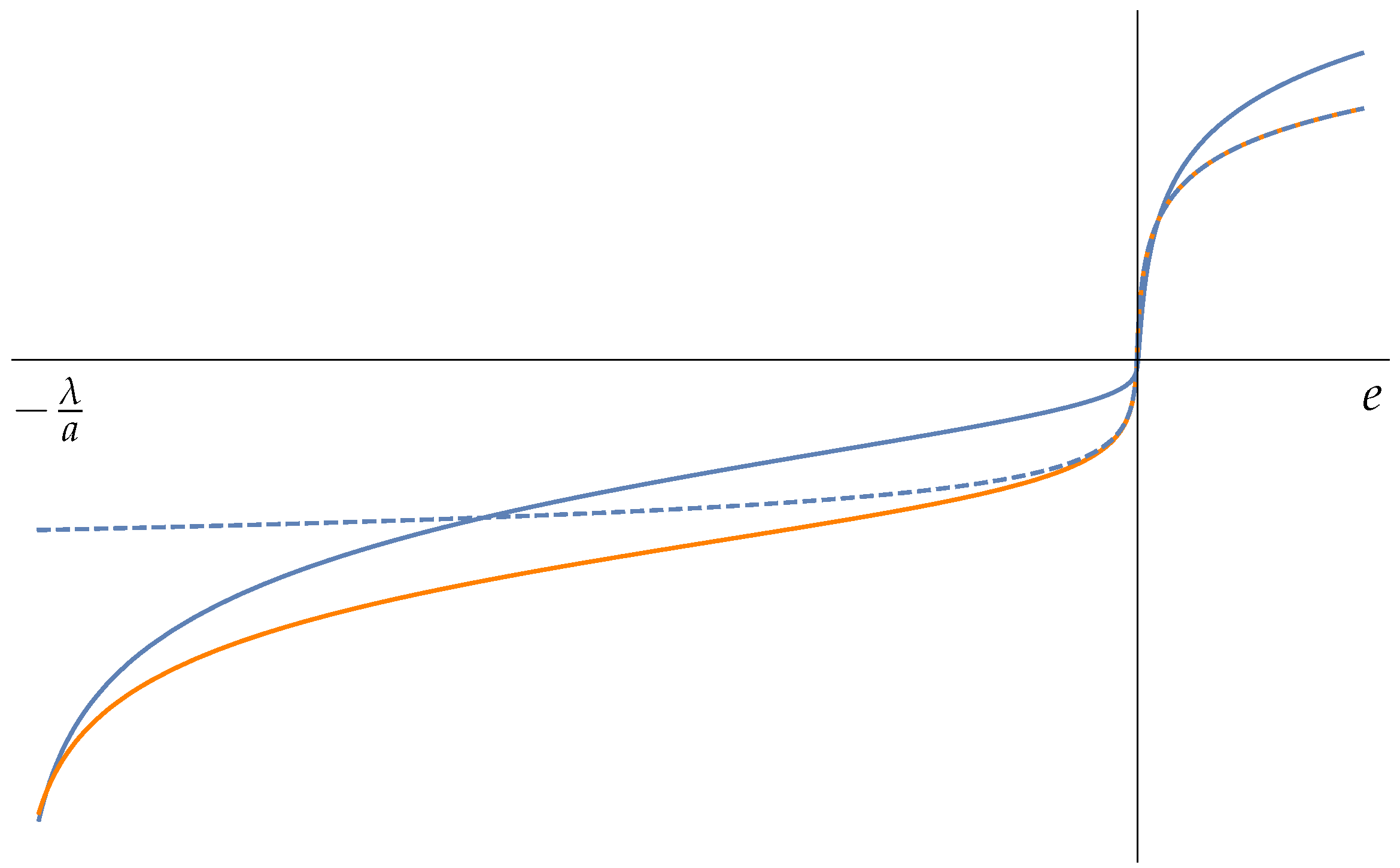
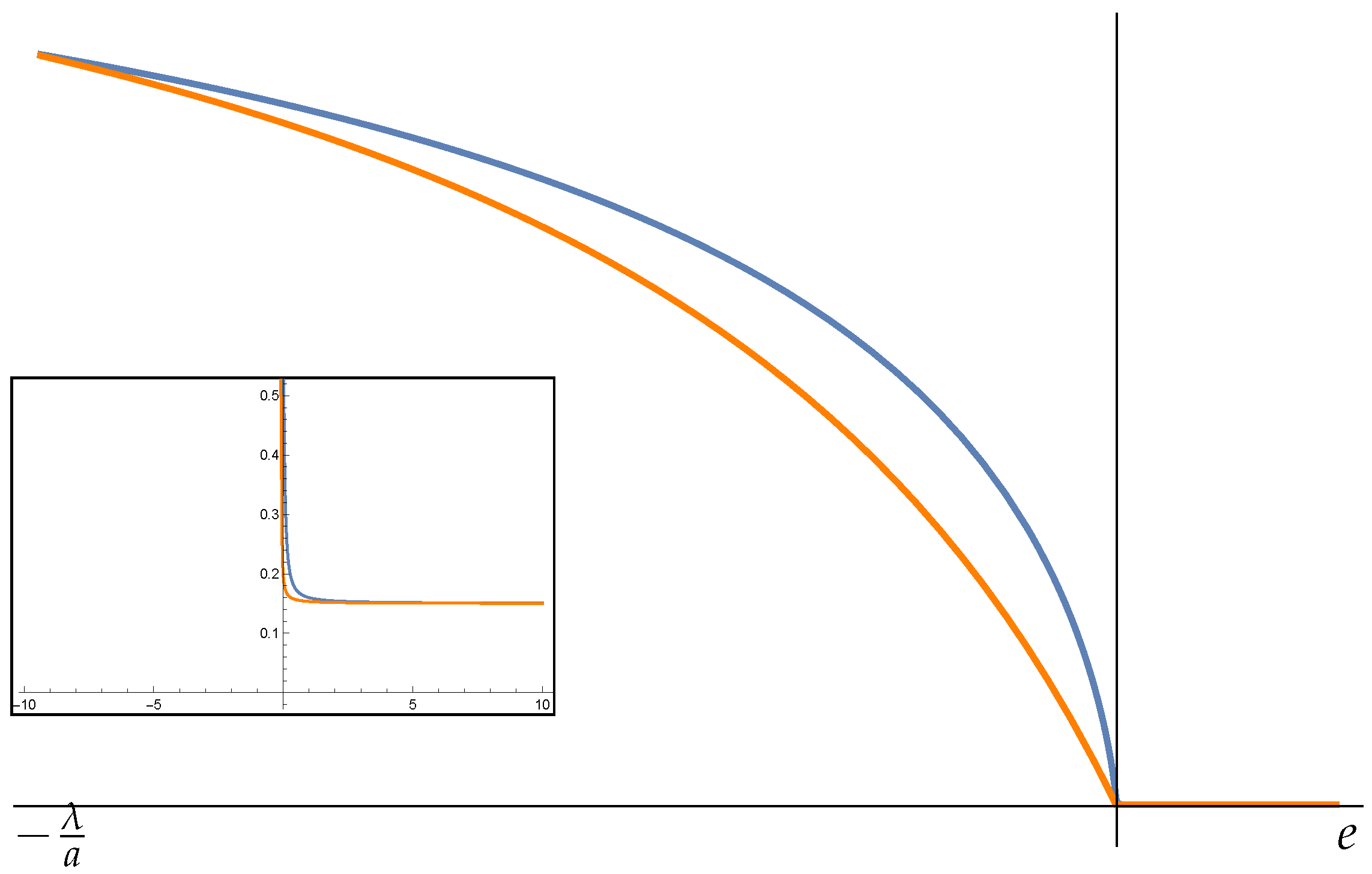
5.1. Harmonic Potential Energy

Let us consider the simplest potential energy with no external parameters $w\left(\right|x\left|\right)=x·x=x^2$ with $x\in {\mathbb{R}}^d$. This energy represents d independent one-dimensional harmonic oscillators. Then, $\mathit{\phi }=e-x^2$ and $H\left(e\right)=B_d\left(\sqrt{e}\right)$, the ball of radius $\sqrt{e}$ in ${\mathbb{R}}^d$. Let us compute

$$Z\left(e\right)={\int }_{H\left(e\right)}{\mathit{\phi }}^c(x,e)dx={\alpha }_d{\int }_0^{\sqrt{e}}{(e-r^2)}^c{r}^{d-1}dr,$$

$$\Sigma \left(e\right)={\int }_{H\left(e\right)}{\mathit{\phi }}^{c+1}(x,e)dx={\alpha }_d{\int }_0^{\sqrt{e}}{(e-r^2)}^{c+1}{r}^{d-1}dr$$

so that

$$Z\left(e\right)={\displaystyle \frac{\sqrt{\pi }\mathrm{\Gamma }\left(\frac{d}{2}\right)}{2^d\mathrm{\Gamma }\left(\frac{d+1}{2}\right)}}{e}^{d-1},\Sigma \left(e\right)={\displaystyle \frac{\sqrt{\pi }\mathrm{\Gamma }\left(\frac{d}{2}\right)}{2^{d+1}\mathrm{\Gamma }\left(\frac{d+1}{2}\right)}}{e}^d$$

where $\mathrm{\Gamma }$ is the Gamma function and the entropy function are

$$S\left(e\right)=ln\Sigma =dlne+ln[{\displaystyle \frac{\sqrt{\pi }\mathrm{\Gamma }(d/2)}{2^{d+1}\mathrm{\Gamma }\left(\frac{d+1}{2}\right)}}],S_{\mu }=lnZ=(d-1)lne+ln[{\displaystyle \frac{\sqrt{\pi }\mathrm{\Gamma }(d/2)}{2^d\mathrm{\Gamma }\left(\frac{d+1}{2}\right)}}].$$

By direct computation we get the temperature

$$T={({\displaystyle \frac{\partial S}{\partial e}})}^{-1}={\displaystyle \frac{e}{d}}={\displaystyle \frac{2}{d}}\langle \mathit{\phi }\rangle ,T_{\mu }={({\displaystyle \frac{\partial S_{\mu }}{\partial e}})}^{-1}={\displaystyle \frac{e}{d-1}}={\displaystyle \frac{1}{c\langle \frac{1}{\mathit{\phi }}\rangle }}$$

and the specific heat can be computed from $c_v^{-1}=dT/de$ giving

$$c_v=d,c_{v\mu }=d-1$$

a result that holds also in Boltzmann–Gibbs statistical mechanics (see [19]). The one dimensional Fisher matrix, also called Fisher information, is, see (33)

$$g_{00}=c^{2}var({\displaystyle \frac{1}{\mathit{\phi }}})=c^2\left[\langle {\displaystyle \frac{1}{{\mathit{\phi }}^2}}\rangle -{\langle {\displaystyle \frac{1}{\mathit{\phi }}}\rangle }^2\right]=c^2\langle {\displaystyle \frac{1}{{\mathit{\phi }}^2}}\rangle -{\displaystyle \frac{1}{T_{\mu }^2}}$$

(39)

where the probability density (29) is $p(x,e)={\mathit{\phi }}^c/Z\left(e\right)$ and

$$\langle {\displaystyle \frac{1}{{\mathit{\phi }}^2}}\rangle ={\displaystyle \frac{1}{Z\left(e\right)}}{\int }_{H\left(e\right)}{\mathit{\phi }}^{c-2}dx={\displaystyle \frac{4(d-1)}{(d-4)e^2}},$$

thereby obtaining (note that the average value exists for $d>4$)

$$g_{00}\left(e\right)={\displaystyle \frac{d(d-1)}{(d-4)}}{\displaystyle \frac{1}{e^2}}={\displaystyle \frac{1}{(d-4)}}{\displaystyle \frac{1}{T{T}_{\mu }}}$$

We see that $g_{00}\left(e\right)$ diverges for $e\to 0^{+}$, that is, when the system energy e tends to the minimum of the potential energy u.

This quadratic potential energy system is the prototype of the description of a mechanical system in the vicinity of a minimum of the potential energy. By a translation of the reference frame, we can suppose that the minimum is in $x=0$ and that $u\left(0\right)=0$ so that, using a Taylor expansion, we have

$$u\left(x\right)=u\left(0\right)+u^{\prime }\left(0\right)·x+{\displaystyle \frac{1}{2}}{u}^{″}\left(0\right)x·x+\mathcal{O}\left(3\right)$$

and

$$min(\mathit{\lambda })x^2\le u^{″}\left(0\right)x·x\le max(\mathit{\lambda })x^2$$

where $min(\mathit{\lambda })$ and $max(\mathit{\lambda })$ are the smallest and greatest (real) eigenvalues of the symmetric matrix $u^{″}\left(0\right)$. So we can conclude that the Fisher information diverges when the energy e approaches the minimum of the potential energy from above. This can be interpreted by recalling that the Fisher information measures the change in the “shape” of the probability distribution $p(x,e)$ with respect to a change in the parameter e; when the energy becomes equal to the minimum of the potential energy, the probability density becomes a Dirac delta concentrated at the minimum $x=0$. We can say that the divergence of the Fisher information $g_{00}$ at $e=0$ corresponds to the qualitative “phase transition” between a point orbit and a set of d closed orbits for the d oscillators when $e>0$.

5.2. The Elastic Chain

The following example shows that for an n-dimensional mechanical system with convex potential energy, HB thermodynamics gives a sound description of the system’s behavior (see also [7]).

Let us consider a chain of $n+1$ point particles of mass m linked by linearly elastic springs of rest length $\mathit{\lambda }$ and constrained to move on the real axis. Suppose that particle 0 is fixed in the origin and that the coordinate of the n-th particle is $\mathit{\lambda }n$ so that the length $\mathit{\lambda }n$ of the chain is a controlled parameter $\mathit{\lambda }$ corresponding to the equilibrium length of the n springs. Let the elongation of the spring $i=1,\dots n$ be written as $u_i=\mathit{\lambda }+x_i$. The length constraint is

$$\sum _{i=1}^n{u}_i=\sum _{i=1}^n(\mathit{\lambda }+x_i)=n\mathit{\lambda },\mathrm{t}\mathrm{h}\mathrm{a}\mathrm{t} \mathrm{i}\mathrm{s}\sum _{i=1}^n{x}_i=0.$$

Due to the length constraint, the chain potential energy of the resulting $n-1$ dimensional system can be written as

$$u\left(x\right)=u(x_1,\dots ,x_n)={\displaystyle \frac{h}{2}}\sum _{i=1}^n{(x_i+\mathit{\lambda })}^2={\displaystyle \frac{h}{2}}(x^2+n{\mathit{\lambda }}^2),\sum _{i=1}^n{x}_i=0$$

where $x^2={\sum }_{i=1}^n{x}_i^2$. Therefore the region $H(e,\mathit{\lambda })$ is

$$H(e,\mathit{\lambda })=\{x\in {\mathbb{R}}^n\mathit{\phi }=e-u\left(x\right)=e-{\displaystyle \frac{h}{2}}(x^2+n{\mathit{\lambda }}^2)>0,\sum _{i=1}^n{x}_i=0\}$$

i.e.,

$$H(e,\mathit{\lambda })=\{x\in {\mathbb{R}}^n:x^2<{\displaystyle \frac{2e}{h}}-n{\mathit{\lambda }}^2,\sum _{i=1}^n{x}_i=0\}=B_n\left(a\right)\cap L=B_{n-1}\left(a\right)$$

where $B_n\left(a\right)$ is the ball in ${\mathbb{R}}^n$ of radius a,

$$a^2(e,\mathit{\lambda })={\displaystyle \frac{2e}{h}}-n{\mathit{\lambda }}^2$$

and L is the $n-1$ dimensional hyperplane ${\sum }_{i=1}^n{x}_i=0$. We compute the entropy $S=ln\Sigma$ by setting

$$\mathit{\phi }=e-u={\displaystyle \frac{h}{2}}(a^2-x^2)$$

and (here $c={\displaystyle \frac{d}{2}}-1={\displaystyle \frac{n-3}{2}}$ )

$$S=ln\Sigma =ln{\int }_{H(e,\mathit{\lambda })}{\mathit{\phi }}^{c+1}dx=ln{\int }_{B_{n-1}\left(a\right)}{\displaystyle \frac{h}{2}}{(a^2-x^2)}^{c+1}dx.$$

By standard computation on radial function we get

$$S(e,\mathit{\lambda })=(n-1)ln{a}^2(e,\mathit{\lambda })+\mathrm{c}\mathrm{o}\mathrm{s}\mathrm{t}\left(n\right)=(n-1)ln(e-n{\displaystyle \frac{h}{2}}{\mathit{\lambda }}^2)+\mathrm{c}\mathrm{o}\mathrm{s}\mathrm{t}\left(n\right)$$

Let us compute the temperature of this elongated chain using

$$T={({\displaystyle \frac{\partial S}{\partial e}})}^{-1}={\displaystyle \frac{a^2}{n-1}}={\displaystyle \frac{1}{n-1}}(e-n{\displaystyle \frac{h}{2}}{\mathit{\lambda }}^2)$$

which coincides with the kinetic energy $e-u(\mathit{\lambda })$ per degree of freedom. Let us compute the pressure P corresponding to the controlled parameter $\mathit{\lambda }$ which is the elongation on the elastic chain using ${\left(\mathrm{20}\right)}_2$. We have

$$P=\langle {\displaystyle \frac{\partial \mathit{\phi }}{\partial \mathit{\lambda }}}\rangle =\langle -nh\mathit{\lambda }\rangle =-nh\mathit{\lambda }$$

which corresponds to our physical intuition of the reaction force exerted by the chain on its controlled end. The specific heat $c_v=de/dT$ is

$${\displaystyle \frac{1}{c_v}}={\displaystyle \frac{dT}{de}}={\displaystyle \frac{1}{n-1}}={\displaystyle \frac{1}{d}}.$$

Remark 2.

Note that the elastic chain model fails to define a statistical model because conditions (1) and (2) in Definition 1 are not met. Indeed, concerning condition (2) we have

$$l_e=\langle {\displaystyle \frac{1}{\mathit{\phi }}}\rangle ,l_{\mathit{\lambda }}=\langle {\displaystyle \frac{\mathit{\phi }{,}_{\mathit{\lambda }}}{\mathit{\phi }}}\rangle =\langle {\displaystyle \frac{-h\mathit{\lambda }}{\mathit{\phi }}}\rangle =-h\mathit{\lambda }{l}_e$$

so the two score vectors $l_e$ and $l_{\mathit{\lambda }}$ are not independent functions on $H(e,\mathit{\lambda })$. Therefore, we cannot compute the Fisher matrix for this mechanical system. If we consider only the energy parameter e, the system is similar to the previous example 1.

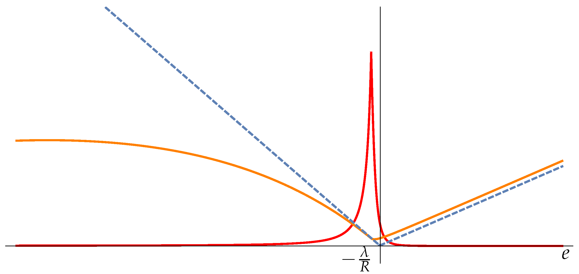
5.3. Two-Body System

In this example we consider an isolated system of two points of equal mass m subject to gravitational forces. If $x=(x_1,x_2)$, $x_i\in {\mathbb{R}}^3$, $i=1,2$ denote the positions of the two points, the potential energy is $u(x,\mathit{\lambda })={\displaystyle \frac{-\mathit{\lambda }}{|x_2-x_1|}}$, where $\mathit{\lambda }=G{m}^2$ can be considered as a parameter. A system of points interacting via gravity requires a specific description in statistical mechanics due to the long-range nature of the force, which prevents these systems from displaying the extensive character of the total energy. Also, it is known that gravitating systems exhibit the phenomenon of negative specific heat [24], a possibility that is excluded in the canonical description; see (36). Therefore, the correct statistical ensemble to adopt is the microcanonical one; see [25]. In [25], the above two-body system is modified to construct a toy model that exhibits all the features of a many-body self-gravitating system. This is obtained by imposing a short-range cutoff on the particles inter-distance $|x_2-x_1|>a$, which behaves as hard spheres of radius $a/2$, and a long-range cutoff $|x_2-x_1|<R$. This modified system displays a phase transition between phases of positive and negative specific heat when the system energy is varied. We want to discuss this mechanical system using HB thermodynamics. See also [5] for a different analysis of a two-body system with HB thermodynamics. Therefore, we compute the probability density (10) and the Fisher information for this system and discuss its ability to describe phase transitions. Using (12), we have for $e<0$,

$$H(e,\mathit{\lambda })=\{x\in {\mathbb{R}}^6:\mathit{\phi }(x,e,\mathit{\lambda })=e-u(x,\mathit{\lambda })=e+{\displaystyle \frac{\mathit{\lambda }}{|x_2-x_1|}}>0\}$$

and from (10) with $d=6$, $c={\displaystyle \frac{d}{2}}-1=2$,

$$Z(e,\mathit{\lambda })={\int }_{H(e,\mathit{\lambda })}{\mathit{\phi }}^{c}dx={\int }_{H(e,\mathit{\lambda })}{\left(e+{\displaystyle \frac{\mathit{\lambda }}{|x_2-x_1|}}\right)}^{2}d{x}_{1}d{x}_2.$$

To compute the last integral, it is useful to perform the change in variables $\chi (x_1,x_2)=(x_1,s+x_1)$, where $s=x_2-x_1$ is the inter-particle vector. We have $detd\chi =1$ and $H(e,\mathit{\lambda })=\chi (\Lambda )$ where

$$\Lambda =\{(x_1,s)\in {\mathbb{R}}^6:\left|s\right|<{\displaystyle \frac{-\mathit{\lambda }}{e}}\}={\mathbb{R}}_{x_1}^3\times B_3({\displaystyle \frac{-\mathit{\lambda }}{e}})$$

therefore, by using the change in variable and the Fubini theorem, we can write

$$Z(e,\mathit{\lambda })={\int }_{\Lambda }{\left(e+{\displaystyle \frac{\mathit{\lambda }}{\left|s\right|}}\right)}^{2}detd\chi d{x}_{1}ds={\int }_{{\mathbb{R}}_{x_1}^3}d{x}_1{\int }_{B_3({\displaystyle \frac{-\mathit{\lambda }}{e}})}{\left(e+{\displaystyle \frac{\mathit{\lambda }}{\left|s\right|}}\right)}^{2}ds.$$

The integral in $d{x}_1$ is infinite unless we assume that the particle $x_1$ is confined in a bounded region of volume V. Therefore we can write the equality above as $Z=V{Z}_s$ and, since we deal with a function radial in s we have that $Z_s$ is finite and

$$Z_s(e,\mathit{\lambda })={\int }_0^{{\displaystyle \frac{-\mathit{\lambda }}{e}}}{\left(e+{\displaystyle \frac{\mathit{\lambda }}{s}}\right)}^2{s}^{2}ds=-{\displaystyle \frac{{\alpha }_2{\mathit{\lambda }}^3}{3e}},e<0.$$

(40)

The probability density (10) is thus factorized into the product of two densities

$$p(e,\mathit{\lambda },x_1,s)d{x}_{1}ds={\displaystyle \frac{{\mathit{\phi }}^c}{Z(e,\mathit{\lambda })}}d{x}_{1}ds={\displaystyle \frac{d{x}_1}{V}}·{\displaystyle \frac{{\mathit{\phi }}^2(e,\mathit{\lambda },s)}{Z_s}}ds$$

showing that the positions of the two particles are independent random variables. Therefore we can forget about the $x_1$ particle and perform all the computations in the s variable.

If we let the energy tend to zero so that the inter-particle distance s can be arbitrarily large, we make $Z_s$ in (40), hence the microcanonical entropy of the system $S_{\mu }=lnZ$, infinite. The HB or volume entropy is

$$S=S_{\mu }+ln\langle \mathit{\phi }\rangle$$

and it is easy to see that $\langle \mathit{\phi }\rangle$ is infinite if we let the inter-particle distance s go to zero, so the entropy S is infinite when s tend to zero or to infinity, while $S_{\mu }$ is infinite only in the latter case.

Therefore, it is necessary to assume, as in [25], that there are two cutoffs $a<\left|s\right|<R$, usually with $R\gg a$, so that the two-body system is confined in a bounded region of space. Moreover, the system displays two energy scales

$$e_{min}=u\left(a\right)=-{\displaystyle \frac{\mathit{\lambda }}{a}}<0,e_R=u\left(r\right)=-{\displaystyle \frac{\mathit{\lambda }}{R}}<0$$

Also, it is stipulated in [25] that if the energy is in the range $e_{min}\le e\le e_R$, the integration in the s variable is performed between extrema a and ${\displaystyle \frac{-\mathit{\lambda }}{e}}$, while for $e\ge e_R$ the integration is between fixed extrema a and R. Due to the presence of the cutoff a, the system displays a negative specific heat phase (see again [25]).

We can now compute the temperature T, the microcanonical temperature $T_{\mu }$, and the pressure P using (21) for our system in the two energy ranges and then juxtapose the plots that have continuous junction at $e=e_R$. See Appendix A for computations. We also compute the Fisher information $g_{00}(e,\mathit{\lambda })$ from (33). See Figure 1 for the plot of T, $T_{\mu }$, and $g_{00}$.

The temperature $T=T(e,\mathit{\lambda })$ (blue curve of Figure 1) presents a gentle maximum for negative energy (point B) and a sharp minimum (point C) for a positive value of the energy. We see that for $e=e_{min}$, the temperature is zero, as in the previous example 1. The temperature curve of this simple mechanical system displays the same features of more complex and realistic models of gravitating many-particle systems: a phase (A to B) of positive specific heat followed by a phase (B to C) of negative specific heat and again a phase of positive specific heat (after C). The microcanonical temperature $T_{\mu }$ (orange curve) has a similar behavior to T. The points where the two temperature curves cross each other are the points where the specific heat $c_v$ diverges; see (24). See [25] for a physical interpretation of these phases.

We see that the Fisher information $g_{00}=g_{00}(e,\mathit{\lambda })$ (red curve of Figure 1) diverges for $e=e_{min}$ and has a peak for $e=e_R$. The divergence in $e=e_{min}$ is located at the minimum of the potential energy (due to the cutoff at $s=a$), and it is similar to the one found in the previous example 1. Here we are concerned with the assessment of the ability of Fisher information to locate the phase transitions at B and C. It seems that the phase transition in B is not detected, and the one in C is not exactly located. This is due to the presence of the cutoffs $a<s<R$ (which are essential for the existence of the negative specific heat phase). As far as the phase transition in B is concerned, the shape of the curve of temperature T does not change with a, and in the limit $a\to 0$, entropy S becomes infinite. On the other hand, the microcanonical entropy $S_{\mu }=lnZ$ is defined for $a=0$, and the curve of the microcanonical temperature computed for $a=0$ (dashed line of Figure 2) does not show the phase A to B of positive specific heat. Therefore, for $a=0$, the phase transition in B is removed in the microcanonical description of the system, while the remaining one is detected by the divergence of Fisher information.

We will show that if the bounds are removed, letting $a\to 0$ and $R\to +\infty$, the minimum C and the peak in Fisher information $g_{00}$ coincide at $e=0$. In fact, the energy corresponding to point C can be determined using the condition $\partial T(e,\mathit{\lambda })/\partial e=0$. By computing $\partial T(e,\mathit{\lambda })/\partial e=0$ at the leading order in $1\gg a/R$ we deduce that the minimum in C in Figure 1 is located at

$$e_2^{*}={\displaystyle \frac{\mathit{\lambda }}{R}}\sqrt[3]{6lnR}.$$

The peak of Fisher information is located at $e=e_R=-\mathit{\lambda }/R$, and its height is

$$g_{00}(-{\displaystyle \frac{\mathit{\lambda }}{R}},\mathit{\lambda })={\displaystyle \frac{3R^4}{{\mathit{\lambda }}^2{(a-R)}^2}}\simeq 3{({\displaystyle \frac{R}{\mathit{\lambda }}})}^2$$

In the limit $R\to +\infty$ both $e_R$ and $e_2^{*}$ tends to 0. So we can say that the divergence of Fisher information $g_{00}$ correctly detects the phase transition from negative to positive specific heat located at $e=0$.

6. Conclusions

The formulation of HB thermodynamics defines the analogs of temperature, pressure, and entropy for a mechanical system whose potential energy depends on a parameter $\mathit{\lambda }$. This scheme has been generalized to n degree-of-freedom systems with multiple parameters, but generalization to an infinite number of degrees of freedom (and hence the operation of thermodynamic limit) seems to be beyond the possibilities of the theory. Therefore, it is interesting (and it is the aim of this work) to ask if the thermodynamic description of these mechanical systems is capable of displaying different patterns of organization (driven by qualitative changes in the underlying dynamics ) and if these patterns can be signaled by an order parameter. Given the probabilistic nature of the theory, it has been natural to investigate if the HB thermodynamic scheme can be read as a statistical model and to compute the associated Fisher matrix, which has previously been used in the literature to describe systems that are of a more general nature than those considered in statistical mechanics. We have shown with some paradigmatic examples that there are cases in which the Fisher information computed from HB thermodynamics is capable of locating phase transitions in the generalized sense exposed above.

References

1. Helmholtz, H. Principien der Statik Monocyklischer Systeme. Crelle’s J. 1884, 97S, 111–140, reprinted in Wissenschaftliche Abhandlungen; Walter de Gruyter GmbH: Leipzig, Germany, 1895; Volume III, pp. 142–162+179–202. [Google Scholar] [CrossRef]
2. Helmholtz, H. Studien zur Statik Monocyklischer Systeme; Akademie der Wissenschaften zu Berlin: Berlin, Germany, 1884; pp. 159–177, reprinted in Wissenschaftliche Abhandlungen; Walter de Gruyter GmbH: Leipzig, Germany, 1895; Volume III, pp. 163–172+173–178. [Google Scholar]
3. Boltzmann, L. Uber die Eigenschaften monozyklischer und anderer damit verwandter Systeme. Crelle’s J. 1884, 98, S68–S94, reprinted in Wissenschaftliche Abhandlungen von Ludwig Boltzmann; Hasenöhrl, F., Ed.; Johann Ambrosius Barth: Leipzig, Germany, 1909; Band III, p. 122; reprinted in Wissenschaftliche Abhandlungen von Ludwig Boltzmann; Chelsea Publ. Company: New York, NY, USA, 1968. [Google Scholar]
4. Gibbs, J.W. Elementary Principles in Statistical Mechanics: Developed with Especial Reference to the Rational Foundations of Thermodynamics; C. Scribner’s Sons: New York, NY, USA, 1902. [Google Scholar]
5. Gallavotti, G. Statistical Mechanics. A Short Treatise; Texts and Monographs in Physics; Springer: Berlin/Heidelberg, Germany, 1999. [Google Scholar]
6. Porporato, A.; Rondoni, L. Deterministic engines extending Helmholtz thermodynamics. Phys. A Stat. Mech. Its Appl. 2024, 640, 129700. [Google Scholar] [CrossRef]
7. Cardin, F.; Favretti, M. On the Helmholtz-Boltzmann thermodynamics of mechanical systems. Contin. Mech. Thermodyn. 2004, 16, 15–29. [Google Scholar] [CrossRef]
8. Campisi, M. On the mechanical foundations of thermodynamics: The generalized Helmholtz theorem. Stud. Hist. Philos. Sci. Part Stud. Hist. Philos. Mod. Phys. 2005, 36, 275–290. [Google Scholar] [CrossRef]
9. Fisher, R.A. On the mathematical foundations of theoretical statistics. Philos. Trans. R. Soc. Lond. Ser. A 1922, 222, 309–368. [Google Scholar]
10. Rao, C.R. Information and the accuracy attainable in the estimation of statistical parameters. In Breakthroughs in Statistics; Springer: New York, NY, USA, 1992; pp. 235–247. [Google Scholar]
11. Amari, S.; Nagaoka, H. Methods of Information Geometry; AMS and Oxford University Press: Oxford, UK, 2000. [Google Scholar]
12. Amari, S. Information Geometry and Its Applications; Springer: Berlin/Heidelberg, Germany, 2016; Volume 194. [Google Scholar]
13. Calin, O.; Udriste, C. Geometric Modeling in Probability and Statistics; Springer: Berlin/Heidelberg, Germany, 2014. [Google Scholar]
14. Crooks, G.E. Fisher Information and Statistical Mechanics. Tech. Note 008v4. 2012. Available online: http://threeplusone.com/fisher (accessed on 1 July 2025).
15. Arnold, J.; Lörch, N.; Holtorf, F.; Schäfer, F. Machine learning phase transitions: Connections to the Fisher information. arXiv 2023, arXiv:2311.10710. [Google Scholar]
16. Brunel, N.; Nadal, J.P. Mutual information, Fisher information, and population coding. Neural Comput. 1998, 10, 1731–1757. [Google Scholar] [CrossRef]
17. Petz, D. Quantum Information Theory and Quantum Statistics; Springer: Berlin/Heidelberg, Germany, 2008. [Google Scholar]
18. Prokopenko, M.; Lizier, J.T.; Obst, O.; Wang, X.R. Relating Fisher information to order parameters. Phys. Rev. E 2011, 84, 041116. [Google Scholar] [CrossRef]
19. Huang, K. Statistical Mechanics; John Wiley & Sons: Hoboken, NJ, USA, 2008. [Google Scholar]
20. Favretti, M. Geometry and control of thermodynamic systems described by generalized exponential families. J. Geom. Phys. 2022, 176, 104497. [Google Scholar] [CrossRef]
21. Favretti, M. Exponential Families with External Parameters. Entropy 2022, 24, 698. [Google Scholar] [CrossRef]
22. Dauxois, T.; Ruffo, S.; Arimondo, E.; Wilkens, M. Dynamics and Thermodynamics of Systems with Long-Range Interactions: An Introduction; Springer: Berlin/Heidelberg, Germany, 2002. [Google Scholar]
23. Campa, A.; Dauxois, T.; Ruffo, S. Statistical mechanics and dynamics of solvable models with long-range interactions. Phys. Rep. 2009, 480, 57–159. [Google Scholar] [CrossRef]
24. Thirring, W. Systems with negative specific heat. Z. Phys. 1970, 235, 339. [Google Scholar] [CrossRef]
25. Padmanabhan, T. Statistical mechanics of gravitating systems. Phys. Rep. 1990, 188, 285–362. [Google Scholar] [CrossRef]
Figure 1. Plot of Fisher information g 00 (red curve), temperature T (blue curve), and microcanonical temperature T μ (orange curve) as a function of the energy e.
Foundations 05 00024 g001
Figure 2. Plot of Fisher information g 00 (red curve), microcanonical temperature T μ (orange curve), and microcanonical temperature for a = 0 (dashed curve) as a function of the energy e. In the a = 0 case, the phase of negative specific heat is not present, and the remaining phase transition is located at e = 0 . Note that for greater clarity, the plot is not in the whole energy range e > λ / a .
Foundations 05 00024 g002
Disclaimer/Publisher’s Note: The statements, opinions and data contained in all publications are solely those of the individual author(s) and contributor(s) and not of MDPI and/or the editor(s). MDPI and/or the editor(s) disclaim responsibility for any injury to people or property resulting from any ideas, methods, instructions or products referred to in the content.