Abstract
The rising demand for both water and energy has intensified the urgency of addressing the water–energy nexus. Energy is required for water treatment and distribution, and energy production processes require water. The increasing demand for energy requires substantial amounts of water, primarily for cooling. The emergence of new persistent contaminants has necessitated the use of advanced, energy-intensive water treatment methods. Coupled with the energy demands of water distribution, this has significantly strained the already limited energy resources. Regrettably, no straightforward, universal model exists for estimating water usage and energy consumption in power and water treatment plants, respectively. Current approaches rely on data from direct surveys of plant operators, which are often unreliable and incomplete. This has significantly undermined the efficiency of the plants as these surveys often miss out on complex interactions, lack robust predictive power and fail to account for dynamic temporal changes. The study thus aims to evaluate the potential of mathematical modeling and simulation in the water–energy nexus. It formulates a mathematical framework and subsequent simulation in Java programming to estimate the water use in hydroelectric power and geothermal energy, the energy consumption of the advanced water treatment processes focusing on advanced oxidation processes and membrane separation processes and energy demands of water distribution. The importance of mathematical modeling and simulation in the water–energy nexus has been extensively discussed. The paper then addresses the challenges and prospects and provides a way forward. The findings of this study strongly demonstrate the effectiveness of mathematical modeling and simulation in navigating the complexities of the water–energy nexus.
1. Introduction
The intricate and intertwined interrelationship between water and energy often referred to as the water–energy nexus is becoming increasingly important as the demand for both resources rises [1,2]. The rapid global economic expansion and the rising of living standards, accompanied by swift industrial growth have resulted to increase in the global energy demand which is projected to further exacerbate by a 15% increase in the near future [3]. To meet this growing energy demand, alternative sources of energy generation are being explored globally. Chief among these are the renewable energy technologies due to the growing awareness of depletion of non-renewable energy technologies and destructive impact of fossil fuels particularly in relation to climate change as the world aims for net zero emissions by 2050.
The shift to renewable energy technologies, now at a 38% of the global energy consumption [4] and expected to increase in the coming years, has put significant pressure on the water resources in the regions where they are situated since they require substantial amount of water primarily for cooling and some consumed through evaporation. This coincidentally comes at a time when the world is facing a water crisis in alarming proportions characterized by water scarcity and deterioration of water quality [5]. Water purification emerges as a vital component in addressing the crisis with variety of water treatment methods being examined worldwide [6]. The emergence of new persistent contaminants such as pharmaceutical and personal care products (PPCPs), dyes, heavy metals and radioactive substances have necessitated the utilization of advanced, energy intensive water treatment methods specially advanced oxidation processes (AOPs) and membrane separation processes [7]. Coupled with the energy demands of water distribution, this has put significant strain on the already limited energy resources further increasing the global energy demand. Hence, understanding both the water footprint of renewable energy technologies and energy consumption of advanced water treatment methods becomes a mandatory concern in order to make informed decisions about the location of the plants and optimal utilization of these scarce resources [8]. This aligns seamlessly with the global sustainable development goals (SDGs), particularly SDG 6 (universal access to clean water) and SDG 7 (affordable, reliable and sustainable energy for all). Unfortunately, there is no straightforward and universally applicable model for assessing water usage and energy consumption in power and water treatment plants.
Current techniques rely on plant operator survey data, which is often incomplete and unreliable. This has compromised the efficiency of the plants, with most of them operating significantly below their optimal capacity [9]. The plant operator surveys while valuable in gathering operational insights often fall short in capturing the complex interactions and feedback loops in the water–energy nexus. These surveys miss important variables and relationships resulting in oversimplified analyses that do not reflect the dynamics of plant operations. Additionally, they lack robust predictive power, making it challenging to anticipate future performance under varying conditions. The temporal changes with the plant such as fluctuations in water use, energy consumption and changing environmental conditions are usually not adequately accounted for, resulting in inefficient operations and suboptimal optimization procedures [10]. This underscores the pressing need for mathematical modeling and simulation which provides a more comprehensive understanding of the water–energy nexus, enabling operators to simulate different scenarios, predict outcomes, identify optimal strategies for improving efficiency and performance and provides a quantitative basis for making informed decisions.
The present study evaluates the potential of mathematical modeling and simulation in the water energy nexus. The second section provides an overview of the water–energy nexus. Section 3 discusses the commonly utilized mathematical models and simulation approaches. Section 4 and Section 5 focus on the application of mathematical modeling and simulation in the water–energy nexus. The formulation of the mathematical framework and subsequent simulation in Java programming to estimate the water use in hydropower and geothermal energy is presented. The energy consumption of the advanced water treatment processes, particularly the advanced oxidation processes (AOPs) and membrane separation processes and water distribution considering the hydrodynamics and hydraulic transients are discussed. Section 6 gives the importance of mathematical modeling and simulation in the water–energy nexus. Section 7 addresses the challenges arising and potential benefits of applying mathematical modeling and simulation to the water–energy nexus. Finally, Section 8 gives the conclusions and future research directions.
2. The Water–Energy Nexus
The water–energy nexus is an inseparable interdependence between water and energy [1]. Every stage of the water cycle from water purification, distribution and wastewater treatment consumes energy. Conversely, every power source demands water in one form or another for fuel processing, thermoelectric cooling and evaporation. Figure 1 summarizes the water energy nexus. The water footprint of energy generation technologies refers to the ratio of the amount of fresh water consumed in energy production to the electricity generated.
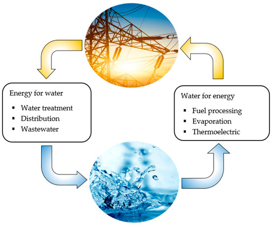
Figure 1.
The water–energy nexus.
The water consumed, utilized directly for power consumption, cooling processes or other operational processes, varies depending on the type of fuel used. Table 1 summarizes the average water footprint of various energy production processes.

Table 1.
Water footprint of major energy generation technologies.
The energy consumption of water treatment systems constitute the amount of energy required to process raw water into potable water for distribution to consumers and treating wastewater before discharging it back to the environment [18]. Depending with the technology utilized, plant design and desired quality of the effluent treated water, wastewater treatment plants consumed about 0.5–2 kWh/m3 of treated water [19] with conventional water treatment plants operating at 0.11–0.91 kWh/m3 [20]. Table 2 summarizes the average energy consumption of major water treatment processes.
Table 2.
Energy consumption of major water treatment processes.
3. Mathematical Modelling and Simulation
3.1. Mathematical Modeling
Mathematical modeling is the process of translating real-world problems or phenomenon into a mathematical representation using equations, functions and graphs [26,27]. Table 3 shows some of the most utilized mathematical models.
Table 3.
Commonly utilized mathematical models.
3.2. Simulation
Process simulation refers to a virtual imitation of a real-world process or system designed to study its behavior under controlled conditions [33]. There are two approaches to simulation: programming-based simulation and software-based simulation. Programming based simulation involves writing a custom code to create simulations. The user programs simulation from scratch using either of the diverse programming languages such as C, C++, Java and Python. This approach is best for highly specialized simulations, when specific control over the simulation process is needed, or when integrating with other custom software [34]. Software-based simulation involves using pre-built simulation software tools that provide user interfaces and built-in functionalities to create simulations without writing extensive code, usually ideal for standard simulations and when rapid prototyping is required [35,36].
4. Application of Mathematical Modelling to the Water–Energy Nexus
The application of mathematical modeling to the water–energy nexus, helps us to understand the intricate connection between water and energy systems providing a quantitaive framework for analysis, optimization, prediction and ensuring sustainable and equitable allocation of these scarce resources [37]. We thus utilize mathematical modeling to estimate the water consumption in renewable energy technologies like hydroelectric power and geothermal energy. Additionally, we analyze the energy consumption of the advanced water treatment such as advanced oxidation processes (AOPs) and membrane separation processes as well as the energy associated water distribution considering the hydrodynamics and hydraulic transients.
4.1. Water Footprint of Renewable Energy Technologies
A mathematical analysis of the renewable energy water footprint provides a quantitative basis for facilitating scenario analysis and informed decision-making, ensuring these technologies are truly sustainable and contribute to a more water-secure future [38]. The following is the water footprint mathematical modeling of major renewable energy technologies.
4.1.1. Hydroelectric Power
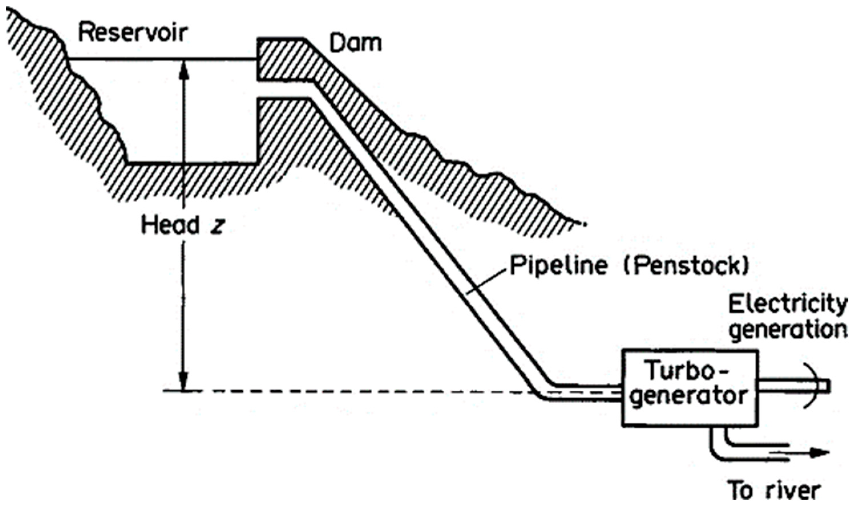
Hydroelectric power is a renewable energy source that harnesses the potential and kinetic energy of flowing water to generate electricity [39]. Water is released from the reservoir through a controlled opening in the dam and enters a large pipe called the penstock, which channels the water towards the turbine. The water, under high pressure, strikes the blades of the turbine initiating rotation. A generator coupled with the rotating turbine converts the mechanical energy into electrical energy, which is transmitted through cables to a substation, transformed and distributed to the electrical grid. Figure 2 shows the schematic of a hydroelectric power plant.
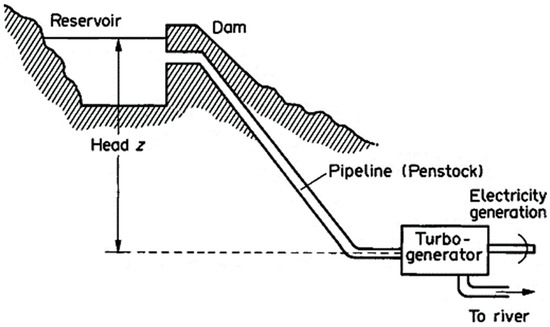
Figure 2.
Schematic of a hydroelectric power plant reprinted with permission from [40] © Elsevier 1994.
Hydroelectric power plants do not consume water directly in the process of generating electricity as the water simply passes through the turbines and continues downstream. However, the large reservoir created behind the dam disrupts the local water balance by significantly increasing the surface area exposed to evaporation. This leads to greater water loss to the atmosphere than would occur in a natural river flow. This evaporative loss of water is the contributor to the hydroelectric power water footprint as it represents the permanent reduction in the water available for the downstream ecosystems. The water footprint of hydroelectric power is thus the ratio of the amount of water lost through evaporation from the reservoir to the amount of energy generated mathematically expressed as [41,42],
where is volume of water evaporated from the reservoir annually (m3/yr.) and E is the energy generated (GJ/yr.),
where is reservoir area (ha) and is the daily evaporation (mm/day) given by the Penman–Monteith equation,
where is the latent heat of evaporation at air temperature, is the net radiation, is the change in heat storage of the water body, is the psychometric constant, is the slope of the temperature saturation water vapor curve, and are the saturated vapor pressure at water temperature and air temperature respectively and is calculated from wind function. The latent heat of evaporation, (MJ/Kg) at (°C) air temperature and the psychometric constant, (kPa/°C), are calculated from Equations (4) and (5),
where is the atmospheric pressure in kPa, which varies with elevation above the sea level, and (m) is given by the expression
The saturated vapor pressure at water temperature, , air temperature, , and the slope of the temperature saturation water vapor, , are calculated from Equations (7)–(9)
where and are the water surface temperature (°C) and air temperature (°C) respectively. The wind function is calculated from wind speed at 10 m, (m/s), and the equivalent area, (km2). as shown,
The net radiation, , is given by the difference between the net incoming short-wave radiation, (MJ m−2 day−1), and the net outgoing long-wave radiation .
The net incoming short waves and outgoing long-wave radiation are mostly determined experimentally using net radiometers. Nevertheless, theoretical calculations have been carried out and discussed by various studies [41,43,44]. The change in the heat storage of a water body, , is calculated from the change in temperature difference in the water of successive measurements
where is the density of water (1000 kg m−3), is the specific heat of water (0.0042 MJ kg−1 K−1) and is the depth of water in the reservoir (m).
4.1.2. Geothermal Energy
Geothermal energy is a renewable energy source that uses heat stored within the earth’s crust generated by radioactive decay and residual heat during planetary formation to produce electricity [45]. Depending on the driving mechanism of the turbine, temperature and pressure requirements, geothermal power plants can be classified into three categories: dry steam, flash steam and binary cycle. Dry steam power plants use steam (235 °C) directly to drive turbines, which generate electricity. Flash steam power plants utilize hot water from the ground (180 °C) pumped under high pressure to the surface where its pressure is reduced causing the water to be flashed into steam which then drives a turbine to generate electricity. Binary cycle power plants use either steam, hot water or both to heat secondary fluids such as ammonia to vapor which drives a turbine to generate electricity, making it one of the most used and versatile techniques, operating at relatively low temperatures. Figure 3 shows the schematic of a binary cycle geothermal power plant.
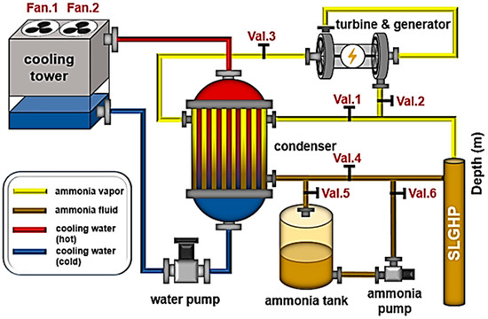
Figure 3.
Schematic of a binary cycle geothermal power plant reprinted with permission from [46] © Royal Society of Chemistry 2024.
The water footprint of geothermal energy refers to the amount of water consumed through cooling which can be either once-through cooling or evaporation cooling (evaporation and blowdown) to the net electricity generated [47,48]. A non-cooling process intensity coefficient, , is usually added to account for the water use in all the non-cooling processes in the plant
where is the rate of water consumption during cooling and is the net electricity generated. Consider the heat balance around the cooling system,
where is the heat load of the cooling system, is the rate of thermal energy input into the plant, is the net efficiency and is the fraction of heat lost to sinks besides the cooling system mathematically calculated as
where is the rate of heat lost to sinks other than the cooling system. The water footprint of a geothermal power plant varies depending on the type of cooling system employed, either once-through cooling or evaporation cooling. Once-through cooling, also referred to as open-loop cooling, involves drawing water from a water body, passing it through a heat exchanger where it absorbs heat and discharging it back to the water body, relatively warmer. The water footprint of the cooling system is due to the increased evaporation, attributed by the elevated temperatures of the discharge water. Consider the cooling water flowrate of a once-through cooling system, mathematically expressed as,
where is the temperature difference between the inlet and outlet cooling water and is the specific heat of water (4184 J kg−1 K−1 at 20 °C). Substituting Equation (14) into (16), we obtain
Equation (19) is the water footprint equation for a once-through cooling system. An evaporative cooling system uses a recirculating loop of cooling water and flow of air to effectively cool the geothermal or secondary fluid. It operates based on the principle that evaporation of water removes heat and some water must be replaced (blowdown) to control the concentration of dissolved materials in the water. The total amount of water consumed during the process is thus water lost through both evaporation and blowdown. The rate of water consumption through evaporation is expressed as,
where is the latent heat of vaporization (2454 kJ kg−1 at 20 °C) and represents the fraction of heat load rejects through sensible heat transfer, mathematically expressed as,
The evaporation coefficient, is related to the cooling tower temperature range by the equation, based on the industry rules of the thumb. These simplifying assumptions implicitly assume that is a constant. The rate of water consumption through blowdown is related to the rate of water lost through evaporation in terms of the number of cycles of concentration, , a parameter that determines how many times water is reused before blowdown occurs usually in the range of 2–10 for most geothermal plants.
The summation of Equations (20) and (22) gives the total amount of water consumed in an evaporative cooling system.
Substituting Equations (11) into (16),
Equation (29) is the water footprint equation for an evaporating cooling system.
4.2. Energy Consumption in Advanced Water Treatment and Distribution
Advanced water treatment processes such as advanced oxidation processes (AOPs) and membrane separation, while effective in eliminating persistent contaminants and improving water quality, come with significant energy consumption. Thus, understanding the energy requirements of advanced water treatment processes is essential in improving the sustainability and overall efficiency of water treatment plants [18]. We thus utilize mathematical modeling to understand the energy requirements of the advanced oxidation processes (AOPs) and membrane separation processes as well as the energy demands of water distribution.
4.2.1. Advanced Oxidation Processes (AOPs)
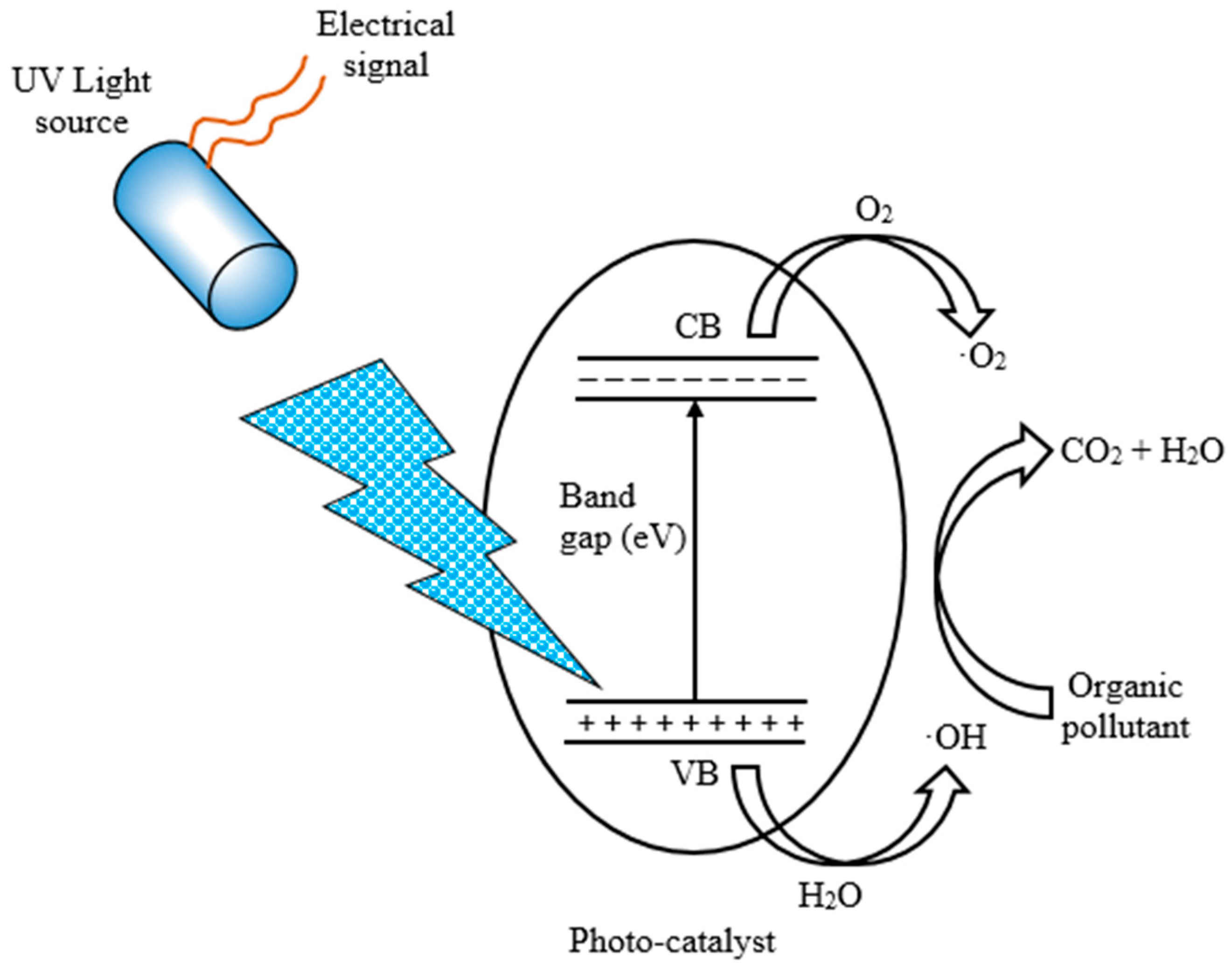
AOPs use highly reactive oxidative species called hydroxyl radicals to break down and eliminate contaminants in the presence of radiation, mostly UV from either a mercury or a xenon lamp. They include the photo-Fenton process, the photo-catalysis and ozonation processes, which use an iron (Fe2+) catalyst and a hydrogen peroxide oxidant, a photo-catalyst such as TiO2 and ozone (O3), and a powerful oxidizing agent, respectively, to effectively eliminate organic pollutants in the presence of UV radiation [49]. Consider the schematic of photocatalytic degradation of organic pollutants that occurs in the presence of UV radiation from either a mercury or a xenon lamp as shown in Figure 4.

Figure 4.
UV irradiation photocatalytic degradation process.
The UV light source receives electrical energy from a power supply which is converted to thermal energy in the lamp electrodes emitting electrons through thermionic emissions which are accelerated across the lamp because of the applied electric field. The accelerated electrons collide with gas atoms such as mercury vapor or a noble gas (Xenon) exciting the electrons in the atoms to higher energy states. As the electrons transition back to their lower energy states, they emit photons in the UV range [50,51]. The emitted UV photons travel to the photo-catalyst to initiate the photocatalytic degradation of the organic pollutant through the creation of electron–hole pairs. Consider the general equation for energy conversion in the UV lamp,
where is the power supply, t is time, is the number of photons emitted, is the Planck’s constant and is the overall efficiency, which is given by
where is the electrical efficiency, which takes into account the ohmic and thermal losses, and is the excitation efficiency, which considers the fraction of collisions between electrons and gas atoms that will result in the desired excitation to higher energy levels, and is the irradiation efficiency, which accounts for the fraction of excited states that result in UV photon emission. The excitation efficiency is often calculated from the Maxwell–Boltzmann distribution, which gives the probability of finding a particle with energy , at a given temperature [52]
where is probability distribution density function of particle energies in a gas at thermal equilibrium, is the particle mass, is the Boltzmann constant and T is the thermodynamic temperature. Incorporating the inverse square law of radiation, which states that the intensity of radiation diminishes proportionally to the square of the distance from the UV lamp [53] into Equation (30).
Equation (34) is the general equation for the energy requirements for a UV photocatalytic degradation of organic pollutants.
4.2.2. Membrane Separation Processes
Membrane separation processes utilize a semi-permeable membrane with tiny pores to selectively remove pollutant particles and macromolecules from water. Pressure difference is the main driving mechanism for most membrane separation. Figure 5 illustrates the membrane separation processes [54].
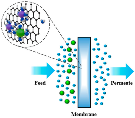
Figure 5.
Membrane separation processes.
The membranes are classified based on their pore size into microfiltration, ultrafiltration, nano-filtration and reverse osmosis. Microfiltration uses 0.1–10 µm pore size membranes and pressure difference as the main driving mechanism to effectively remove turbidity in water. Ultrafiltration uses 0.01–0.1 µm pore size membranes and pressure difference to remove particles from water. Nano-filtration is a charged 0.001–0.01 µm pore size charged membrane to remove ions from water. Reverse osmosis utilizes less than 0.001 µm pore size membranes and pressure difference against osmotic pressure to remove molecules from water. In a steady state process, water is pressurized from a low pressure to a high pressure using a circulation pump which maintains a high crossflow velocity. The power of the circulation pump is calculated based on the geometry of the path where the water flows. Two geometries are usually employed: rectangular (spiral wound, plate and frame) and cylindrical (hollow fibers, capillaries, tubular systems) [55,56]. Consider the general energy balance equation for a reversible steady-state fluid flow:
Assuming negligible kinetic and potential energy,
For a compressible fluid under isentropic conditions:
However, the actual work is usually higher since the process occurs irreversibly and thus some work is wasted. We define thermodynamic efficiency () as the ratio of the minimum to the actual work. The efficiency is usually between 0.5 and 0.8 [55]. Thus:
Energy is defined as work per unit time
The Hagen–Poiseuille equation can describe the pressure drop for an incompressible Newtonian fluid. Thus, for a rectangular geometry:
For cylindrical geometry:
4.2.3. Water Distribution Systems
Water distribution systems are facilities that ensure the supply of clean drinking water to the final consumers.
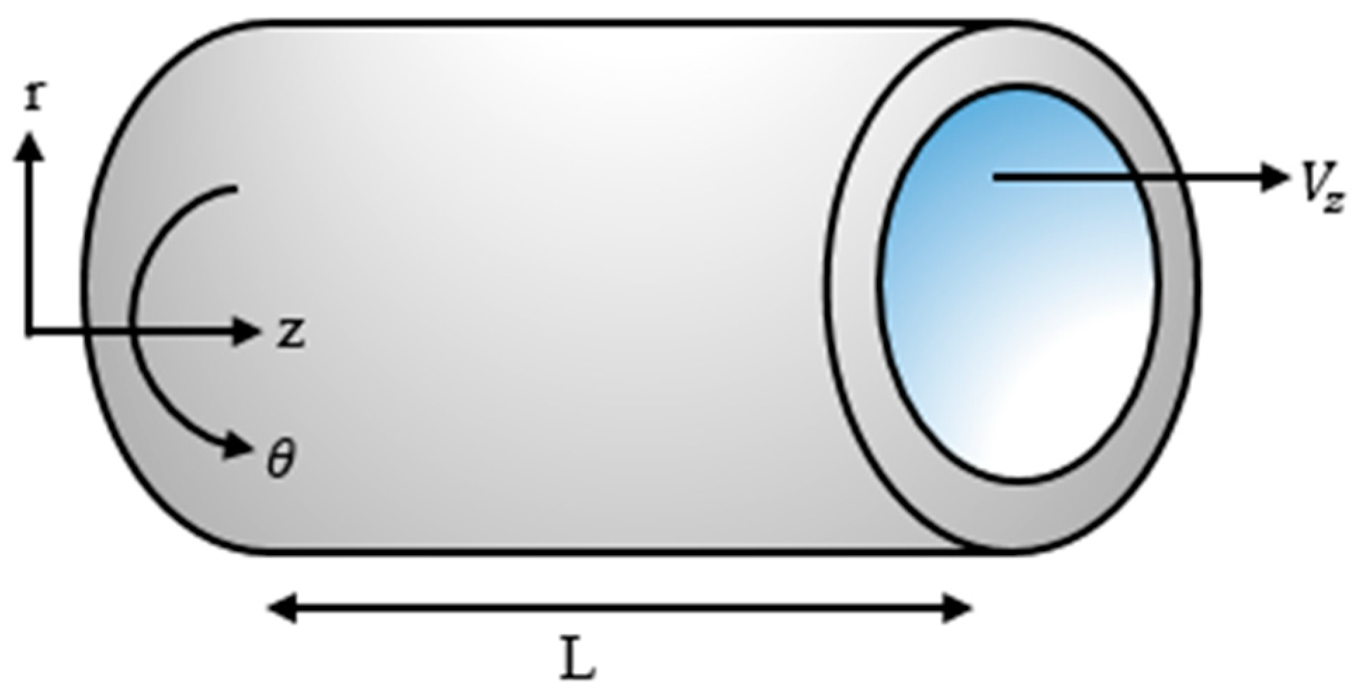
The operation of these systems, however, requires significant energy consumption, which poses a problem on the already rising energy demand and strain on the limited energy resources [57]. Thus, understanding the energy dynamics of water distribution is essential in improving efficiency, reducing costs and minimizing the environmental footprint of water utilities. The mathematical modeling and simulation presented here on the energy consumption of water distribution is carried out by considering the energy required in pumping water accounting for the losses due to frictional drag between the water and the pipe walls and losses due to hydraulic transient caused by the rapid fluctuation of pressure and velocity. Consider the flow of water through a conduit as shown in Figure 6. To understand the energy consumption of water distribution, we first model the flow of water through a conduit by solving the Navier–Stokes equations in cylindrical coordinates.

Figure 6.
Flow of water through a conduit.
We assume that the flow is steady with negligible entrance effects, resulting in a developed flow in a single coordinate (z) direction. Additionally, the flow is circumferentially symmetric, so properties do not vary in the θ direction. The no-slip boundary condition is invoked such that the velocity of the fluid is zero at the walls of the conduit and approaches infinity towards the center of the tube. The equations simplify to:
Solving the velocity profile and inserting the boundary conditions we obtain:
The volumetric flowrate is calculated from the velocity profile
The equation changes based on the main driving mechanisms that can be Poiseuille, gravitational or both based on the geometry of the channel. The power required for pumping is given by
where is the specific weight of the fluid and is the pump head calculated as shown by considering the static head, pressure head and losses due to frictional drag and hydraulic transients,
where is the total equivalent length, is the fluid velocity, is the gravitational constant, is the fanning friction factor, is the initial flow velocity through a valve and is pressure wave speed given by
where is the fluid bulk modulus of elasticity, is the conduit inside diameter, e is the wall thickness and is the material of the conduit wall Young’s modulus of elasticity. Parameter for a pipe fitted with expansion joints throughout. The fanning friction factor f is calculated for laminar flow as
where is the Reynolds number. For turbulent flows, the fanning friction factor is calculated from the von Kármán equation and the Colebrook and White expression shown in Equations (59) and (60) for smooth and rough pipes, respectively.
are is the relative roughness.
5. Process Simulation in the Water–Energy Nexus
With the growing complexity of modern systems, simulation has become indispensable for analysis and improving the water–energy nexus. More precisely, programming-based simulation allows engineers to model real-world scenarios, predict outcomes and explore trade-offs between water and energy ranging from the water footprint of energy production technologies such as hydropower and geothermal energy to assessing the energy consumption in advanced water treatment and water distribution systems. We have thus utilized programming-based simulation in Java to model and visualize the effects of various parameters in the water–energy nexus.
5.1. Simulation of Hydroelectric Power Water Footprint
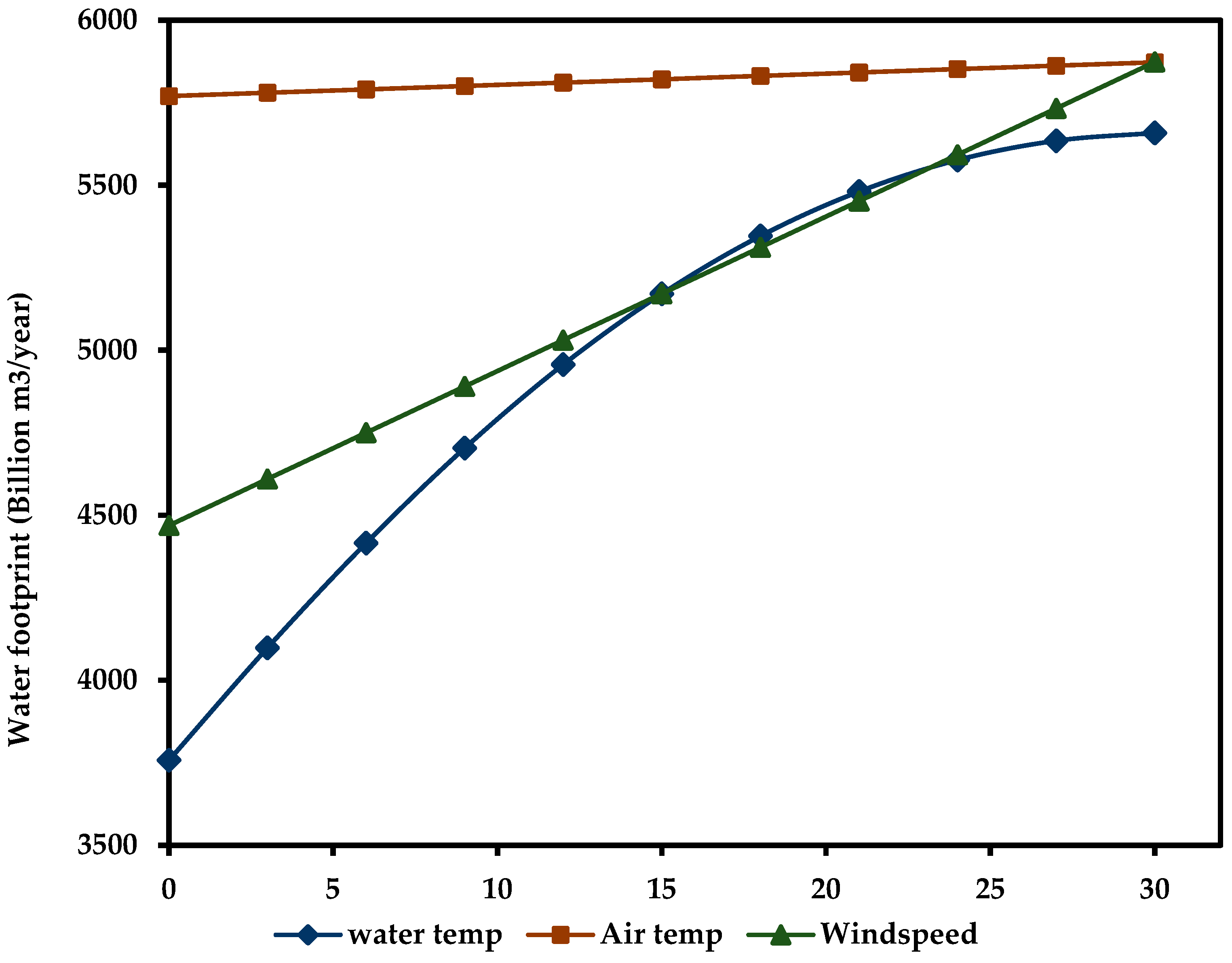
The hydropower mathematical model and subsequent simulation were applied to the 2080MW Hoover Dam hydroelectric power plant between Nevada and Arizona in the Black Canyon of the Colorado River [58] to investigate the effect of air temperature, water temperature and wind speed on the water footprint. The Hoover Dam is one of the most iconic and well-known hydroelectric power plants in the world with a long history of power generation. It is in the arid region of the southwestern United States where water management is critical. The reservoir behind the dam, Lake Mead faces significant evaporation due to high temperatures making it an ideal case scenario for analyzing the water footprint of large hydroelectric power plants. Figure 7 shows the output of the simulation. As wind speed increases across the Hoover Dam, which is at an average ambient temperature of 30 °C at the time of analysis (month of June), air saturated with water vapor is removed more efficiently allowing for more water vapor to escape to the atmosphere and thus an increase in the water footprint [59]. Conversely, the increase in the temperature difference between air and water varies proportional to the water footprint.
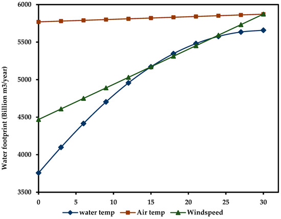
Figure 7.
Simulation of the effect of water temperature, air temperature and wind speed on the Hoover Dam hydroelectric power water footprint.
5.2. Simulation of Geothermal Energy Water Footprint
The geothermal energy mathematical model and simulation were utilized to investigate the effect of the number of cycles of concentration on the geothermal energy water footprint. The cycles of concentration are important parameters in most geothermal power plants, particularly those using cooling water tower systems that help manage water efficiency and minimize environmental impact [60]. It refers to the ratio of the concentration of impurities such as minerals and salts in the cooling water compared to the concentration in the make-up water. Figure 8 shows the output of the simulation.
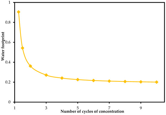
Figure 8.
Simulation of the effect of the number of cycles of concentration on the geothermal energy water footprint.
A high number of cycles of concentration translates to a lower water footprint, which means the cooling system is reusing the same water for more cycles reducing water consumption. While this is advantageous, it increases the concentration of dissolved salts, which can lead to scaling, corrosion or fouling of the cooling system. Conversely, a low number of concentration cycles results in a higher water footprint, approaching infinity as the number of cycles goes to one. As such, optimization techniques are demanded to minimize water consumption while ensuring the safety of equipment against scaling and fouling-related issues with most geothermal power plants operating between 3 and 7 cycles.
5.3. Simulation of Energy Consumption in Advanced Oxidation Processes
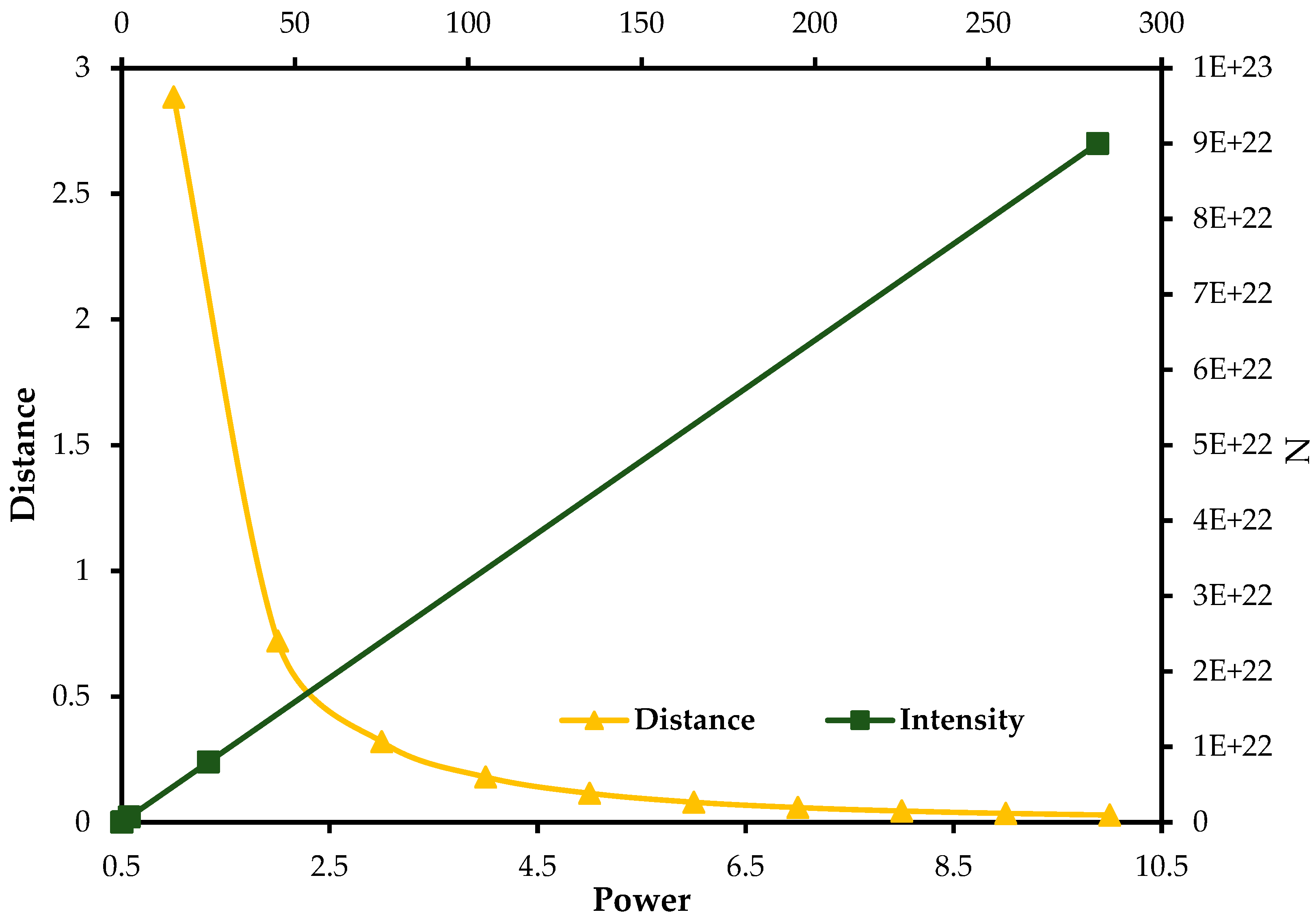
The mathematical model and subsequent simulation wer applied to investigate the effect of distance from a UV source and light intensity (number of photons) on the power requirements of UV mercury lamp utilized in the photocatalytic degradation of natural organic matter [61] in water using the silver-doped titanium dioxide (Ag-TiO2) nanocomposite photo-catalyst. Figure 9 shows the output of the simulation.
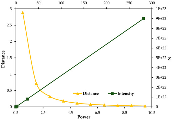
Figure 9.
Simulation of the effect of UV light source distance and intensity on the power requirements of UV mercury lamp for the Ag-TiO2 photo-catalysis.
The intensity of radiation weakens proportionally to the square of distance from the source, as the distance between the UV lamp and the photo-catalyst increases, the intensity decreases rapidly, potentially requiring higher power input to achieve the desired photocatalytic degradation efficiency. On the other hand, reducing the lamp-to-photocatalyst distance will increase the intensity of the radiation, hence necessitating power adjustments to avoid overexposure and energy waste. Rigorous optimization producers are thus required to achieve the best photocatalytic efficiency at minimal energy consumption.
5.4. Simulation of Energy Consumption in Membrane Separation Processes
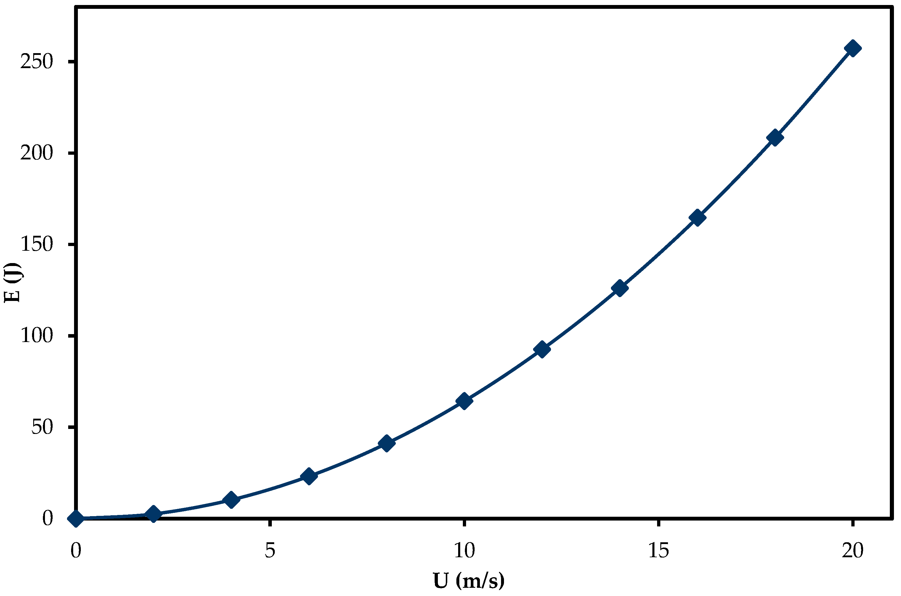
The mathematical model and subsequent simulation were applied to investigate the required crossflow velocity on energy consumption in the desalination of brackish water [62,63] using a hollow fiber reverse osmosis membrane. Figure 10 shows the output of the simulation. Reverse osmosis is one of the most efficient and widely used technologies for desalination and water purification. Of particular interest, the hollow fiber reverse osmosis systems have gained much attention in recent times, due to their high surface-area-to-volume ratio, compact design and high filtration capacity. However, the energy demands of this process are a significant concern, especially in large-scale desalination plants where operational costs are heavily influenced by energy requirements. One critical factor influencing the performance and energy efficiency of these RO systems is the cross-flow velocity across the membrane. Thus, understanding the cross-flow velocity on the energy requirements of RO systems is essential for maintaining high operation efficiency at minimum energy consumption.
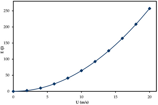
Figure 10.
Simulation of the effect of crossflow velocity on the energy requirements of a hollow fiber reverse osmosis membrane.
5.5. Simulation of the Water Distribution Energy Demands
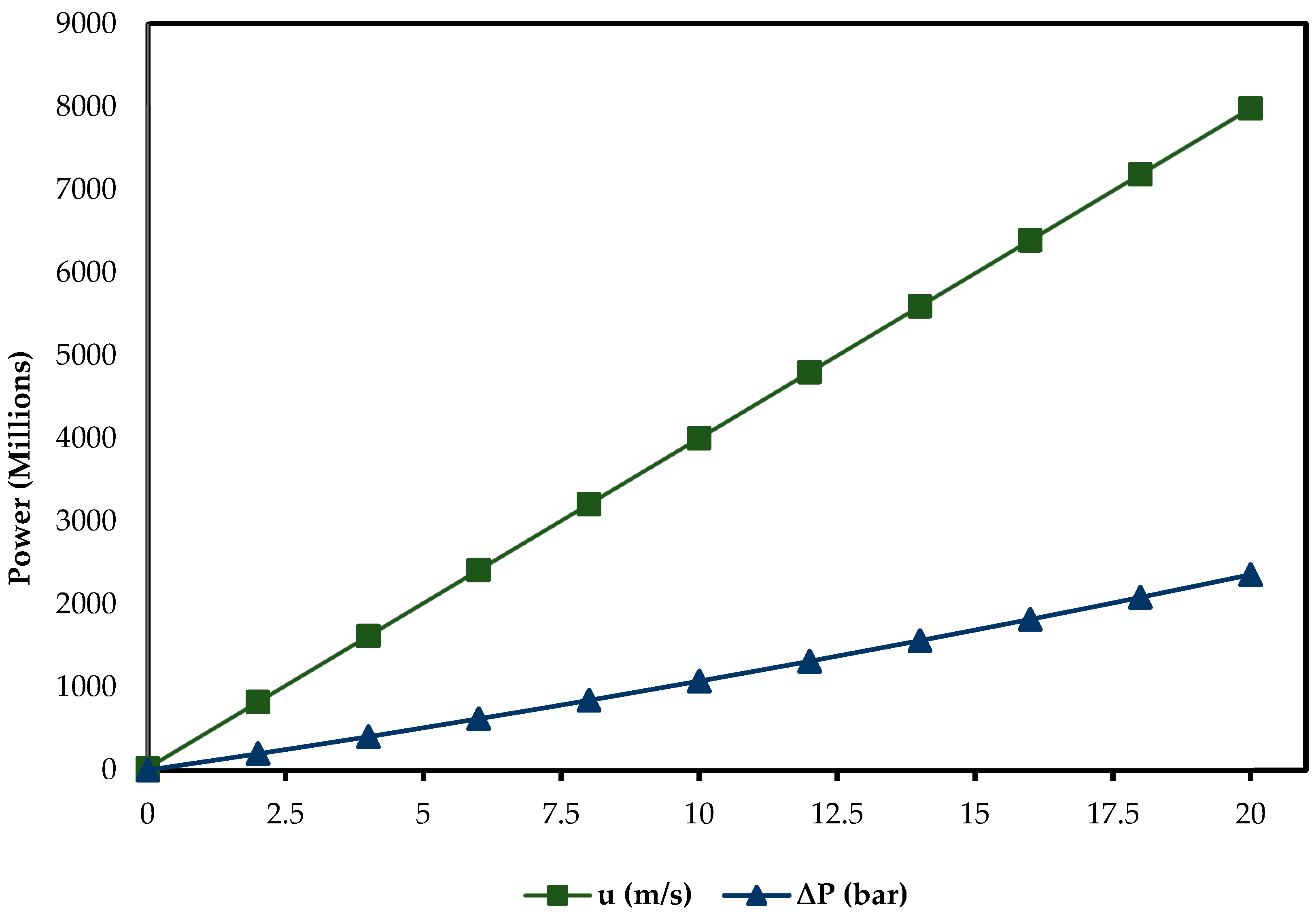
The mathematical models and subsequent simulations have been utilized to investigate the effect of applied pressure difference and water flow velocity on the power requirements of distributing water on a one-kilometer horizontal SDR 13.6 standard polythene water pipe [64]. Figure 11 shows the results of the simulation.
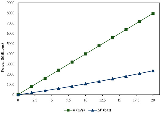
Figure 11.
Results of simulation showing the effect of water velocity and applied pressure on the power requirements.
The SRD polyethylene standard pipes are one of the most used pipes in water distribution networks due to their flexibility, durability and resistance to corrosion, ensuring efficiency, reliability and longevity. The simulation has investigated the energy performance of these pipes under varying operating conditions such as applied pressure difference and flow velocity, providing insights into the design, operation and optimization of water distribution systems.
6. Importance of Mathematical Modelling and Simulation-BasedApproach of the Water–Energy Nexus
6.1. Securing the Future of Hydropower
Climate change has significantly impacted hydropower production through the alteration of precipitation patterns, increasing temperatures and causing more frequent and prolonged droughts [65], reshaping the water availability in many regions. Hydropower plants rely heavily on the water flow consistency of rivers filling up the reservoirs which in recent times have faced increasing variability as the environmental changes disrupt natural hydrological cycles with most of the plants struggling with significant power reduction and even to some extent closing down [66]. The Hoover Dam in the southwestern United States with an annual drying rate of 0.54% [67], the Guri Dam in Venezuela where water is gradually depleting, resulting in rolling blackouts and power rationing in the country [68], the Kariba Dam in Zambia and Zimbabwe, which has had its water recently depleted with the countries experiencing frequent power blackouts [69,70], the Itaipu hydroelectric power plant in Brazil and Uruguay, affected by the disruption of water flow in Paraná River due to droughts [71], and the Three Gorges Dam in China impacted by the Yangtze River Basin’s severe drought [72] are a few examples highlighting the widespread consequences of climate change on hydropower, emphasizing the need for adaptive sophisticated management techniques. Mathematical modeling and simulation of the hydropower water footprint is thus demanded in understanding and mitigating these impacts. Through the integration of reservoir surface area, local climate conditions, such as temperature, humidity, wind speed, and solar radiation, and hydrological patterns, these techniques provide a quantitative basis for the water loss through evaporation and predict future availability of the plants under different climate change scenarios. These valuable insights are important to hydropower operators and policy makes who would use the data to develop strategies to manage water resources more effectively.
6.2. Optimization of Water Consumption and Reducing Damage of Equipment in Geothermal Cooling Systems
In geothermal cooling systems, excessive water and equipment damage due to scaling and corrosion have been a major challenge to plant operators. This problem comes from the need to manage mineral buildup in the system, which results from the continuous water circulation in the cooling towers [73]. When water evaporates it leaves behind dissolved minerals, increasing the concentration of solids which when left unchecked results to mineral deposit scales, which reduces heat transfer and may even clog pipes. Additionally, the accumulation of these minerals, particularly salts, tends to accelerate corrosion which weakens components and increases the risk of system breakdown. To mitigate these issues, operators often resort to blowing down where part of the circulating water is discharged and replaced with fresh make-up water. However frequent blow down, while effective in preventing mineral accumulation in the system, it increases water consumption, making the cooling process costly and environmentally sustainable [74]. One worthwhile strategy to navigate this problem is through optimization of the number of cycles of concentration using mathematical models and simulation. Using these notable tools, plant operators can predict the impact of the various concentration cycles on the water consumption, water chemistry, scaling and corrosion rates and hence find the most efficient number of concentration cycles that minimizes water consumption without compromising equipment longevity. This in turn translates to lower operating costs and reduces the environmental impact while extending equipment life and reducing maintenance needs.
6.3. Achieving the Desired Overall Efficiency at Minimal Energy Consumption in Advanced Oxidation Processes
Optimizing pollutant degradation efficiency in advanced oxidation processes (AOPs) while minimizing energy consumption presents a significant engineering challenge that involves navigating the complex interplay of light intensity, radical generation and contaminant concentration [75]. The chief mechanism in AOPs revolves around the generation of highly reactive species and hydroxyl radicals in the presence of UV radiation which aggressively attacks and oxidizes pollutants to simple non-toxic compounds. The effectiveness of the process hinges on precise control over the distance and orientation of the radiation source relative to the contaminated medium and intensity of the radiation. The radiation intensity that diminishes from the source due to the inverse square law is a fundamental parameter as a too-distant source reduces the radical production while a closer source increases energy consumption without guaranteeing proportional contaminant degradation [53]. Mathematical modeling and simulation offer a pathway to predict and adjust these spatial- and intensity-related factors, enabling optimization of AOP configuration to ensure contaminants are effectively degraded with the least energy input. Through the simulation of these dynamics, plant operators can determine the most ideal operating parameters such as UV lamp placements, optimal distance and angle adjustments, predicting the most effective set-up, thereby minimizing energy consumption while ensuring high pollutant removal.
6.4. Minimizing Energy Consumption in Membrane Separation Processes
The pursuit of sustainable and cost-effective membrane separation systems is strongly intertwined with the reduction in energy consumption of the processes especially in water treatment, wastewater treatment and water desalination [76]. Membrane systems rely on applied pressure gradients and in some processes against osmotic pressure, to drive fluids through a selective permeable membrane which consumes considerable energy. The energy requirement for the process is influenced majorly by the trans-membrane pressure, feed flow rate, solute concentration and membrane properties such as permeability and selectivity. Mathematical modeling and simulation come in handy to help understand and identify optimal operating parameters that minimize energy use, predict energy-intensive conditions, optimize settings and experiment with innovative system designs, ultimately leading to more energy-efficient and sustainable membrane separation technologies [77]. This entails selecting the right computational methods for solving the models and ensuring the mathematical framework is robust enough to be applied across diverse membrane operating conditions, incorporating both mathematical precision and practical insights.
6.5. Paving the Way for Smart Water Distribution Networks
With the aging infrastructure, fluctuating water supply sources, the ever increasing demand and environmental factors such as climate change, water distribution networks face significant challenges in improving their efficiency, reliability and sustainability [78]. Maintaining optimal pressure and flow velocity while minimizing leaks and energy costs is becoming increasingly difficult, often resulting in issues such as frequent pipe bursts, pump failures and water contamination that lead to water disruptions accompanied by costly and time-consuming repairs. Conventional manual monitoring often falls short of providing the responsiveness required for modern water treatment technologies. Mathematical modeling and simulation provide a dynamic and detailed approach to extensively analyze the pressure distribution, water flow and demand patterns allowing the testing of various scenarios such as in the case of equipment failures and peak consumer demands, without disrupting actual operation which helps identify system inefficiencies, predict system responses and refine network’s performance under diverse conditions. Further, the integration of IoT devices with mathematical modeling and simulation has paved the way for smart water distribution networks [79]. Real-time data from IoT sensors provides a continuous update on flow rates and pressure changes that enable simulation to adjust and predict responses in real time. This adaptive water distribution system is not only efficient but also capable of meeting the demands of modern, sustainable water management.
7. Challenges and Prospects
Mathematical modeling and simulation offer a comprehensive framework for examining the intricate dynamics of the water–energy nexus [80]. Despite the numerous advantages associated with these tools, such as improved process efficiency, sustainability and optimum resource utilization, their application is still limited which can be attributed to various factors. Firstly, the complexity of the water–energy nexus makes capturing all its numerous interactions into a mathematical model challenging, computationally expensive and difficult to interpret [81]. Modular and hierarchical modeling should thus be implemented breaking down the water–energy nexus into smaller and more manageable components and leveraging high-performance computing (HPC) and machine learning to handle the complex computation demands. Further, the spatial and temporal variability of the water–energy nexus with both resources fluctuating significantly requires high-resolution data in formulating the models which is often unavailable [82]. Enhanced data collection using remote sensing, IoT devices and other modern technologies and integration of data from multiple sources could immensely improve the data resolution. Additionally, the aging infrastructures, unforeseen breakdowns and human operating errors that disrupt energy production and supply and water treatment and distribution require the incorporation of probabilistic elements, which would make the models so complex limiting further their applicability [83]. To address this, stochastic elements should be incorporated into models to account for uncertainties and probabilistic events to provide an array of possible outcomes and improve robustness of the model. By responding to these challenges, mathematical modeling and simulation have the potential to become even more powerful in navigating the complexities of the water–energy nexus.
8. Conclusions and Future Research Directions
Mathematical modeling and simulation are essential in the water–energy nexus, being indispensable for improving efficiency and sustainability and ensuring optimum resource utilization. The study first provided an in-depth description of the water–energy nexus and a review of the mathematical models and simulation strategies commonly used. A mathematical model and subsequent simulation for the water footprint of hydropower and geothermal renewable energy technologies has been presented considering water consumed through evaporation and cooling respectively. Mathematical modeling and simulation were also applied in determining the energy demands of advanced oxidation processes and membrane separation advanced water treatment. The energy requirements of water distribution have been modeled considering hydrodynamics and accounting for various losses such as frictional drag between the fluid and the pipe walls and the hydraulic transients. The importance of mathematical modeling and simulation to the water–energy nexus has also been extensively discussed. Finally, the paper explores the challenges and prospects of implementing mathematical modeling and simulation to the water–energy nexus. The findings of this study demonstrate mathematical modeling and simulation provide a reliable approach for addressing the complexities of the water–energy nexus, ushering in a new era of sustainability and optimum resource utilization. However, further research is required to realize the full potential of these tools. Future research should focus on the extension of mathematical models and simulation to decentralized renewable energy technologies such as biofuels, green hydrogen fuel cells and solar energy and water treatment technologies such as adsorption, sedimentation and filtration. Additionally, it is necessary to explore the use of frontier new technologies such as machine learning, big data, IoT, digital twin and edge computing to enhance real-time data collection on water and energy consumption, leading to more accurate simulation and predictive capabilities.
Supplementary Materials
The following supporting information can be downloaded at: https://www.mdpi.com/article/10.3390/foundations4040045/s1, Table S1: Hoover Dam hydroelectric power plant data for the month of June 2024; Table S2: High-density polythene (HDPE) standard pipe dimensions.
Author Contributions
M.K.K.; writing—original draft preparation, review and editing, C.A.M.; conceptualization, supervision, review and editing. All authors have read and agreed to the published version of the manuscript.
Funding
This research received no external funding.
Data Availability Statement
All data are available in the manuscript and Supplementary Materials.
Acknowledgments
The authors are grateful to the Renewable Energy, Environment, Nanomaterials and Water (RENWA) Research Group for providing the necessary support in the preparation of this manuscript.
Conflicts of Interest
The authors declare no conflicts of interest.
References
- Helerea, E.; Calin, M.D.; Musuroi, C. Water Energy Nexus and Energy Transition—A Review. Energies 2023, 16, 1879. [Google Scholar] [CrossRef]
- Kiteto, M.; Vidija, B.; Mecha, C.A.; Mrosso, R.; Chollom, M.N. Advances in metal–organic frameworks as adsorbents, photocatalysts and membranes: A new frontier in water purification. Discov. Water 2024, 4, 54. [Google Scholar] [CrossRef]
- Ozili, P.K.; Ozen, E. Global Energy Crisis. In The Impact of Climate Change and Sustainability Standards on the Insurance Market; Sood, K., Grima, S., Young, P., Ozen, E., Balusamy, B., Eds.; Munich Personal RePEc Archive: Munich, Germany, 2023; pp. 439–454. [Google Scholar] [CrossRef]
- Hassan, Q.; Viktor, P.; Al-Musawi, T.J.; Mahmood Ali, B.; Algburi, S.; Alzoubi, H.M.; Khudhair Al-Jiboory, A.; Zuhair Sameen, A.; Salman, H.M.; Jaszczur, M. The renewable energy role in the global energy Transformations. Renew. Energy Focus 2024, 48, 100545. [Google Scholar] [CrossRef]
- Naddaf, M. The world faces a water crisis—4 powerful charts show how. Nature 2023, 615, 774–775. [Google Scholar] [CrossRef] [PubMed]
- Shemer, H.; Wald, S.; Semiat, R. Challenges and Solutions for Global Water Scarcity. Membranes 2023, 13, 612. [Google Scholar] [CrossRef] [PubMed]
- Li, L.; Chen, C.; Li, D.; Breivik, K.; Abbasi, G.; Li, Y.-F. What do we know about the production and release of persistent organic pollutants in the global environment? Environ. Sci. Adv. 2023, 2, 55–68. [Google Scholar] [CrossRef]
- Herrera-Franco, G.; Bollmann, H.A.; Pasqual Lofhagen, J.C.; Bravo-Montero, L.; Carrión-Mero, P. Approach on water-energy-food (WEF) nexus and climate change: A tool in decision-making processes. Environ. Dev. 2023, 46, 100858. [Google Scholar] [CrossRef]
- Lodge, J.W.; Dansie, A.P.; Johnson, F. A review of globally available data sources for modelling the Water-Energy-Food Nexus. Earth-Sci. Rev. 2023, 243, 104485. [Google Scholar] [CrossRef]
- Larsen, M.A.D.; Petrovic, S.; Engström, R.E.; Drews, M.; Liersch, S.; Karlsson, K.B.; Howells, M. Challenges of data availability: Analysing the water-energy nexus in electricity generation. Energy Strategy Rev. 2019, 26, 100426. [Google Scholar] [CrossRef]
- Sun, L.; Cai, Y.; Chen, A.; Zamora, D.; Jaramillo, F. Water footprint and consumption of hydropower from basin-constrained water mass balance. Adv. Water Resour. 2021, 153, 103947. [Google Scholar] [CrossRef]
- Jin, Y.; Behrens, P.; Tukker, A.; Scherer, L. Water use of electricity technologies: A global meta-analysis. Renew. Sustain. Energy Rev. 2019, 115, 109391. [Google Scholar] [CrossRef]
- Lohrmann, A.; Child, M.; Breyer, C. Assessment of the water footprint for the European power sector during the transition towards a 100% renewable energy system. Energy 2021, 233, 121098. [Google Scholar] [CrossRef]
- ESP. How Much Water Do Solar Panels Use vs. Fossil Fuels Energy Solution Providers 2023. Available online: https://energysolutionsolar.com/blog/how-much-water-do-solar-panels-use-vs-fossil-fuels (accessed on 5 November 2024).
- Jia, X.-X.; Klemeš, J.; Tan, R. Overview of Water Use in Renewable Electricity Generation. Huaxue Gongcheng/Chem. Eng. 2021, 89, 403–408. [Google Scholar] [CrossRef]
- Zhu, Y.; Jiang, S.; Zhao, Y.; Li, H.; He, G.; Li, L. Life-cycle-based water footprint assessment of coal-fired power generation in China. J. Clean. Prod. 2020, 254, 120098. [Google Scholar] [CrossRef]
- Statista. Average Water Intensity of Biodiesel and Bioethanol Production Worldwide as of 2024, by Feedstock; Statista Research Department: Hamburg, Germany, 2024; Available online: https://www.statista.com/statistics/1463516/water-footprint-biofuels-worldwide/ (accessed on 5 November 2024).
- Grzegorzek, M.; Wartalska, K.; Kaźmierczak, B. Review of water treatment methods with a focus on energy consumption. Int. Commun. Heat Mass Transf. 2023, 143, 106674. [Google Scholar] [CrossRef]
- Hamawand, I. Energy Consumption in Water/Wastewater Treatment Industry—Optimisation Potentials. Energies 2023, 16, 2433. [Google Scholar] [CrossRef]
- Tow, E.W.; Hartman, A.L.; Jaworowski, A.; Zucker, I.; Kum, S.; AzadiAghdam, M.; Blatchley, E.R.; Achilli, A.; Gu, H.; Urper, G.M.; et al. Modeling the energy consumption of potable water reuse schemes. Water Res. X 2021, 13, 100126. [Google Scholar] [CrossRef]
- Bukhary, S.; Batista, J.; Ahmad, S. An Analysis of Energy Consumption and the Use of Renewables for a Small Drinking Water Treatment Plant. Water 2020, 12, 28. [Google Scholar] [CrossRef]
- Arkhangelsky, E.; Levitsky, I.; Gitis, V. Considering energy efficiency in filtration of engineering nanoparticles. Water Supply 2017, 17, 1212–1218. [Google Scholar] [CrossRef]
- SCEP. Wastewater Infrastructure. Energy.Gov. 2024. Available online: https://www.energy.gov/scep/slsc/wastewater-infrastructure (accessed on 5 November 2024).
- Wang, D.; Junker, A.L.; Sillanpää, M.; Jiang, Y.; Wei, Z. Photo-Based Advanced Oxidation Processes for Zero Pollution: Where Are We Now? Engineering 2023, 23, 19–23. [Google Scholar] [CrossRef]
- Porada, S.; Zhang, L.; Dykstra, J.E. Energy consumption in membrane capacitive deionization and comparison with reverse osmosis. Desalination 2020, 488, 114383. [Google Scholar] [CrossRef]
- Kapur, J.N. Mathematical Modeling; Mercury Learning and Information: Herndon, VA, USA, 2023. [Google Scholar]
- Velten, K.; Schmidt, D.M.; Kahlen, K. Mathematical Modeling and Simulation: Introduction for Scientists and Engineers; Wiley: Hoboken, NJ, USA, 2024. [Google Scholar]
- Elefteriadou, L. Mathematical and Empirical Models; Springer: Berlin/Heidelberg, Germany, 2014; Volume 84, pp. 129–135. [Google Scholar]
- Grafarend, E.W.; Zwanzig, S.; Awange, J.L. Applications of Linear and Nonlinear Models: Fixed Effects, Random Effects, and Total Least Squares; Springer International Publishing: Berlin/Heidelberg, Germany, 2022. [Google Scholar]
- Lou, Z.; Shen, D.; Wang, Y. Two-step principal component analysis for dynamic processes monitoring. Can. J. Chem. Eng. 2017, 96, 160–170. [Google Scholar] [CrossRef]
- Mokhatab, S.; Poe, W.A.; Mak, J.Y. Chapter 19—Process Modeling and Simulation of Gas Processing Plants. In Handbook of Natural Gas Transmission and Processing, 4th ed.; Mokhatab, S., Poe, W.A., Mak, J.Y., Eds.; Gulf Professional Publishing: Houston, TX, USA, 2019; pp. 579–614. [Google Scholar] [CrossRef]
- Loossens, T.; Tuerlinckx, F.; Verdonck, S. A comparison of continuous and discrete time modeling of affective processes in terms of predictive accuracy. Sci. Rep. 2021, 11, 6218. [Google Scholar] [CrossRef] [PubMed]
- Asprion, N.; Böttcher, R.; Höller, J.; Schwartz, P.; Schwientek, J.; Bortz, M. From Single Process Simulation and Optimization to Decision Making Based on a Multitude of Solutions. In Computer Aided Chemical Engineering; Kiss, A.A., Zondervan, E., Lakerveld, R., Özkan, L., Eds.; Elsevier: Amsterdam, The Netherlands, 2019; Volume 46, pp. 7–12. [Google Scholar]
- Garud, S.S.; Mariappan, N.; Karimi, I.A. Two Stage Surrogate Assisted Framework For Box-Constrained Global Optimisation. In Computer Aided Chemical Engineering; Muñoz, S.G., Laird, C.D., Realff, M.J., Eds.; Elsevier: Amsterdam, The Netherlands, 2019; Volume 47, pp. 95–100. [Google Scholar]
- Hasan, M.M.; Rasul, M.G.; Jahirul, M.I.; Khan, M.M.K. Modeling and process simulation of waste macadamia nutshell pyrolysis using Aspen Plus software. Energy Rep. 2022, 8, 429–437. [Google Scholar] [CrossRef]
- Lee, H.H. Finite Element Simulations with ANSYS Workbench 2023: Theory, Applications, Case Studies; SDC Publications: Mission, KS, USA, 2023. [Google Scholar]
- Hadengue, B.; Scheidegger, A.; Morgenroth, E.; Larsen, T.A. Modeling the water-energy nexus in households. Energy Build. 2020, 225, 110262. [Google Scholar] [CrossRef]
- Guerras, L.S.; Martín, M. On the water footprint in power production: Sustainable design of wet cooling towers. Appl. Energy 2020, 263, 114620. [Google Scholar] [CrossRef]
- Killingtveit, Å. 15—Hydroelectric Power. In Future Energy, 3rd ed.; Letcher, T.M., Ed.; Elsevier: Amsterdam, The Netherlands, 2020; pp. 315–330. [Google Scholar] [CrossRef]
- McVeigh, J.C. 12—Alternative energy sources. In Mechanical Engineer’s Reference Book, 12th ed.; Smith, E.H., Ed.; Butterworth-Heinemann: Oxford, UK, 1994; pp. 12-11–12-44. [Google Scholar] [CrossRef]
- Mekonnen, M.; Hoekstra, A. The water footprint of electricity from hydropower. Hydrol. Earth Syst. Sci. 2011, 16, 179–187. [Google Scholar] [CrossRef]
- de Oliveira Bueno, E.; Alves, G.J.; Mello, C.R. Hydroelectricity water footprint in Parana Hydrograph Region, Brazil. Renew. Energy 2020, 162, 596–612. [Google Scholar] [CrossRef]
- Henderson-Sellers, B. Calculating the surface energy balance for lake and reservoir modeling: A review. Rev. Geophys. 1986, 24, 625–649. [Google Scholar] [CrossRef]
- Allen, R.G. Crop Evapotranspiration. FAO Irrig. Drain. Pap. 1998, 56, 60–64. [Google Scholar]
- Archer, R. 20—Geothermal Energy. In Future Energy, 3rd ed.; Letcher, T.M., Ed.; Elsevier: Amsterdam, The Netherlands, 2020; pp. 431–445. [Google Scholar] [CrossRef]
- Huang, W.; Chen, J.; Ma, Q.; Xing, L.; Wang, G.; Cen, J.; Li, Z.; Li, A.; Jiang, F. Developing kilometers-long gravity heat pipe for geothermal energy exploitation. Energy Environ. Sci. 2024, 17, 4508–4518. [Google Scholar] [CrossRef]
- Rutberg, M.J. Modeling Water Use at Thermoelectric Power Plants. Ph.D. Thesis, Massachusetts Institute of Technology, Cambridge, MA, USA, 2012. [Google Scholar]
- Yapıcıoğlu, P.; İrfan, M. Grey water footprint assessment of geothermal water resources in the southeastern Anatolia region. Turk. J. Earth Sci. 2021, 30, 1200–1207. [Google Scholar] [CrossRef]
- Saravanan, A.; Deivayanai, V.C.; Kumar, P.S.; Rangasamy, G.; Hemavathy, R.V.; Harshana, T.; Gayathri, N.; Alagumalai, K. A detailed review on advanced oxidation process in treatment of wastewater: Mechanism, challenges and future outlook. Chemosphere 2022, 308, 136524. [Google Scholar] [CrossRef] [PubMed]
- Mehrjouei, M.; Müller, S.; Möller, D. Energy consumption of three different advanced oxidation methods for water treatment: A cost-effectiveness study. J. Clean. Prod. 2014, 65, 178–183. [Google Scholar] [CrossRef]
- Priyadarshini, M.; Das, I.; Ghangrekar, M.M.; Blaney, L. Advanced oxidation processes: Performance, advantages, and scale-up of emerging technologies. J. Environ. Manag. 2022, 316, 115295. [Google Scholar] [CrossRef] [PubMed]
- Turner, M. Chapter 2—Physics of Cold Plasma. In Cold Plasma in Food and Agriculture; Misra, N.N., Schlüter, O., Cullen, P.J., Eds.; Academic Press: San Diego, CA, USA, 2016; pp. 17–51. [Google Scholar] [CrossRef]
- Voudoukis, N.; Oikonomidis, S. Inverse Square Law for Light and Radiation: A Unifying Educational Approach. Eur. J. Eng. Technol. Res. 2017, 2, 23–27. [Google Scholar] [CrossRef]
- Obotey Ezugbe, E.; Rathilal, S. Membrane Technologies in Wastewater Treatment: A Review. Membranes 2020, 10, 89. [Google Scholar] [CrossRef]
- Castel, C.; Favre, E. Membrane separations and energy efficiency. J. Membr. Sci. 2018, 548, 345–357. [Google Scholar] [CrossRef]
- Mulder, M. Energy Requirements in Membrane Separation Processes. In Membrane Processes in Separation and Purification; Crespo, J.G., Böddeker, K.W., Eds.; Springer: Dordrecht, The Netherlands, 1994; pp. 445–475. [Google Scholar] [CrossRef]
- Wang, Y.; Yok, K.; Wu, W.; Simpson, A.; Weyer, E.; Manzie, C. Minimizing Pumping Energy Cost in Real-Time Operations of Water Distribution Systems Using Economic Model Predictive Control. J. Water Resour. Plan. Manag. 2020, 147, 1–33. [Google Scholar] [CrossRef]
- Karambelkar, S. Hydropower on the Colorado River: Examining Institutions, Conflicts, and Consequences of Changing Dam Operations. Ph.D. Thesis, The University of Arizona, Tucson, AZ, USA, 2020. [Google Scholar]
- Kumar, N.; Arakeri, J.H. A fast method to measure the evaporation rate. J. Hydrol. 2021, 594, 125642. [Google Scholar] [CrossRef]
- Rahmani, K. Reducing water consumption by increasing the cycles of concentration and Considerations of corrosion and scaling in a cooling system. Appl. Therm. Eng. 2017, 114, 849–856. [Google Scholar] [CrossRef]
- Fattahi, A.; Arlos, M.J.; Bragg, L.M.; Liang, R.; Zhou, N.; Servos, M.R. Degradation of natural organic matter using Ag-P25 photocatalyst under continuous and periodic irradiation of 405 and 365 nm UV-LEDs. J. Environ. Chem. Eng. 2021, 9, 104844. [Google Scholar] [CrossRef]
- McKeen, L.W. 4—Markets and Applications for Films, Containers, and Membranes. In Permeability Properties of Plastics and Elastomers, 3rd ed.; McKeen, L.W., Ed.; William Andrew Publishing: Oxford, UK, 2012; pp. 59–75. [Google Scholar] [CrossRef]
- Patel, S.K.; Biesheuvel, P.M.; Elimelech, M. Energy Consumption of Brackish Water Desalination: Identifying the Sweet Spots for Electrodialysis and Reverse Osmosis. ACS EST Eng. 2021, 1, 851–864. [Google Scholar] [CrossRef]
- Alimi, L.; Chaoui, K.; Amirat, A.; Azzouz, S. Study of reliability index for high-density polyethylene based on pipe standard dimension ratio and fracture toughness limits. Int. J. Adv. Manuf. Technol. 2018, 96, 123–136. [Google Scholar] [CrossRef]
- Yasarer, L.M.W.; Sturm, B.S.M. Potential impacts of climate change on reservoir services and management approaches. Lake Reserv. Manag. 2016, 32, 13–26. [Google Scholar] [CrossRef]
- Eslamian, S.; Huda, M.B.; Rather, N.A.; Eslamian, F.A. Handbook of Climate Change Impacts on River Basin Management: Case Studies; CRC Press: Boca Raton, FL, USA, 2024. [Google Scholar]
- Hannoun, D.; Tietjen, T.; Brooks, K. The Influence and Implications of Climate Change on Water Quality in a Large Water Reservoir in the Southwest, USA. Am. J. Clim. Chang. 2022, 11, 197–229. [Google Scholar] [CrossRef]
- Muggah, R.; Brasil, L.; Margolis, M. The climate crisis and displacement in Venezuela. Humanit. Pract. Netw. 2022, 1, 59–62. [Google Scholar]
- Makombe, E.K.; Chanza, N. The State, Climate Change and Energy Transition in Zimbabwe, 1992–2022. Glob. Environ. 2024, 17, 546–578. [Google Scholar] [CrossRef]
- Dube, K.; Nhamo, G. Evaluating climate Change’s impact on hydroelectricity in the Zambezi river basin. Heliyon 2023, 9, e23235. [Google Scholar] [CrossRef] [PubMed]
- Gwynn, M.A. International law and transboundary dams: Lessons learned from the Binational Entity ITAIPU (Brazil and Paraguay). Front. Clim. 2023, 5, 1272254. [Google Scholar] [CrossRef]
- Ma, M.; Qu, Y.; Lyu, J.; Zhang, X.; Su, Z.; Gao, H.; Yang, X.; Chen, X.; Jiang, T.; Zhang, J.; et al. The 2022 extreme drought in the Yangtze River Basin: Characteristics, causes and response strategies. River 2022, 1, 162–171. [Google Scholar] [CrossRef]
- Gautier, A.; Wetter, M.; Sulzer, M. Resilient cooling through geothermal district energy system. Appl. Energy 2022, 325, 119880. [Google Scholar] [CrossRef]
- Müller, S.I.; Chapanova, G.; Diekow, T.; Kaiser, C.; Hamelink, L.; Hitsov, I.P.; Wyseure, L.; Moed, D.H.; Palmowski, L.; Wintgens, T. Comparison of cooling tower blowdown and enhanced make up water treatment to minimize cooling water footprint. J. Environ. Manag. 2024, 367, 121949. [Google Scholar] [CrossRef] [PubMed]
- Senobari, S.; Nezamzadeh-Ejhieh, A. A novel ternary nano-composite with a high photocatalyitic activity: Characterization, effect of calcination temperature and designing the experiments. J. Photochem. Photobiol. A Chem. 2020, 394, 112455. [Google Scholar] [CrossRef]
- Chen, T.; Wei, X.; Chen, Z.; Morin, D.; Alvarez, S.V.; Yoon, Y.; Huang, Y. Designing energy-efficient separation membranes: Knowledge from nature for a sustainable future. Adv. Membr. 2022, 2, 100031. [Google Scholar] [CrossRef]
- Kancherla, R.; Nazia, S.; Kalyani, S.; Sridhar, S. Modeling and simulation for design and analysis of membrane-based separation processes. Comput. Chem. Eng. 2021, 148, 107258. [Google Scholar] [CrossRef]
- Ramos, H.M.; Carravetta, A.; Nabola, A.M. New Challenges in Water Systems. Water 2020, 12, 2340. [Google Scholar] [CrossRef]
- Quadar, N.; Chehri, A.; Jeon, G.; Ahmad, A. Smart Water Distribution System Based on IoT Networks, a Critical Review; Springer: Singapore, 2021; pp. 293–303. [Google Scholar]
- Shammi, M.; Mostafizur, M.R. 13—Desalination technologies and potential mathematical modeling for sustainable water–energy nexus. In Water Engineering Modeling and Mathematic Tools; Samui, P., Bonakdari, H., Deo, R., Eds.; Elsevier: Amsterdam, The Netherlands, 2021; pp. 251–269. [Google Scholar] [CrossRef]
- Siakwah, P.; Torto, O. Analysis of the Complexities in the Water-Energy-Food Nexus: Ghana’s Bui Dam Experience. Front. Sustain. Food Syst. 2022, 6, 734675. [Google Scholar] [CrossRef]
- Wang, S.; Yang, R.; Shi, S.; Wang, A.; Liu, T.; Yang, J. Characteristics and Influencing Factors of the Spatial and Temporal Variability of the Coupled Water–Energy–Food Nexus in the Yellow River Basin in Henan Province. Sustainability 2023, 15, 13977. [Google Scholar] [CrossRef]
- Huang, Y.; Zhang, J.; Ren, Z.; Xiang, W.; Sifat, I.; Zhang, W.; Zhu, J.; Li, B. Next generation decentralized water systems: A water-energy-infrastructure-human nexus (WEIHN) approach. Environ. Sci. Water Res. Technol. 2023, 9, 2446–2471. [Google Scholar] [CrossRef]


Disclaimer/Publisher’s Note: The statements, opinions and data contained in all publications are solely those of the individual author(s) and contributor(s) and not of MDPI and/or the editor(s). MDPI and/or the editor(s) disclaim responsibility for any injury to people or property resulting from any ideas, methods, instructions or products referred to in the content. |
© 2024 by the authors. Licensee MDPI, Basel, Switzerland. This article is an open access article distributed under the terms and conditions of the Creative Commons Attribution (CC BY) license (https://creativecommons.org/licenses/by/4.0/).