Maximum Entropy Solutions with Hyperbolic Cosine and Secant Distributions: Theory and Applications

Abstract

This work explores the hyperbolic cosine and hyperbolic secant functions within the framework of the maximum entropy principle, deriving these probability distribution functions from first principles. The resulting maximum entropy solutions are applied to various physical systems, including the repulsive oscillator and solitary wave solutions of the advection equation, using the method of moments. Additionally, a different moment analysis using experimental and theoretical inputs is employed to address non-linear systems described by the non-linear Schrödinger equation, non-linear diffusion equation, and Korteweg–de Vries equation, demonstrating the versatility of this approach. These findings demonstrate the broad applicability of maximum entropy methods in solving different differential equations, with potential implications for future research in non-linear dynamics and transport physics.

1. Introduction

The hyperbolic cosine and its inverse, the hyperbolic secant, probability density functions are often overlooked distribution functions, even though they describe a broad range of diverse phenomena. The hyperbolic cosine distribution has been applied to describe the wave functions of atomic and molecular systems [1], model cerebral emboli to test Doppler signal detection [2], characterize the infinitesimal drift in diffusion processes described by the Fokker–Planck equation [3], and assess and model responses to questionnaires in psychological and sociological studies [4]. The hyperbolic secant probability distribution function has been applied to studying the similarity of twine, $2\times 2$ contingency tables [5], and the interplay of imitation and innovation in modeling economic growth [6] and population growth [7]. In general, hyperbolic functions have had applications in computational physics [8], data analysis [9], and machine learning [10].

The unit hyperbola is given as the right-hand branch of $x^2-y^2=1$, where the Cartesian coordinates $(x,y)$ can be described by $(coshu,sinhu)$, where the hyperbolic cosine function is defined as the mean of the exponential function and its reciprocal,

$$coshu={\displaystyle \frac{e^u+e^{-u}}{2}}$$

(1)

and the hyperbolic sine is defined as the residual mean of the exponential and its reciprocal,

$$sinhu={\displaystyle \frac{e^u-e^{-u}}{2}}.$$

(2)

It is worth mentioning that u can be interpreted as an imaginary angle, thus relating the hyperbolic trigonometry functions to the familiar circular trigonometry functions.

As the hyperbolic cosine and secant functions are of specific importance in this work, their relation is given explicitly as follows:

$$sechu={cosh}^{-1}u={\displaystyle \frac{2}{e^u+e^{-u}}}.$$

(3)

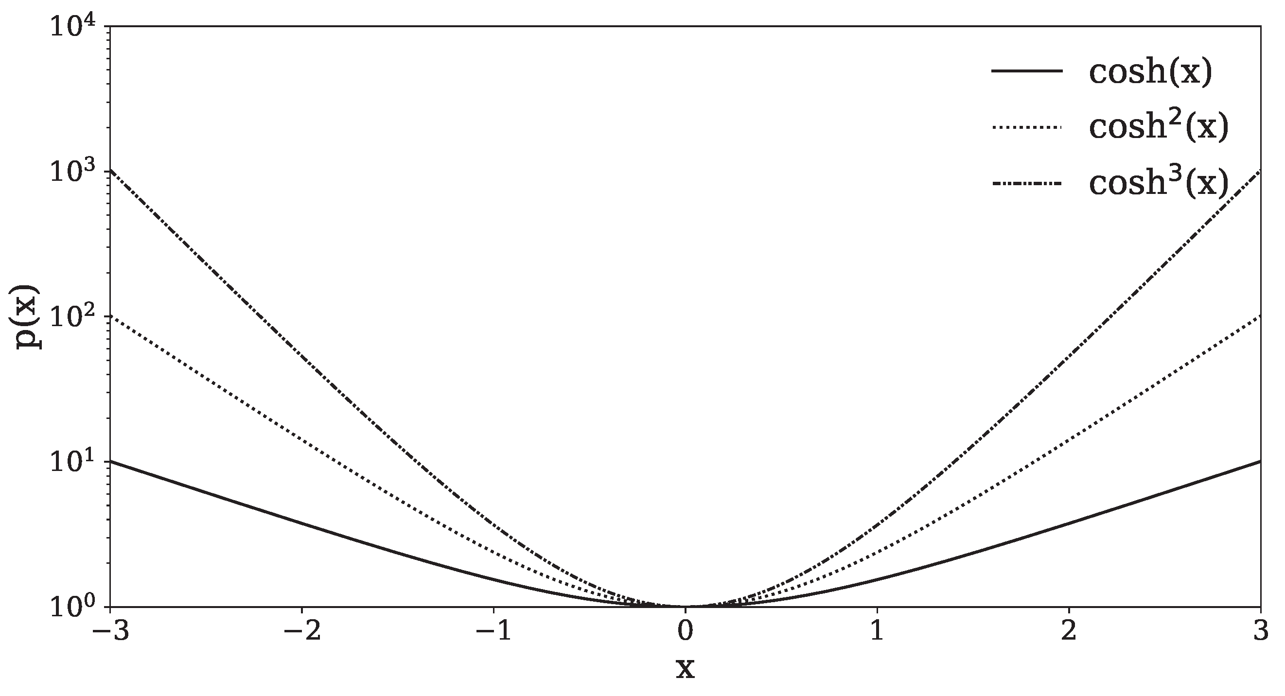
2. Properties of the Hyperbolic Cosine Probability Function

The hyperbolic cosine probability distribution function [11] is a symmetric distribution function (see Figure 1) given that it is bounded on a symmetric interval.

The hyperbolic secant probability distribution function [12,13] is a symmetric distribution function (see Figure 2) reminiscent of the Gaussian distribution. Note that the Gaussian distribution is described by two statistical moments, the mean and variance. In contrast, the hyperbolic secant distribution is described by three statistical moments, the mean, the variance, and the kurtosis. The standard continuous hyperbolic probability distribution function is given as follows:

$$p\left(x\right)={\displaystyle \frac{1}{2}}{\displaystyle \frac{1}{cosh\left(\pi \frac{x}{2}\right)}}={\displaystyle \frac{1}{2}}sech\left(\pi {\displaystyle \frac{x}{2}}\right)$$

(4)

where the unit variance is centered around zero and whose domain is given by $-\infty$ to $+\infty$. This distribution may be further generalized [12] to the following:

$$p\left(x\right)={\displaystyle \frac{1}{2\sigma }}{\displaystyle \frac{1}{cosh\left(\pi \frac{x-\mu }{2\sigma }\right)}}={\displaystyle \frac{1}{2\sigma }}sech\left(\pi {\displaystyle \frac{x-\mu }{2\sigma }}\right)$$

(5)

where $\sigma$ describes the scaling of the variance and $\mu$ describes of the offset of the distribution.

3. The Maximum Entropy Principle

Entropy and probability are intimately related to one another. Shannon defines the information entropy [14] expression for a continuous distribution dependent on a random variable, x, as follows:

$$S(x)=-\int p(x)lnp(x)dx$$

(6)

where $S\left(x\right)$ is the entropy and $p\left(x\right)$ is the probability distribution function. The Maximum Entropy Principle states the entropy should be maximized within the confines of the known constraints [15]. This is the natural extension of Laplace’s Principle of Insufficient Reason, which states that one should assign equal probabilities to event outcomes unless some data or evidence is present.

Typically, the constraints of the probability distribution functions are described by the ith moment $m_i$,

$$m_i=\int x^{i}p\left(x\right)dx$$

(7)

where $x^i$ is the ith power of the random variable. Recall that the zeroth moment is simply the normalization, the first moment is the average, the second moment is related to the width, and so forth in the probability distribution function $p\left(x\right)$.

Another avenue for constraints on the probability distribution is to examine constraints of a similar but slightly different form,

$$\langle f(x)\rangle =\int f(x)p(x)dx$$

(8)

where $f\left(x\right)$ is some continuous function within the examined interval. An example of such a constraint would be found in [16], where the potential energy was used to constrain the probability distribution function due to the presence of an external conservative force.

4. Derivation of the Hyperbolic Cosine Probability Distribution Function from the Maximum Entropy Principle

In order to derive the probability distribution using the MaxEnt technique, constraints must be specified. Total probabilities will be normalized. It is worth mentioning that total probability is not required to be normalized to one, although typically they are. This first constraint is realized as the zeroth moment of the distribution,

$$m_0=\langle 1\rangle =\int p\left(x\right)dx.$$

(9)

The second constraint under consideration is conjectured to be the moment with respect to the natural logarithm of the hyperbolic cosine function,

$$\zeta =\langle ln(coshx)\rangle =\int ln(coshx)p(x)dx.$$

(10)

The Lagrange undetermined multipliers, ${\lambda }_0$ and ${\lambda }_{\zeta }$, are applied to the constraints of the normalization and average of the natural logarithm of the hyperbolic cosine, respectively, and are used to constrain the Shannon information entropy,

$$S\left(x\right)=-\int p\left(x\right)lnp\left(x\right)dx-{\lambda }_0\left(\int p\left(x\right)dx-m_0\right)-{\lambda }_{\zeta }\left(\int ln(coshx)p(x)dx-\zeta \right).$$

(11)

The derivative operator is applied with respect to the probability of the entropy and is set equal to zero to determine the maximum probability distribution associated with these constraints,

$$\delta S=0=-\int \left[1+lnp\left(x\right)+{\lambda }_0+{\lambda }_{\zeta }ln(coshx)\right]dx.$$

(12)

The constant terms can be grouped into a single term, ${\lambda }_0^{\prime }$, defined as, ${\lambda }_0^{\prime }=1+{\lambda }_0$. It is important to point out that oftentimes it is fashionable and facilitates a deeper understanding of this parameter to rewrite the constant term in terms of a natural logarithm reminiscent of the partition function from statistical physics. Rewriting the maximum entropy equation in terms of this new term leads to the following:

$$\delta S=0=-\int \left[{\lambda }_0^{\prime }+lnp\left(x\right)+{\lambda }_{\zeta }ln(coshx)\right]dx.$$

(13)

The integrand must equal zero for this equation to always equal zero in a nontrivial manner. Isolating the probability distribution function,

$$lnp\left(x\right)=-{\lambda }_0^{\prime }-{\lambda }_{\zeta }ln(coshx),$$

(14)

and exponentiating both sides of the equation to solve for the probability distribution function leads to the following result:

$$p\left(x\right)=e^{-{\lambda }_0^{\prime }}{cosh}^{-{\lambda }_{\zeta }}\left(x\right).$$

(15)

Several transformations may be employed at this stage so as to further generalize the solution. This probability distribution function is centered on zero. The distribution could be centered about some other point, $x_0$, and there could be a scaling, $\sigma$, associated with this distribution, so the transformation $x\to {\displaystyle \frac{x-x_0}{\sigma }}$ could be applied, along with the fact that $e^{-{\lambda }_0^{\prime }}$ is simply a constant and could be renamed, yet again, as $K^{\prime }=e^{-{\lambda }_0^{\prime }}$, and rewriting the Lagrange multiplier $-{\lambda }_{\zeta }$ as ${\gamma }^{\prime }$ allows for the maximum entropy distribution to be rewritten as follows:

$$p\left(x\right)=K^{\prime }{cosh}^{{\gamma }^{\prime }}\left({\displaystyle \frac{x-x_0}{\sigma }}\right),$$

(16)

where now all that is left to perform is to determine the unknown parameters tied to the Lagrange multipliers $K^{\prime }$ and ${\gamma }^{\prime }$. This can be rewritten as follows:

$$p\left(x\right)=K{\mathrm{sech}}^{\gamma }\left({\displaystyle \frac{x-x_0}{\sigma }}\right)$$

(17)

where $\gamma =-{\gamma }^{\prime }$ and the normalization K must be recalculated in order to ensure that the probability distribution function is properly normalized.

5. Applications of the Maximum Entropy Technique with Hyperbolic Cosine and Secant Distributions

In this section, the MaxEnt results of Section 4 are applied in several ways to various physical phenomena. First, there is a comparison between the recent results of the probability distribution function and the MaxEnt solution for the catenary given in Section 5.1. Then, the MaxEnt solution is applied using the method of moments to determine the solutions to the repulsive oscillator and to solitary waves described by the advection equation in Section 5.2 and Section 5.3. In Section 5.4, Section 5.5 and Section 5.6, it is assumed that the moments can be determined experimentally and by applying the MaxEnt solutions to determine the theoretical moments of the probability distribution functions of the non-linear Schrödinger equation, the non-linear diffusion equation, and the non-linear Korteweg–de Vries equation.

5.1. Catenary

An immediate application of the found MaxEnt hyperbolic cosine probability distribution is that of a uniform flexible chain/wire/rope that is fixed at its ends and hangs under its own weight due to a uniform gravitational field. In reference [17], it was found, using a different method, that the probability distribution function associated with the catenary is as follows:

$$p\left(x\right)={cosh}^{-2}\left({\displaystyle \frac{x-x_0}{\sigma }}\right).$$

(18)

The reasoning follows that the curve of a catenary is well known, and determining an infinitesimal length can be found. From this, the probability distribution function can easily be reconstructed. It is easily seen that Equation (18) follows from the derived MaxEnt probability distribution determined in Equation (16).

5.2. Repulsive Oscillator

The repulsive harmonic oscillator [18], also known as the modified oscillator or simply as the linear repulsive force, has many applications. The linear repulsive force appears in the theory of vibrations with damped and driven oscillator systems described by the Duffy equation [19]. Often, a linear repulsive force term can be found in the Langevin equation used by the Fokker–Planck equation [20]. Many classical systems, such as the inverted pendulum, have been studied under the influence of a repulsive linear force. Linear repulsive forces have been studied extensively in the context of quantum mechanics, and studies of solutions of solitons under the influence of a repulsive potential have been studied [21]. The quantum mechanical linear oscillator and linear anharmonic oscillator have been studied extensively [22].

The repulsive harmonic oscillator is modeled by the second-order differential equation of the form,

$${\displaystyle \frac{d^{2}p\left(x\right)}{d{x}^2}}=k^{2}p\left(x\right)$$

(19)

where $p\left(x\right)$ is the probability distribution function and k is a constant related to the strength of the potential.

The boundary condition for Equation (19) is as follows:

$$p(x\to \infty )=a.$$

(20)

This constraint is needed in order to truncate the unbounded nature of the hyperbolic cosine PDF and the normalization requirement. In real-world applications, such truncations are frequently required due to constraints inherent in equipment capabilities, instrumentation accuracy, budget restrictions, or physiological limits [23,24,25,26].

It is assumed that the solution takes the form of the MaxEnt solution with ${\gamma }^{\prime }=1$, $p\left(x\right)=K^{\prime }cosh\left({\sigma }_{2}x\right)$ on physical grounds where ${\sigma }_2={\displaystyle \frac{1}{\sigma }}$. In order to use the methods of moments, both sides of Equation (19) are multiplied by $x^2$ and integrated over the space,

$${\int }_0^a{x}^2{\displaystyle \frac{d^{2}p\left(x\right)}{d{x}^2}}dx=k^2{\int }_0^a{x}^{2}p\left(x\right)dx.$$

(21)

Noting that the right-hand side is the second moment and performing the integration by parts of the left-hand side yields the following:

$$x^2{\displaystyle \frac{\partial p\left(x\right)}{\partial x}}{|}_0^a-{\int }_0^a{\displaystyle \frac{\partial p\left(x\right)}{\partial x}}2xdx=k^2\langle x^2\rangle .$$

(22)

Integrating by parts the integral on the right-hand sides leads to the following:

$$x^2{\displaystyle \frac{\partial p\left(x\right)}{\partial x}}{|}_0^a-2\left[xp\left(x\right){|}_0^a-{\int }_0^{a}p\left(x\right)dx\right]=k^2\langle x^2\rangle .$$

(23)

This leads to the following equation,

$$x^2{\displaystyle \frac{\partial p\left(x\right)}{\partial x}}{|}_0^a-2\left[xp\left(x\right){|}_0^a-\langle 1\rangle \right]=k^2\langle x^2\rangle$$

(24)

Using the MaxEnt solution, $p\left(x\right)=K^{\prime }cosh\left({\sigma }_{2}x\right)$, the first moment can be determined as follows:

$$\begin{array}{cc}\hfill \langle 1\rangle & ={\int }_0^{a}p\left(x\right)dy={\int }_0^a{K}^{\prime }cosh\left({\sigma }_{2}x\right)dx\hfill \end{array}$$

(25)

$$\begin{array}{cc}\hfill & =K^{\prime }{\displaystyle \frac{sinh\left({\sigma }_{2}x\right)}{{\sigma }_2}}{|}_0^a\hfill \end{array}$$

(26)

$$\begin{array}{cc}\hfill & =K^{\prime }{\displaystyle \frac{sinh\left({\sigma }_{2}a\right)}{c_2}}\hfill \end{array}$$

(27)

as well as the second moment,

$$\begin{array}{cc}\hfill \langle x^2\rangle & ={\int }_0^a{x}^{2}p\left(x\right)dx={\int }_0^{a}K{x}^{2}cosh\left({\sigma }_{2}x\right)dx\hfill \end{array}$$

(28)

$$\begin{array}{cc}\hfill & =K^{\prime }{\displaystyle \frac{({\sigma }_2^2{x}^2+2)sinh{\sigma }_{2}x-2{\sigma }_{2}xcosh{\sigma }_{2}x}{{\sigma }_2^3}}{|}_0^a\hfill \end{array}$$

(29)

$$\begin{array}{cc}\hfill & =K^{\prime }{\displaystyle \frac{({\sigma }_2^2{a}^2+2)sinh{\sigma }_{2}a-2{\sigma }_{2}acosh{\sigma }_{2}a}{{\sigma }_2^3}}\hfill \end{array}$$

(30)

which then can be used in Equation (24). Applying the limits of integration and performing the algebra results in determining ${\sigma }_2=\pm k$ and choosing the positive root, the result that ${\sigma }_2=k$. Applying the result of the ${\sigma }_2$ constant to Equation (27) results in determining the normalization constant $K^{\prime }={\displaystyle \frac{k}{sinhka}}$. The situation where $k=1$ and $a=3$ is plotted in Figure 3.

5.3. Advection Equation

The one-dimensional advection equation [27,28,29] governs the transport of a scalar field. In this context, the scalar field represents the PDF $p(x,t)$, which is being advected by a constant velocity v and is expressed as follows:

$${\displaystyle \frac{\partial p(x,t)}{\partial t}}+v{\displaystyle \frac{\partial p(x,t)}{\partial x}}=0.$$

(31)

This equation has a wide range of applications, such as modeling the propagation of waves in shallow channels, traffic flow, and pollution transport in the atmosphere. A particular solution to the advection equation is the solitary wave, also known as the soliton solution, which takes the following form:

$$p(x,t)={\displaystyle \frac{1}{2}}{\mathrm{sech}}^2(x-vt).$$

(32)

These solutions are remarkable, since they retain the same localized shape for all time, t. We can determine the solution using the MaxEnt solution Equation (17),

$$p(x,t)=K{\mathrm{sech}}^2({\sigma }_{2}x-{\sigma }_1)$$

(33)

where we have assumed $\gamma =2$ and have rewritten ${\sigma }_2=1/a$ and ${\sigma }_1=x_0/a$.

Rearranging the advection Equation (31),

$${\displaystyle \frac{\partial p(x,t)}{\partial t}}=-v{\displaystyle \frac{\partial p(x,t)}{\partial x}}$$

(34)

and spatially integrating both sides over x yields the following:

$${\int }_{-\infty }^{\infty }{\displaystyle \frac{\partial p(x,t)}{\partial t}}dx=-{\int }_{-\infty }^{\infty }v{\displaystyle \frac{\partial p(x,t)}{\partial x}}dx.$$

(35)

Assuming that the derivative operator can be removed from under the spatial integral along with the constant velocity,

$${\displaystyle \frac{d}{dt}}{\int }_{-\infty }^{\infty }p(x,t)dx=-v{\int }_{-\infty }^{\infty }{\displaystyle \frac{\partial p(x,t)}{\partial x}}dx,$$

(36)

it is noted that the integral on the left is the zeroth moment, the normalization, and that the integral on the right yields zero due to the boundary conditions imposed on the probability distribution function. This yields the following:

$${\displaystyle \frac{d\langle 1\rangle }{dt}}=0$$

(37)

which is the statement that the zeroth moment, i.e., the normalization, is a constant (usually taken to be one),

$$\langle 1\rangle =1.$$

(38)

Again, applying the same idea to Equation (34), but this time multiplying both sides by x and integrating the following:

$${\int }_{-\infty }^{\infty }{\displaystyle \frac{\partial p(x,t)}{\partial t}}xdx=-{\int }_{-\infty }^{\infty }v{\displaystyle \frac{\partial p(x,t)}{\partial x}}xdx,$$

(39)

assuming that the temporal derivative operator can be removed from the integral on the left and integrating-by-parts on the right yields the following:

$${\displaystyle \frac{d}{dt}}{\int }_{-\infty }^{\infty }p(x,t)xdx=-v\left[{xp(x,t)|}_{-\infty }^{\infty }-{\int }_{-\infty }^{\infty }p(x,t)dx\right],$$

(40)

where the surface goes to zero due to the boundary conditions imposed on the probability distribution function, $p(x,t)$, the integral on the right-hand side is identified with the first spatial moment, $\langle x\rangle$, and the remaining integral on the right is identified with the zeroth moment, the normalization $\langle 1\rangle$. Note that the differential equations for the moments are a closed set. Finally, this results in the following:

$${\displaystyle \frac{d\langle x\rangle }{dt}}=v.$$

(41)

This is integrated to determine the temporal dependence of the first moment,

$$\langle x\rangle =vt$$

(42)

where the constant of integration is set to zero due to the initial conditions.

Examining the second moment using Equation (34), but this time multiplying both sides by $x^2$ and integrating the following:

$${\int }_{-\infty }^{\infty }{\displaystyle \frac{\partial p(x,t)}{\partial t}}{x}^{2}dx=-{\int }_{-\infty }^{\infty }v{\displaystyle \frac{\partial p(x,t)}{\partial x}}{x}^{2}dx,$$

(43)

assuming that the temporal derivative operator can be removed from the integral on the left and integrating-by-parts on the right yields the following:

$${\displaystyle \frac{d}{dt}}{\int }_{-\infty }^{\infty }p(x,t)x^{2}dx=-v\left[x^2{p(x,t)|}_{-\infty }^{\infty }-2{\int }_{-\infty }^{\infty }xp(x,t)dx\right],$$

(44)

where the surface term vanishes due to the boundary conditions as $x\to \pm \infty$. Noting the integral on the left-hand side is the second moment and the integral on the right-hand side is the first moment results in the following:

$${\displaystyle \frac{d\langle x^2\rangle }{dt}}=2v\langle x\rangle .$$

(45)

Integrating leads to determining the second moment as follows:

$$\langle x^2\rangle =2v^2{t}^2+C^{\prime }$$

(46)

where $C^{\prime }$ is the unknown constant of integration that must be kept, since there are no known initial conditions to apply here.

In order to determine the moments from the MaxEnt solution, the following relation [30] will be useful:

$$\int x^n{\mathrm{sech}}^2(x-t)dx=2{(-i\pi )}^n{B}_n\left({\displaystyle \frac{1}{2}}+i{\displaystyle \frac{t}{\pi }}\right)$$

(47)

where $B_n\left(z\right)$ are the Bernoulli polynomials. The zeroth moment is found to be the following:

$$\langle 1\rangle ={\int }_{-\infty }^{\infty }p(x,t)dx={\int }_{-\infty }^{\infty }K{\mathrm{sech}}^2({\sigma }_{2}x-{\sigma }_1)dx=K{\displaystyle \frac{2}{{\sigma }_2}},$$

(48)

whereas the first moment is determined to be the following:

$$\langle x\rangle ={\int }_{-\infty }^{\infty }xp(x,t)dx={\int }_{-\infty }^{\infty }xK{\mathrm{sech}}^2({\sigma }_{2}x-{\sigma }_1)dx=K{\displaystyle \frac{2{\sigma }_1}{{\sigma }_2^2}},$$

(49)

and the second moment is calculated to be the following:

$$\langle x^2\rangle ={\int }_{-\infty }^{\infty }{x}^{2}p(x,t)dx={\int }_{-\infty }^{\infty }{x}^{2}K{\mathrm{sech}}^2({\sigma }_{2}x-{\sigma }_1)dx={\displaystyle \frac{K}{{\sigma }_2^3}}\left(2{\sigma }_1^2+{\displaystyle \frac{{\pi }^2}{3}}\right).$$

(50)

Equating the zeroth moments, Equations (38) and (48) leads to the following:

$$K={\displaystyle \frac{{\sigma }_2}{2}}.$$

(51)

Equating the first moments, Equations (42) and (49), and using the normalization result, Equation (51) leads to the following:

$${\displaystyle \frac{{\sigma }_1}{{\sigma }_2}}=vt.$$

(52)

Equating the second moments, Equations (46) and (50), and using the normalization result, Equation (51) leads to the following:

$${\displaystyle \frac{{\pi }^2}{6{\sigma }_2}}=C^{\prime }.$$

(53)

The variance is examined to determine the integration constant, $C^{\prime }$. Solitary waves change position, but not shape; thus, the variance will be a constant. The variance is determined to be the following:

$$\begin{array}{ccc}\hfill \mathrm{var}\left(x\right)& =& \langle x^2\rangle -{\langle x\rangle }^2\hfill \end{array}$$

(54)

$$\begin{array}{ccc}& =& \left({\left(vt\right)}^2+{\displaystyle \frac{{\pi }^2}{6{\sigma }_2^2}}\right)-{\left(vt{\sigma }_2\right)}^2.\hfill \end{array}$$

(55)

The position of the solitary wave is given as $vt$, which changes with time, but the variance must remain constant for a solitary wave; thus, for the time-dependent first and third terms on the right-hand side of Equation (54) to cancel, this implies the following:

$${\sigma }_2=1.$$

(56)

Substituting the result of Equation (56) into Equation (52) leads to the following:

$${\sigma }_1=vt.$$

(57)

Likewise, substituting Equation (56) into Equation (51) results in the following:

$$K={\displaystyle \frac{1}{2}}.$$

(58)

Taking these results and substituting them into the MaxEnt solution (33) results in the well-known solution given in Equation (32).

5.4. Non-Linear Schrödinger Equation

A different approach is employed here to solve the non-linear Schrödinger equation. Since the general form of the MaxEnt solution is known, it is possible to solve the differential equation without explicitly knowing the equation itself. One can directly determine the solution by assuming the MaxEnt form and experimentally measuring the moments of the distribution.

The one-dimensional stationary Schrödinger-type equation [31,32,33,34] with a cubic non-linearity term is given as follows:

$$-{\displaystyle \frac{1}{2}}{\displaystyle \frac{d^2}{d{x}^2}}p\left(x\right)-2k{\left[p\left(x\right)\right]}^3+{\displaystyle \frac{1}{2}}{k}^{2}p\left(x\right)=0$$

(59)

where the solution is expressed as follows:

$$p\left(x\right)=\sqrt{{\displaystyle \frac{k}{2}}}\mathrm{sech}\left(kx\right).$$

(60)

This equation has been applied to modeling plasma physics [35], light propagation in nonlinear optical media such as in optical fibers [36], and modeling dilute Bose–Einstein condensates [37].

It is interesting to note that the differential equation does not need to be solved explicitly if one can experimentally determine the moments of the solution.

The zeroth moment (which is experimentally determined, but here the actual distribution is used for the example calculation), is given as follows:

$$\langle 1\rangle ={\int }_{-\infty }^{\infty }p\left(x\right)dx={\displaystyle \frac{\pi }{\sqrt{2k}}}$$

(61)

using the MaxEnt solution of the following form,

$$p\left(x\right)=K\mathrm{sech}\left({\sigma }_{2}x\right)$$

(62)

where $\gamma =1$, and the ${\sigma }_1$ term ignored for the stationary solution symmetric about the origin, to determine the first moment, is determined to be the following:

$$\langle 1\rangle ={\int }_{-\infty }^{\infty }p\left(x\right)dx={\int }_{-\infty }^{\infty }K\mathrm{sech}\left({\sigma }_{2}x\right)dx={\displaystyle \frac{K\pi }{{\sigma }_2}}.$$

(63)

The first moment, determined experimentally, is given as follows:

$$\langle x\rangle ={\int }_{-\infty }^{\infty }xp\left(x\right)dx=0$$

(64)

and the second moment, again determined experimentally, is found to be as follows:

$$\langle x^2\rangle ={\int }_{-\infty }^{\infty }{x}^{2}p\left(x\right)dx={\displaystyle \frac{{\pi }^3}{4\sqrt{2}{k}^{\frac{5}{2}}}}$$

(65)

which the MaxEnt solution is to determine the second moment,

$$\langle x^2\rangle ={\int }_{-\infty }^{\infty }{x}^{2}p\left(x\right)dx={\int }_{-\infty }^{\infty }{x}^{2}K\mathrm{sech}\left({\sigma }_{2}x\right)dx={\displaystyle \frac{K{\pi }^3}{4{\sigma }_2^3}}.$$

(66)

Using the experimentally determined moments and theoretically calculated moments using the MaxEnt results in the unknown values of amplitude and coefficient in the argument of the hyperbolic trig function. Equating Equations (61) and (63) results in the following:

$$K={\displaystyle \frac{{\sigma }_2}{\sqrt{2k}}}$$

(67)

and equating Equations (65) and (66) yields the following:

$${\displaystyle \frac{K}{{\sigma }_2^3}}={\displaystyle \frac{1}{\sqrt{\pi k^5}}}$$

(68)

Substituting the normalization constant, Equation (67), written in terms of ${\sigma }_2$ into the Equation (68) and solving for ${\sigma }_2$, yields the following:

$${\sigma }_2=k$$

(69)

and using this result in Equation (67) results in the following:

$$K={\displaystyle \frac{k}{\sqrt{2k}}}$$

(70)

which results in the solution given in Equation (60).

5.5. Non-Linear Diffusion

Consider the stationary non-linear diffusion equation [38,39] in one dimension,

$$D{\displaystyle \frac{{\partial }^{2}p\left(x\right)}{\partial x^2}}={\lambda }_{1}p\left(x\right)-{\lambda }_{2}p{\left(x\right)}^2$$

(71)

where the D is the diffusion constant and ${\lambda }_1$, and ${\lambda }_2$ are both positive constants that describe the linear and nonlinear source and sink terms. The solution to this differential equation is as follows:

$$p\left(x\right)={\displaystyle \frac{3{\lambda }_1}{2{\lambda }_2}}{\mathrm{sech}}^2\left(\sqrt{{\displaystyle \frac{{\lambda }_1}{4D}}}\right).$$

(72)

Employing the same strategy as performed in Section 5.4 to experimentally determine the moments and then to determine theoretically the moments from the MaxEnt solution that will once again be assumed to be of the form, $p\left(x\right)=K{\mathrm{sech}}^2\left({\sigma }_{2}x\right)$.

The zeroth moment, which would be determined experimentally, is given as

$$\langle 1\rangle ={\int }_{-\infty }^{\infty }p\left(x\right)dx={\displaystyle \frac{24D}{{\lambda }_2}}$$

(73)

using the MaxEnt solution to determine the zeroth moment, is determined to be as follows:

$$\langle 1\rangle ={\int }_{-\infty }^{\infty }p\left(x\right)dx={\int }_{-\infty }^{\infty }K{\mathrm{sech}}^2\left({\sigma }_{2}x\right)dx={\displaystyle \frac{K2}{{\sigma }_2}}.$$

(74)

The first moment, determined experimentally, is given as follows:

$$\langle x\rangle ={\int }_{-\infty }^{\infty }xp\left(x\right)dx=0$$

(75)

and the second moment, again determined experimentally, is found to be the following:

$$\langle x^2\rangle ={\int }_{-\infty }^{\infty }{x}^{2}p\left(x\right)dx={\displaystyle \frac{32D^3{\pi }^2}{{\lambda }_1^2{\lambda }_2}}$$

(76)

which the MaxEnt solution is to determine the second moment,

$$\langle x^2\rangle ={\int }_{-\infty }^{\infty }{x}^{2}p\left(x\right)dx={\int }_{-\infty }^{\infty }{x}^{2}K{\mathrm{sech}}^2\left({\sigma }_{2}x\right)dx={\displaystyle \frac{K{\pi }^2}{6{\sigma }_2^3}}.$$

(77)

Using the experimentally determined moments and theoretically calculated moments using the MaxEnt results in the unknown values of normalization and coefficient in the argument of the hyperbolic trig function. Equating Equations (73) and (74) results in the following:

$$K={\displaystyle \frac{12D}{{\lambda }_2}}{\sigma }_2$$

(78)

and equating Equations (76) and (77) and applying Equation (78) yields the following:

$${\sigma }_2={\displaystyle \frac{{\lambda }_1}{4D}}$$

(79)

Inserting this result into Equation (78) yields the value of the normalization constant K,

$$K={\displaystyle \frac{3{\lambda }_1}{{\lambda }_2}}$$

(80)

and using this result in Equation (67) results in the solution given in Equation (72).

5.6. Korteweg–de Vries Equation

The non-dimensional Korteweg–de Vries equation is a non-linear third-order partial differential equation [40],

$${\displaystyle \frac{\partial p(x,t)}{\partial t}}=6p(x,t){\displaystyle \frac{\partial p(x,t)}{\partial x}}-{\displaystyle \frac{{\partial }^{3}p(x,t)}{\partial x^3}}$$

(81)

where $p(x,t)$ describes a wave surface at position x at time t. One of the simplest solutions of Equation (81) is the solitary transverse wave solution, known as a soliton that has the form of a hyperbolic secant square nature,

$${\mathrm{sech}}^2\left(x\right).$$

(82)

These solutions describe a myriad of non-linear dispersive wave propagation phenomena in media such as shallow waves in a canal [41], charged particles moving through a plasma producing solitary waves that cause pitting in the space shuttle windows [42], and oscillations of hyper-deformed nuclei described in non-linear liquid-drop models from nuclear physics [43].

A thought-provoking application of the MaxEnt solution to Equation (81) is to assume the solution of the equation and then to experimentally determine the parameters of the solution from experimental observations. This was described by one of the authors in Ref. [16]. An example of this program carried out with the Korteweg–de Vries soliton is described. A total of 10,000 random numbers from the logistic distribution were generated for a soliton of two arbitrary spatial units at five arbitrary temporal units. Gaussian noise was added to the signal and then fitted for the parameters of the MaxEnt solution in the form of Equation (17). The resulting fits from both the ideal and noisy signal distributions are shown in Figure 4.

6. Discussion and Results

The hyperbolic cosine and hyperbolic secant probability distribution functions were derived from the principle of maximum entropy for the first time using a novel constraint. These distributions were then applied across a wide array of applications to demonstrate their practical utility. The hyperbolic cosine probability distribution function was explored in relation to the well-known catenary problem, while the method of moments was employed to determine the unknown parameters associated with the truncated hyperbolic cosine probability distribution as applied to the repulsive harmonic oscillator. Further application of the method of moments was applied to the advection equation in order to determine the unknown parameters of the ${\mathrm{sech}}^2$ distribution solution.

In order to determine the unknown parameters associated with the the probability distribution functions for non-linear differential equations, a different strategy was employed. The play-off between experiment and theory was used to determine the unknown parameters for the sech probability distribution function associated with the non-linear Schrödinger equation. The same approach was used for the ${\mathrm{sech}}^2$ probability distribution function associated with the non-linear diffusion equation. Again, the same technique was employed to determine the unknown parameters associated with the hyperbolic secant function for the non-linear Korteweg–de Vries Equation, except this time, the experimental data were generated via a simulation in order to demonstrate how this novel technique would be applied in a real-world scenario.

This work encompasses several limitations that warrant further exploration. While the standard moment constraints in the maximum entropy technique are given well-defined physical interpretations, the physical significance of the hyperbolic cosine moment constraint remains unclear, beyond its ability to accurately reproduce the appropriate probability distribution function. Additionally, the analyses presented here assume prior knowledge of the power of the probability distribution functions. These limitations highlight areas for continued research to enhance the depth and applicability of these findings.

This study opens several avenues for future research and potential applications across a broad spectrum of physical systems. The methodologies and insights gained from exploring the hyperbolic cosine and secant probability distribution functions under the maximum entropy principle can be adapted and applied to other complex systems.

The Korteweg–de Vries equation along with the modified Korteweg–de Vries equation is rich in study and application of MaxEnt techniques. A variety of situations can be further explored, such as the addition of various non-linearity terms along with varying initial and different boundary conditions.

The Boussinesq and Boussinesq-type equations [44,45] describe weakly non-linear waves with small amplitudes and relatively long wavelengths. These equations accept solitary wave and soliton-type solutions where there is a balance between the dispersive effects of the medium and non-linear effects. The primary contexts that this equation is applied to modeling are shallow surface water waves such as modeling tsunami waves, groundwater hydrology with the flow of groundwater over sloping bedrock in hillslope areas [46], and ocean engineering to predict wave propagation along shallow coastline areas [47]. This is an area of active research that the MaxEnt technique could be applied to in the future.

Another application of this work is the study of heat transfer associated with the heating or cooling of fins due to convective processes. Investigations into solutions of the Camassa–Holm equation [48] that have soliton-like solutions are suggested.

A particularly intriguing avenue for future research is exploring the intersection of this work with the deformed statistical framework developed by Kaniadakis [49,50], which is based on special relativity, which in turn is based upon the hyperbolic trigonometric functions. Investigating the connections between this fractal entropy-based statistics and the methods discussed here could lead to a deeper understanding of the underlying physics of these complex systems.

7. Conclusions

In this work, the hyperbolic functions are reviewed. The properties of hyperbolic cosine and secant functions as probability distribution functions and their applications are outlined. The Maximum Entropy Principle is discussed at length, and common constraints involving moment equations are highlighted and subsequently used in a derivation of the hyperbolic cosine and secant probability distributions. These solutions are then applied by utilizing the method of moments to several physical systems, both stationary and dynamic, such as the repulsive oscillator and solitary waves described by the advection equation. A different approach utilizing both the experimentally measured as well as theoretically determined moments, solutions to physical systems, both stationary and dynamic, described by the non-linear Schrödinger equation, non-linear diffusion equation, and the Korteweg–de Vries equation are found.

References

1. Sahin, E.; Ozdogan, T.; Orbay, M. On the effectiveness of exponential type orbitals with hyperbolic cosine functions in atomic calculations. J. Math. Chem. 2017, 55, 1849–1856. [Google Scholar] [CrossRef]
2. Kouamé, D.; Biard, M.; Girault, J.; Bleuzen, A.; Tranquart, F.; Patat, F. Statistical and Neuro-fuzzy approaches for emboli detection. In Proceedings of the 2004 12th European Signal Processing Conference, Vienna, Austria, 6–10 September.
3. Barndorff-Nielsen, O. Hyperbolic Distributions and Distributions on Hyperbolae. Scand. J. Stat. 1978, 5, 151–157. [Google Scholar]
4. Andrich, D.; Luo, G. A hyperbolic cosine latent trait model for unfolding dichotomous single-stimulus responses. Appl. Psychol. Meas. 1993, 17, 253–276. [Google Scholar] [CrossRef]
5. Ding, P. Three Occurrences of the Hyperbolic-Secant Distribution. Am. Stat. 2014, 68, 32–35. [Google Scholar] [CrossRef]
6. Gallay, O.; Hashemi, F.; Hongler, M.-O. Imitation, proximity, and growth a collective swarm dynamics approach. Adv. Complex Syst. 2019, 22, 1–43. [Google Scholar] [CrossRef]
7. Parand, K.; Abbasbandy, S.; Kazem, S.; Rad, J.A. A novel application of radial basis functions for solving a model of first-order integro-ordinary differential equation. Commun. Nonlinear Sci. Numer. Simul. 2011, 16, 4250–4258. [Google Scholar] [CrossRef]
8. Mao, X.; Joshi, V.; Jaiman, R. A variational interface-preserving and conservative phase-field method for the surface tension effect in two-phase flows. arXiv 2020, arXiv:2007.15887. [Google Scholar] [CrossRef]
9. Haluszczynski, A.; Aumeier, J.; Herteux, J.; Räth, C. Reducing network size and improving prediction stability of reservoir computing. Chaos Interdiscip. J. Nonlinear Sci. 2020, 30, 063136. [Google Scholar] [CrossRef]
10. Ngom, M.; Marin, O. Approximating periodic functions and solving differential equations using a novel type of Fourier Neural Networks. arXiv 2020, arXiv:2005.13100. [Google Scholar]
11. András, S.; Baricz, Á. Properties of the probability density function of the non-central chi-squared distribution. J. Math. Anal. Appl. 2008, 346, 395–402. [Google Scholar] [CrossRef]
12. Fischer, M.J. Generalized Hyperbolic Secant Distributions: With Applications to Finance, 1st ed.; Springer: New York, NY, USA, 2013. [Google Scholar]
13. Harkness, W.L.; Harkness, M.L. Generalized hyperbolic secant distributions. J. Am. Stat. Assoc. 1968, 63, 329–337. [Google Scholar] [CrossRef]
14. Shannon, C.E. A Mathematical Theory of Communication. Bell Syst. Tech. J. 1948, 27, 379–423. [Google Scholar] [CrossRef]
15. Jaynes, E.T. Information Theory and Statistical Mechanics. Phys. Rev. 1957, 106, 620–630. [Google Scholar] [CrossRef]
16. Secrest, J.A.; Conroy, J.M.; Miller, H.G. A unified view of transport equations. Physica A 2020, 547, 124403. [Google Scholar] [CrossRef]
17. Guseo, R. Diffusion of innovations dynamics, biological growth and catenary function. Physica A 2016, 464, 1–10. [Google Scholar] [CrossRef]
18. Wintner, A. On Linear Repulsive Forces. Am. J. Math. 1949, 71, 362–366. [Google Scholar] [CrossRef]
19. Taylor, J. Analysis of the Nonlinear vibrations of electrostatically actuated Micro-controlled in Harmonic Detection of Resonance. Ph.D. Dissertation, Clemon University, Clemson, SC, USA, 2008. [Google Scholar]
20. Risken, H. Fokker-Planck Equation. In The Fokker-Planck Equation; Springer Series in Synergetics; Springer: Berlin/Heidelberg, Germany, 1996; Volume 18. [Google Scholar]
21. Stoychev, K.T.; Primatarowa, M.T.; Kamburova, R.S. Resonant interaction of solitons with extended defects. J. Optoelectron. Adv. Mater. 2007, 9, 155–158. [Google Scholar]
22. Villegas-Martínez, B.M.; Moya-Cessa, H.M.; Soto-Eguibar, F. Exact and approximated solutions for the harmonic and anharmonic repulsive oscillators: Matrix method. Eur. Phys. J. D 2020, 74, 137. [Google Scholar] [CrossRef]
23. Tokmachev, M.S. Modeling of truncated probability distributions. IOP Conf. Ser. Mater. Sci. Eng. 2018, 441, 012056. [Google Scholar] [CrossRef]
24. Zybin, K.P.; Sirota, V.A.; Ilyin, A.S. Structure functions of fully developed hydrodynamic turbulence: An analytical approach. Phys. Rev. E 2010, 82, 056324. [Google Scholar] [CrossRef]
25. Gómez-Liévano, A.; Vysotsky, V.; Lobo, J. Artificial increasing returns to scale and the problem of sampling from lognormals. Environ. Plan. B Urban Anal. City Sci. 2021, 48, 1574–1590. [Google Scholar] [CrossRef]
26. Kamiński, M. Stochastic boundary element method analysis of the interface defects in composite materials. Compos. St. ruct. 2012, 94, 394–402. [Google Scholar] [CrossRef]
27. Hereman, W. Shallow Water Waves and Solitary Waves. In Solitons; Helal, M.A., Ed.; Encyclopedia of Complexity and Systems Science Series; Springer: New York, NY, USA, 2022. [Google Scholar]
28. Riecke, H. Solitary waves under the influence of a long-wave mode. Phys. D Nonlinear Phenom. 1996, 92, 69–94. [Google Scholar] [CrossRef]
29. Sen, A.; Ahalpara, D.P.; Thyagaraja, A.; Krishnaswami, G.S. A KdV-like advection–dispersion equation with some remarkable properties. Commun. Nonlinear Sci. Numer. Simul. 2012, 17, 4115–4124. [Google Scholar] [CrossRef]
30. Boyadzhiev, K.N. A note on Bernoulli polynomials and solitons. J. Nonlinear Math. Phys. 2007, 14, 174–178. [Google Scholar] [CrossRef]
31. Gürses, M.; Pekcan, A. Nonlocal nonlinear Schrödinger equations and their soliton solutions. J. Math. Phys. 2018, 59, 051501. [Google Scholar] [CrossRef]
32. Seadawy, A.R. Approximation solutions of derivative nonlinear Schrödinger equation with computational applications by variational method. Eur. Phys. J. Plus 2015, 130, 182. [Google Scholar] [CrossRef]
33. Hayashi, N.; Ozawa, T. On the derivative nonlinear Schrödinger equation. Phys. D Nonlinear Phenom. 1992, 55, 14–36. [Google Scholar] [CrossRef]
34. Ma, W.; Chen, M. Direct search for exact solutions to the nonlinear Schrödinger equation. Appl. Math. Comput. 2009, 215, 2835–2842. [Google Scholar] [CrossRef]
35. Taha, T.R.; Ablowitz, M.J. Analytical and numerical aspects of certain nonlinear evolution equations. II. Numerical, nonlinear Schrödinger equation. J. Comput. Phys. 1984, 55, 203–230. [Google Scholar] [CrossRef]
36. Stephanovich, V.A.; Olchawa, W.; Kirichenko, E.V.; Dugaev, V.K. 1D solitons in cubic-quintic fractional nonlinear Schrödinger model. Sci. Rep. 2022, 12, 15031. [Google Scholar] [CrossRef] [PubMed]
37. Carr, L.D.; Kutz, J.N.; Reinhardt, W.P. Stability of stationary states in the cubic nonlinear Schrödinger equation: Applications to the Bose-Einstein condensate. Phys. Rev. E 2001, 63, 066604. [Google Scholar] [CrossRef] [PubMed]
38. Ulmer, W. Solution spectrum of nonlinear diffusion equations. Int. J. Theor. Phys. 1992, 31, 1549–1567. [Google Scholar] [CrossRef]
39. Aibinu, M.O.; Thakur, S.C.; Moyo, S. Exact solutions of nonlinear delay reaction–diffusion equations with variable coefficients. Partial. Differ. Equations Appl. Math. 2021, 4, 100170. [Google Scholar] [CrossRef]
40. Fokas, A.S. The Korteweg-de Vries equation and beyond. Acta Appl. Math. 1995, 39, 295–305. [Google Scholar] [CrossRef]
41. Korteweg, D.J.; de Vries, G. On the Change of Form of Long Waves Advancing in a Rectangular Canal, and on a New Type of Long Stationary Waves. Phil. Mag. 1895, 39, 422–443. [Google Scholar] [CrossRef]
42. Truitt, A.S.; Hartzell, C.M. Simulating Plasma Solitons from Orbital Debris Using the Forced Korteweg–de Vries Equation. J. Spacecr. Rocket. 2020, 57, 876–897. [Google Scholar] [CrossRef]
43. Ludu, A.; Draayer, J.P. Nonlinear Modes of Liquid Drops as Solitary Waves. Phys. Rev. Lett. 1998, 80, 2125. [Google Scholar] [CrossRef]
44. Darvishi, M.T.; Najafi, M.; Wazwaz, A.M. Soliton solutions for Boussinesq-like equations with spatio-temporal dispersion. Ocean. Eng. 2017, 130, 228–240. [Google Scholar] [CrossRef]
45. Todorov, M.D. Nonlinear Waves: Two-Dimensional Boussinesq Equation. Boussinesq Paradigm and Soliton Solutions; Morgan & Claypool Publishers: San Rafael, CA, USA, 2018; pp. 1–33. [Google Scholar]
46. Nadeem, M.; Islam, A.; Şenol, M.; Alsayaad, Y. The dynamical perspective of soliton solutions, bifurcation, chaotic and sensitivity analysis to the (3+ 1)-dimensional Boussinesq model. Sci. Rep. 2024, 14, 9173. [Google Scholar] [CrossRef] [PubMed]
47. Vivas-Cortez, M.; Arshed, S.; Perveen, Z.; Sadaf, M.; Akram, G.; Rehan, K.; Saeed, K. Analysis of perturbed Boussinesq equation via novel integrating schemes. PLoS ONE 2024, 19, e0302784. [Google Scholar] [CrossRef] [PubMed]
48. Gottwald, G.A. Dispersive regularizations and numerical discretizations for the inviscid Burgers equation. J. Phys. A Math. Theor. 2007, 40, 14745. [Google Scholar] [CrossRef]
49. Kaniadakis, G. Statistical mechanics in the context of special relativity. Phys. Rev. E 2002, 66, 056125. [Google Scholar] [CrossRef] [PubMed]
50. Kaniadakis, G. Statistical mechanics in the context of special relativity. II. Phys. Rev. E 2005, 72, 036108. [Google Scholar] [CrossRef]
Figure 1. The above figure represents various non-normalized hyperbolic cosine functions raised to different powers. Note the logarithmic scale of the y-axis. This family of curves demonstrates the characteristics of the function along the x-axis for 3 x 3 .
Foundations 04 00046 g001
Figure 2. The above figure represents various non-normalized inverse hyperbolic cosine (inverse secant) functions raised to various powers. This family of curves demonstrates the characteristics of the function in general as x ± , as well as the width of the distribution.
Foundations 04 00046 g002
Figure 3. Probability distribution function, p ( x ) , for the repulsive oscillator as a function of some variable, x, initially sitting at an unstable equilibrium point at zero. The value of k was chosen to be 1 inverse unit, while the extreme position value of a was chosen to be three units for illustrative purposes.
Foundations 04 00046 g003
Figure 4. The above left is a simulated soliton solution to the Korteweg–de Vries for a pulse with a width of 2 units located at time t = 5 units along with the fit parameters. The plot on the right is the same pulse, but with Gaussian noise added to the signal. This illustrates experimentally fitting for the MaxEnt solution.
Foundations 04 00046 g004
Disclaimer/Publisher’s Note: The statements, opinions and data contained in all publications are solely those of the individual author(s) and contributor(s) and not of MDPI and/or the editor(s). MDPI and/or the editor(s) disclaim responsibility for any injury to people or property resulting from any ideas, methods, instructions or products referred to in the content.