Article

Fundamental Spacetime Representations of Quantum Antenna Systems

1
Zhejiang University/University of Illinois at Urbana-Champaign Institute (the ZJU-UIUC Institute), Zhejiang University, 718 East Haizhou Road, Haining 314400, China
2
Electrical and Computer Engineering Department, University of Illinois at Urbana-Champaign, Engineering Hall MC 266, 1308 West Green Street, Champaign, IL 61820, USA
Foundations 2022, 2(1), 251-289; https://doi.org/10.3390/foundations2010019
Submission received: 15 November 2021 / Revised: 26 January 2022 / Accepted: 3 February 2022 / Published: 2 March 2022
(This article belongs to the Special Issue Advances in Fundamental Physics)

Abstract

:
We utilize relativistic quantum mechanics to develop general quantum field-theoretic foundations suitable for understanding, analyzing, and designing generic quantum antennas for potential use in secure quantum communication systems and other applications. Quantum antennas are approached here as abstract source systems capable of producing what we dub “quantum radiation.” We work from within a generic relativistic framework, whereby the quantum antenna system is modeled in terms of a fundamental quantum spacetime field. After developing a framework explaining how quantum radiation can be understood using the methods of perturbative relativistic quantum field theory (QFT), we investigate in depth the problem of quantum radiation by a controlled abstract source functions. We illustrate the theory in the case of the neutral Klein-Gordon linear quantum antenna, outlining general methods for the construction of the Green’s function of a source—receiver quantum antenna system, the latter being useful for the computation of various candidate angular quantum radiation directivity and gain patterns analogous to the corresponding concepts in classical antenna theory. We anticipate that the proposed formalism may be extended to deal with a large spectrum of other possible controlled emission types for quantum communications applications, including, for example, the production of scalar, fermionic, and bosonic particles, where each could be massless or massive. Therefore, our goal is to extend the idea of antenna beyond electromagnetic waves, where now our proposed QFT-based concept of a quantum antenna system could be used to explore scenarios of controlled radiation of any type of relativistic particles, i.e., effectively transcending the well-known case of photonic systems through the deployment of novel non-standard quantum information transmission carriers such as massive photons, spin- 1 / 2 particles, gravitons, antiparticles, higher spin particles, and so on.

1. Introduction

The main objective of this paper is to develop conceptual, physical, and mathematical foundations for quantum antenna theory based on a very broad approach to generic quantum fields produced and consumed by source and sink systems separated in spacetime. Quantum antenna technology is a recent emerging subfield within the larger and more fluid research area often referred to as quantum engineering, quantum technologies, or just quantum information processing. In particular, and within this subfield, we find that the main intention behind the desire for developing a new “quantum antenna technology” is to serve the needs of current and future quantum communication systems [1,2,3,4], where information is transmitted using quantum states [5,6], regardless of whether digital data are encoded as classical bits or qbits [1,7,8,9,10], with obvious applications to physical-layer security [11,12,13,14]. However, the peculiar system known as “the quantum antenna” may also perform functions other than mere information transmission in wireless quantum links, for example, quantum tomography, quantum state estimation, biophotonics, sensing, molecular communications, space exploration, and other applications [13,15,16,17,18,19,20,21,22,23,24,25,26].
We believe that quantum antenna theory and technology may be viewed as an attempt to synthesize three already established subfields: (1) classical antennas [27,28], (2) optical nanoantennas [29,30], and (3) quantum emitters [29,31]. As such, a quantum antenna is often confused with one of these three topics. For example, occasionally, laser sources or photodiodes are treated as quantum antennas by some authors working in free space optical communications. This is not what we understand by the term here. A laser source could constitute a part of the q-antenna system, while a larger part, for example a terahertz or an optical antenna [29,32], may serve as a secondary reflector as in nanoantennas [30]. In addition, an atom emitting a photon after undergoing a transition from excited to ground states is not considered an “antenna” in this paper. Instead, we propose the following general definition:
Definition 1 (Antennas).
By the term antenna, we follow classical antenna theory where the antenna system is defined as an externally controlled spatiotemporal current distribution capable of controlling the spatiotemporal properties of the radiation emitted by the antenna system.
It will be seen that the most salient point in this definition is the emphasis on the following three features:
  • The source is a controllable current distribution function of both space and time.
  • Ultimately, the source current is externally controlled.
  • A spatiotemporal current distribution profile serving as a model for a quantum antenna source can control the radiation proprieties in both space and time, and usually for near- and far-field scenarios as well.
Hence, the existence of spatiotemporal, externally controlled source current distributions capable of modifying its produced radiation in both space and time is the main content of antenna theory.
Clearly enough, mainstream examples in quantum optics such as a laser source by itself, or an isolated atom undergoing a spontaneous emission of light, do not fall under a conceptual umbrella such as the one supplied by Definition 1, at least not naturally. However, such conventional quantum optical sources may still serve as essential sub-components of such systems. For example, probably, the most natural method to inject a controlled time signal into a radiating nanostructure is through a modulated laser beam. However, controlling the spatial distribution of the radiating current excited by this time signal would require the use of additional methods and objects; for instance, an optical antenna, or an engineered metamaterial, or an optimized array of point sources. Even though the data to be transmitted are encoded into time signals, in general, the quantum antenna system is much more complex than its time excitation method. There is a need, then, to understand the complex and multifaceted nature of the spatiotemporal structure of the radiation field emitted by a generic quantum system at a very broad level. This paper is a contribution toward this goal.
The classical theory of controlled radiation has been extensively studied and developed in applied electromagnetics [27,28,33,34,35]. On the other hand, the general theory of quantum antennas has not been investigated in depth so far, in spite of the publication in recent years of a number of reports and proposals about the subject, not restricted only to quantum wireless communications but also involving other topics as well, e.g., see [15,16,17,18,19,20,21]. Some of the main conceptual and philosophical hurdles that a viable theory of quantum antennas need to overcome include, though by no means are restricted to, the following issues:
  • Understanding what is meant by quantum radiation.
  • Understanding the role played by particle emission dynamics in light of the wave-particle duality characteristic of quantum phenomena.
  • Understanding the complex role played by quantum fields, propagators, and Green’s functions in quantum radiation.
  • Understanding the role played by many-particle states/interactions in quantum radiation processes.
It should be noted that these conceptual and technical issues are still considered difficult open research fields in both foundational and applied research as they have not been resolved even within standard quantum field theory itself. For instance, it is still not clear what the ultimate meaning of “particle” in quantum fields is [36,37]; questions about the nature of quantum excitations in interacting field theories have been asked in the past [38] and are still being investigated up to date [39]. Therefore, there is a need to re-examine the subject of quantum antennas at a very general and fundamental level, that of developing possible foundations for the topic that may help illuminate current and future open theoretical problems on one hand, and to help devise and evolve new genera of quantum systems and applications on the other hand. A viable candidate for such foundational approach, we believe, is to formulate the entire problem of quantum antennas and quantum radiation using a relativistic spacetime formalism (QFT in this case).
Our intended goals in the present article include a wide spectrum. Most of these objectives are research related and can be classified as part of the emerging area of quantum antenna theory within both quantum physics and quantum engineering. Yet, additionally, other aspects in our work are pedagogical, relating to the wish to reach a wide multidisciplinary audience. We summarize these two flavors of our main goals as follows:
  • Primary research objectives of the present article:
    • Generalizing the concept of antennas beyond acoustic and electromagnetic antennas, the two concepts that have dominated the field so far, by demonstrating how relativistic QFT can be used to formulate a single and unified concept of “quantum radiators” valid for a large number of possible radiation processes in nature.
    • Providing a concrete illustration of some of the potential algorithmic capabilities of the spacetime formalism of quantum antennas by constructing various possible candidates for radiation pattern functions and gains in the case of the quantum (spin-0) Klein–Gordon q-antennas.
  • Secondary (pedagogical) objectives of the present article:
    • Introducing new applications of fundamental theory (here relativistic quantum mechanics) to different audiences, e.g., quantum engineering and quantum technology research.
    • Introducing the subject of QFT in a self-sufficient manner by providing detailed appendices explaining how relativistic quantum mechanics is formulated for an audience familiar only with nonrelativistic quantum mechanics.1
This paper is organized as follows. In Section 2, the classical theory of antennas is re-examined, and the comparison with the new, more general concept of quantum source radiators is explored at the thematic level in order to prep the reader for the subsequent, more technical quantum-field theoretic treatment. This is followed in Section 3 by a very broad view on the theory of quantum radiators developed based on interacting quantum mechanics, without much emphasis at this stage on the relativistic quantum field theoretic scenario. The purpose is to map out the generic structure of the problem and to highlight the distinction between linear and nonlinear quantum antennas. Starting from Section 4, we narrow down our focus to the special but rich enough special case of the neutral Klein–Gordon field linear quantum antenna, which appears to exhibit many of the salient features of the general quantum antenna system. Then, the abstract formal and physical structure of such a system is explicated in Section 5. To provide more concrete applications of the theory, Section 6 presents a series of examples and constructions aiming at illustrating how one may define radiation pattern measures such as directivity and gain (transmission) coefficients in quantum antenna systems. Finally, we end up with conclusions.

2. Antenna Theory: Classical and Quantum Radiation Scenarios

In analogy to classical antenna theory [27,35,40], we formally define a quantum antenna in terms of the mathematical representation of a radiating source term as follows:
Definition 2 (Quantum Antennas).
Within the context of relativistic quantum field theory, a quantum antenna (q-antenna) J is an operator map of the form
J : J Ψ ,
where Ψ is a quantum field system produced by the abstract source function
J : M 4 K ,
which maps the Minkowski spacetime M 4 of special relativity to the set K = R (real numbers) or K = C (complex numbers). We assume that the function J ( x ) , x D s M 4 is integrable over any spacetime region D s of interest. We further assume that the source J ( x ) is compactly supported; i.e., c l { D s } is compact where cl is the closure operator in the standard Euclidean topology on R 4 .
Physically, the main property of the q-antenna (source) function J ( x ) is that it controls the quantum radiation Ψ ( x ) , x M 4 , emitted by the source system J ( x ) , x D s M 4 . The generic configuration itself is shown in Figure 1. In fact, much of this paper will concentrate on understanding the precise nature of how a generic source function J ( x ) can control the spacetime structure of the quantum field emission Ψ ( x ) in applications characteristic of the special context of an arbitrary quantum communication system (source-channel-detector system). Thus, the article’s main scope is the theoretical foundations of the physical layer of the quantum communication link structure, e.g., how a quantum state can be directed to a given spacetime region through the choice of a proper abstract source function. The particular discipline devoted to this problem is the area we dub quantum antenna theory, which is a relatively new interdisciplinary research area.
Remark 1. 
It may be noted here that there is a similarity between the quantum communication problem [7] and the quantum measurement problem in quantum physics [41,42,43]. The analogy is manifested by the common underlying abstract structure shared by the two distinct processes of communications and generalized quantum measurement [1,8]. Both involve a source of information (often called quantum state preparation in QM), which is localized within a given spacetime region; and a process of destructive consumption of the transmitted information, this time localized at a receiver or detector located at a timelike-distant spacetime region [43,44]. The quantum receiver system’s ultimate objective is to extract the maximum amount of information embodied in the received quantum state in QM, or quantum field in QFT, through the judicious utilization of optimized combinations of measurement operations and signal processing algorithms.
Quantum antenna systems turn out to be considerably more complex to understand and analyze than conventional antennas, where the latter antenna type is often approached within the framework based on classical electromagnetism (and sometimes acoustics). A reason behind this noticeable difference in complexity between the two theories might be related to the fact that a proper and completely satisfactory understanding of quantum interactions is ultimately based on relativistic QFT, which is inherently a many-particle world picture. That is, in QFT, it is inconsistent to assume the possibility of a single-particle-interaction configuration due to the inherent tension that this assumption will bring with special relativity (SR) and other fundamental principles [38]. On the other hand, a traditional classical antenna is essentially a “one-point physical process” in which a generic source point x = ( x , t ) radiates into another arbitrary observation point x = ( x , t ) , where the total radiation is just the linear superposition of all contributions emanating from all relevant individual non-interacting spacetime points [45].
The most obvious and rigorous way to understand the classical process of radiation and reception of electromagnetic signals is through the two fundamental Green’s functions of the antenna system, the source or current Green’s function F ¯ ( x , x , t t ) [28,46,47,48], and the radiation Green’s function G ¯ ( x x , t t ) [49,50,51]. These two are essentially defined via their crucial superposition-like integral summation rules (A1) and (A2); see Appendix A, where the Green’s function approach to classical antenna theory is briefly reviewed and additional references are given.
However, when we next move toward examining the emerging theory of quantum antenna systems, the natural question is whether this generalized structure of classical antennas persists. It turns out that radiation formulas similar to the Green’s function-based expressions (A1)–(A3), Appendix A, can not in general be maintained in the case of quantum radiation. However, in this paper, we focus on ways to retain as much classical structure as possible in the new quantum antenna theory. This turns out to be possible for the case of linear quantum antenna systems, which will be investigated in details below.
To summarize, we find that the following general situation holds in antenna theory:
  • Classical electromagnetic radiation in free space or linear materials, when viewed from the perspective of its ultimate source (external field), is inherently linear.2
  • On the other hand, quantum antennas involving higher-order processes (many-particle interactions, n-point processes with n > 1 , etc.) are intrinsically nonlinear radiation problems (due to the many-body nature of interactions in quantum field theory).
To be more precise, it can be shown that only first-order quantum radiation processes may lead to linear operator radiation relations similar to (A1)–(A3). This is the process that corresponds to what we call linear quantum antennas, which will be studied in more details in this paper, while a more complete theory of relativistic nonlinear quantum antennas is relegated to future publications. All other higher-order processes, which are ultimately due to the many-body quantum interactions between source points, can be shown to lead to nonlinear contributions to the total probability amplitude of the quantum radiation emitted by the source system.

3. The General Theory of Quantum Antenna Systems

3.1. Preliminary Considerations

According to Definition 2, a q-antenna system consists of a spacetime source region  D s together with a current source function defined on this region. The receiving q-antenna is located in the compact spacetime region D r . The overall spacetime configuration is illustrated in Figure 1. To allow information transmission from the source to the receiver regions, the two spacetime domains D s and D r must have timelike separation [53].3 For simplicity, D s and D r as spacetime regions are assumed to be factorizable into the forms
D s = S s × T s , D r = S r × T r ,
where S s and S r are the three-dimensional spatial subdomain components of the original four-dimensional regions D s , r satisfying
M 4 D s , r S s , r R 3 ,
while T s , r R is the “temporal component” (timelike slice) of the source/receive regions D s , r , respectively. Here, both D s , r and T s , r are assumed to be compact, i.e., D s , r and T s , r are closed and bounded sets in the standard Euclidean metric space R 3 .4
Throughout this section, the quantum field ϕ ( x ) is allowed to refer to a general field with possible spins 0 , 1 / 2 , 1 , 2 , etc., without worrying much about indices (in the next sections, we work only with scalar fields for simplicity). Moreover, any particular QFT under consideration may itself be of the free (non-interacting) or interacting types. Interacting field theories often require the use of perturbation theory in order to obtain practical results. However, all information about the interacting system is conveniently encoded in the propagator, which will be used extensively in our theory below.5 Therefore, for generality, in this paper, we utilize the propagator concept as the fundamental mathematical carrier of physical information about the generic quantum antenna system in spacetime.

3.2. A Generic Interaction Hamiltonian Description of Quantum Antenna Systems

Here, a high-level view on interacting field theory is provided. Note that a full treatment of interacting field theories is outside the scope of the present paper, whose main goal is to supply the reader with a minimal picture of how eventually quantum antenna theory should be fully formulated when specific physical layouts, often described with their own Hamiltonian, are introduced. On the other hand, starting from Section 4, we work mainly with the scalar field theory (the Klein–Gordon theory) in order to illustrate the general structure of quantum radiation with minimum knowledge of the full details of matter–field interaction mechanisms. Readers interested in more information related to specialized physical layouts may consult numerous other publications, for example those quoted in the Introduction section of this paper.
We assume that all relevant quantum field operators can be described within one and the same large enough combined Hilbert space H , which in the case of QFT is a Fock space F . The total Hamiltonian operator of the system is written as
H = H 0 + H int ,
where H 0 is the free Hamiltonian (non-interacting part that is usually solvable), while H int is the interacting Hamiltonian, which is a time-dependent operator that in turn can be expanded into four basic component as follows
H int = H in + H s + H r + H c .
Here, we have the following three categories of interaction Hamiltonian terms:
  • H in captures intrinsic interaction in the fundamental quantum field of the q-antenna system, e.g., self interactions such as polynomial Lagrangian terms containing powers of ϕ ( x ) larger than three such as the mainstream interacting ϕ 4 -theory [54,56,57].
  • The terms H s and H r describe, respectively, the interaction between the source and the receiver antennas on one side and the fundamental quantum field ϕ ( x ) of the q-antenna system on the other side. These interactions should be understood as processes localized within their respective spacetime domains D s and D r .
  • Finally, the term H c corresponds to channel interactions and couplings, e.g., coupling of the excited quantum field ϕ ( x ) with scattering objects located within the effective path of an excited quantum particle produced by the source and directed toward the receiver.6
A couple of important observations on this decomposition of the interacting Hamiltonian are in order. First, to keep the discussion at the most general level, we assume that the intrinsic interacting Hamiltonian, if nonzero, is present all the time. That is, it becomes an essential ingredient of the fundamental field ϕ ( x ) of the q-antenna system. In this sense, the latter field is defined as precisely that quantum field corresponding to the Hamiltonian
H ϕ = H 0 + H in .
On the other hand, the source, receiver, and channel Hamiltonian terms are treated in this theory as extrinsic interactions, i.e., external disturbances coupled to the fundamental quantum field ϕ ( x ) associated with the Hamiltonian H ϕ . As expected in quantum physics, coupling often leads to nonlinear equations of motion [54]. In this sense, the uncoupled fundamental field ϕ ( x ) is perturbatively transformed into a new coupled field ϕ ( x ) with a full Hamiltonian
H ϕ = H ϕ + H s + H r + H c
solved using perturbation Dyson or path integral expansions [55]. Following standard conventions in QFT, we do not change the notation of the field but always use ϕ ( x ) while clearly stating which Hamiltonian is being used (if needed). In addition, we will not label Hamiltonians by their fields or spacetime arguments unless this is needed.
Remark 2. 
Sometimes, it is more convenient to group channel interactions H c and intrinsic field self-interactions H in into one term
H in = H in + H c .
The reason is that there is indeed some similarity between the two types of interactions above. They are both unrelated to the transmitter (source) and receiver terminals and can be considered then as indigenous components of the q-antenna system field itself. However, there are also some differences, since channel couplings are not the same everywhere but are localized at the scattering objects themselves. On the other hand, self-interactions and also intrinsic mutual interactions captured by the term H in are generally “turned on” most of the time. Nevertheless, in some applications, it might be useful to group H in and H c with each other under the rubric of scattering-based interaction processes in order to distinguish them from transmitter and receiver types of interactions (information source and sink).
Let us examine now how the source and the receiver terminals of the system may interact. Working in the Schrodinger picture,7 Let the state of the source at the end of the interaction interval T s = t s , t s be denoted by | J , D s t s . Here, J is a generic symbol for the overall set of (classical) disturbances supported on D s ultimately constituting our proposed formal Definition 3 of the q-antenna current source system. Then, we may write
| J , D s t s = P ( t s , t s ; J , D s ) | 0 in ,
where P ( t s , t s ; J , D s ) is the interaction picture (Dirac) propagator (A18), which is reviewed in Appendix D for more details. That is, the computation of this propagator is based on the substitution H I = H s into (A19). The special state labeled | 0 in is the ground state of the intrinsically interacting system, i.e., the state satisfying
( H 0 + H in + H c H in ) | 0 in = 0 ,
where, as discussed above, we have here opted for generality by including all possible wireless channel scattering effects captured by H c with the field intrinsic self-interaction Hamiltonian H in . Then, the ground state | 0 in represents both the (i) true or actual physical initial state of the q-antenna system before interacting with the source J localized in the spacetime domain D s ; and (ii) the final state reattained after finishing interaction with the receiver localized in the disjoint domain D r . On the other hand, the bare ground state | 0 is the ground state of the free Hamiltonian H 0 satisfying
H 0 | 0 = 0 .
An exactly analogous general analysis can be conducted in order to understand the receiving q-antenna interaction problem. The latter is that concerned with what happens after interaction with the detector during the time interval T r = t r , t r , change in fields, states, observation outcomes, etc.

3.3. The General Expansion Theorem of Quantum Radiation Fields

We now generalize the concept of quantum source in order to take into account many-point interactions. Let us consider a generic quantum source located in the region D s M 4 .
Definition 3 (Generalized quantum antenna source).
A generalized quantum source is defined as a countable set of real-valued functions J n of the form
J n : D s × D s × D s n   times R , n N ,
where D s is compact. In other words, a generalized quantum antenna source is defined as the set
J = { J n ,   n N }
of all real-valued functions on all product spaces of D s .
The motivations behind the apparently abstract definition are in fact the actual physical relevance of all the functions J n mentioned there. It turns out that J 1 represents nothing but a direct linear current source, while all higher-order sources J n , n > 1 , can be interpreted as mutual interaction8 strength factors. To see this, we now present the following fundamental theorem about quantum sources:
Theorem 1 (The q-antenna decomposition theorem).
Let A ( x ) C be the probability amplitude of the observation (particle annihilation) of the quantum antenna field at a location x M 4 . Then, it follows that when expressed in terms of the generalized q-antenna source of Definition 3, the amplitude A ( x ) can be expanded as
A ( x ) = n = 1 l = 1 n d 4 x l   G n ( x , x 1 , , x n ) J ( x 1 , , x n ) ,
where all integrals are performed within the source region D s . Here, J ( x 1 , , x n ) is identified with J n in Definition 3. The set of functions G n are ( n + 1 ) -point Green’s functions where n is a labeling superscript, not a power.
See Appendix E for some background to the decomposition theorem, where a general discussion and additional references are given. A complete and rigorous treatment of Theorem 1 is outside the scope of the present paper, since the proof is fairly lengthy though relatively straightforward, and the details are not needed in order to understand linear quantum antennas (the case mostly discussed in the remaining parts of this paper). A general idea of the scope of the proof is briefly outlined in Appendix E.
We discuss the physical meaning of Theorem 1. For clarity, let us rewrite the general expression (15) as a sum of first-order term (linear radiation) and all higher-order terms:
A ( x ) = d 4 x 1 G 1 ( x , x 1 ) J ( x 1 ) Linear   quantum   radiation   integral + n = 2 l = 1 n d 4 x l   G n ( x , x 1 , , x n ) J ( x 1 , , x n ) Nonlinear   quantum   radiation   higher - order   integrals .
The first term on the RHS represents conventional linear quantum radiation processes and will be studied in detail in the remaining parts of this paper. It involves a usual quantum source function J ( x ) (see Definition 2), with a two-point Green’s function G 1 ( x , x ) serving as a “system spacetime transfer function” of the antenna system (or “generalized impulse response” using the terminology of signal processing and the engineering sciences). Note that while A ( x ) is a complex probability amplitude the like of which is completely absent in the classical world, radiation expressions analogous to the first term on the RHS of (16) do possess some—at least formal—structural similarity to the classical radiation formula (see Section 5.2 for an in-depth comparative analysis between different antenna types).
On the other hand, the remaining terms in (16) involve mutual source functions of the form J ( x 1 , , x N ) . These are joint interaction terms describing coupling phenomena among the generic points x 1 , , x n D s , n > 1 , which may introduce mutual correlation between some or all points of the source systems, which in turn are ultimately explainable as many-body effects9 as illustrated by the following example.
Example 1 (Classical current source).
In order to appreciate why the presence of joint source functions signifies interactions, let us consider the well-known case of a classical current source (i.e., the backreaction of the quantum field on the source is ignored) when such source function J ( x ) is inserted into the Lagrangian of quantum field theory [14,62]. In that case, one may obtain an exact solution of the interaction problem. It turns out that higher-order processes in this solution can be all expressed as simple direct multiplications of the same source function J ( x ) , i.e., we have:
J n = J ( x 1 , , x n ) = Π l = 1 n J ( x l ) = J ( x 1 ) J ( x 2 ) × J ( x n ) .
Therefore, in such theory, the second term on the RHS of (16) looks like
d 4 x 1 d 4 x 2   G 2 ( x , x 1 , x 2 ) J ( x 1 ) J ( x 2 ) ,
which is essentially nonlinear in the current source. In the more general case, when there is a correlation between x 1 and x 2 , the following condition holds:
J ( x 1 , x 2 ) J ( x 1 ) J ( x 2 ) .
However, still even in this correlated latter case, one may expand the function J ( x 1 , x 2 ) in Taylor series around the uncorrelated case J ( x 1 , x 2 ) = J ( x 1 ) J ( x 2 ) in order to understand the general structure of the problem whose general form is now given by the second-order process10
d 4 x 1 d 4 x 2   G 2 ( x , x 1 , x 2 ) J ( x 1 , x 2 ) .
Nevertheless, the message of this example is clear: A higher-order process, i.e., J n with n > 1 , introduces nonlinear contributions to the total probability amplitude A ( x ) as per (16).

4. Linear Quantum Antenna Systems

4.1. Introduction

The conceptual, physical, and mathematical structure of quantum antennas will now be further investigated in depth by focusing on the first term on the RHS of (16). This restriction is motivated by the desire to keep the presentation as simple as possible. In fact, most of the key concepts and structure to be developed in connection with the main component of the quantum source, the function J 1 , can be adapted and also applied to the higher-order components J n , n > 1 , although the details are lengthy. For example, a radiation pattern could be constructed for each source mode function J n similar to the one to be given below (see Section 6), after which the various contributions of all such terms are summed together in order to estimate the total radiation characteristics of the source system.
Our approach is fundamentally based on the idea of propagators and Green’s functions in field theory. Similar to the corresponding situation in QFT itself, the concept of Green’s function is also fundamental in classical antenna theory [27,28,33,35,49,63,64]. There, one finds that Green’s function connects the source (cause) with its produced radiation field (effect), which is a fact that has been frequently exploited as a useful computational tool in both classical electromagnetism [49,63,64,65,66] and quantum physics [54,55,67].
However, for quantum radiating systems to behave as antennas, one must track down and separate from out of the total quantum system an ultimate terminal where a purely classical—i.e., deterministic—source function is identified. Through such a source function, the quantum source system may then allow for an external user control for the purpose of sending information [10,13].11 For the purpose of this paper, we will show that QFT allows the construction of a very natural and direct source model for q-antenna systems.
In order to simplify the presentation, we break down our method into several steps as follows:
  • Construct a quantum source model resembling the point (infinitesimal source) in classical antenna theory.
  • Using the previous quantum point source model, construct the quantum state radiated by the q-antenna due to arbitrary continuous or discrete source distribution (superposition principle).
  • Construct Green’s function of the q-antenna using the previous superposition integral.
  • Introduce and evaluate the q-antenna radiation pattern using Green’s function (mostly in the momentum space representation).
References on the Green’s function approach to classical antenna theory can be found in [28,46,47,48]. The infinitesimal source approach is developed in [68]. The momentum space approach to electromagnetic theory and antennas is outlined in [69,70,71,72,73].
For maximum clarity, this program will be carried out throughout the remainder of the present paper for the special case of a neutral Klein–Gordon field ϕ ( x ) (the standard spin-0 scalar field theory, Section 4.2). In addition, and as already mentioned above, for emphasis on simplicity, we focus on the linear quantum antenna case. In fact, the key concepts introduced below through the Feynman propagator for the construction of a quantum radiation pattern are essentially the same whether the radiation regime under consideration is linear or nonlinear.

4.2. The Klein–Gordon Field Theory

In relativistic quantum field theory [38,54,55], everything takes place in the four-dimensional Minkowski spacetime [51,53], denoted by M 4 , which is a linear vector space endowed with a special metric, the Lorentz metric g μ ν , see Table A1 in Appendix B, where the relativistic notation and key quantum formulas in the natural unit systems are reviewed. (In what follows, we work in the natural unit systems where c, the speed of light, and , the Planck constant, are both reduced to unity ( c = = 1 ); see Appendix C). Without loss of generality, and as mentioned earlier, the q-antenna quantum field ϕ ( x ) is assumed to be that of scalar massive theories.12 To further simplify the mathematical manipulations, we focus on the neutral massive Klein–Gordon field theory, which is outlined in Appendix F. For massive particles (spin-0 particles in our scalar theory example), the dispersion relation (A27) governs the behavior of particles emitted when the q-antenna system is used in applications such as quantum molecular communications. On the other hand, massless ( m = 0 ) particles models “scalar photons” or photons with polarization ignored, since in this case, the Klein–Gordon equation reduces to the (scalar) wave equations.13 In general, adding spin to the theory does not involve any major changes in the main conceptual ideas related to q-antennas and hence will be left for future work.
We also further note that the field modal expansion (A26) is intrinsically Lorentz invariant, even though the spectral integration performed there is carried with respect to the non-Lorentz invariant volume measure d 3 x because the standard method of normalizing factor has been already employed in our formulation.14 In other words, the spacetime q-antenna theory developed here is fully relativistic. A breakdown of relativistic invariance, as exemplified by choices of spatiotemporal decomposition (slicing) of the source or receiver regions D s , r , e.g., as in (3), can be introduced later as an external restriction enforced by hand to simplify the calculations and the presentation.

4.3. An Elementary Model for Point Quantum Particle Excitation

In our model, a fundamental spacetime quantum field ϕ ( x ) is associated with the q-antenna.15 We start by provisionally identifying ϕ ( x ) as the “quantum source field” of the q-antenna system, i.e., the fundamental quantum field of the system directly produced by the source J ( x ) , x D s . Roughly speaking, this terminology indicates that this quantum field plays a double role:
  • It emits quantum particles (massive particles when m 0 and scalar Klein–Gordon particles when m = 0 ) at particular spacetime positions.
  • Once generated, the quantum field ϕ ( x ) would somehow “propagate” the quantum particle in space and time.
Equivalently, we say that the quantum field ϕ ( x ) enjoys the double role of being both the producer and propagator of the quantum radiation particle.
Next, let us hit the vacuum state | 0 with the q-antenna source field ϕ ( x ) operator; i.e., we wish to excite a quantum particle at the position x = ( t , x ) . Using (A26) and the standard facts a p | 0 = 0 and a p | 0 = | p , we compute
ϕ ( x ) | 0 = p R 3 d 3 p ( 2 π ) 3 / 2 e i p μ x μ ( 2 ω p ) 1 / 2 | p .
Therefore, we managed to set up a superposition of outgoing particles, i.e., radiation quanta leaving the position x at time t . This may explain why ϕ ( x ) was duped the quantum source field of the q-antenna: The field literally “creates” many quantum particles radiating away from the initial source location. (The latter source plays the role of the “initial state” in quantum mechanics, though it should be noted that QFT does not use the same concept of the state).
Furthermore, with the help of the expansion (21), we are now in possession of a satisfactory understanding of the composition of the quantum states radiated by this point-like quantum source: they are essentially superpositions of pure momentum states | p , with scaling factors (momentum state excitation strength) given by the total factor of the integrand of (21) multiplying each such momentum ket.16
Let us now compute how much probability amplitude there is in the new excited q-antenna state (21) when an observer tries to measure the q-antenna’s radiation field’s momentum. If the observation momentum eigenvalue is q , then we form the relativistic bra
q | = ( 2 π ) 3 / 2 ( 2 ω p ) 1 / 2 q | ,
through which one may estimate the amplitude A ( q ) by calculating the matrix element
A ( q ) : = q | ϕ ( x ) | 0 = p R 3 d 3 p ( 2 π ) 3 / 2 e i p μ x μ ( 2 ω p ) 1 / 2 q | p .
Using the basic orthogonality relation between momentum eigenstate [57]
q | p = δ ( q p ) ,
the integral (23) can be readily evaluated, yielding
A ( q ) = e i q μ x μ = e i ( ω q q · x ) .
This is a deceptively simple-looking relation, but it underlies a powerful structure that enjoys considerable importance in the theory of q-antennas. From the engineering point of view, the expression (25) may be shown to lead to the emergence of the classical antenna array factor when moving into the quantum context, hence the ability to shape the quantum radiation emitted by q-antennas using techniques borrowed from what is essentially classical antenna theory.
From the physics point of view, (25) says that the complex probability amplitude of finding the radiated particle emitted at the spacetime point x at the four-momentum state | q is simply exp ( i q μ x μ ) . Furthermore, the relation (25) also confirms the provisional interpretation proposed above that the state ϕ ( x ) | 0 may be viewed as a one-particle quantum field excitation state “localized” at the spacetime point x . The reason is that such interpretations is reminiscent of the standard relation
p | x = exp ( i p · x )
in nonrelativistic quantum mechanics, suggesting a “quasi-localization” of the particle’s momentum state at x. From (25), we obtain Pr { q = q } = 1 for any four-momentum range q M 4 . This is completely natural since, as in nonrelativistic quantum mechanics, momentum eigenkets are maximally nonlocalized. Since we have just established that the state ϕ ( x ) | 0 represents what, within QFT, corresponds to a pure one-particle momentum state, total nonlocalizablity of the conjugate position parameter is expected. However, note that in standard perturbative QFT, it is very difficult to mathematically describe the complete localization of particles. For an in-depth discussion of this problem, see the footnotes.17

4.4. The Feynman Propagator of Quantum Antennas

So far, we have succeeded in modeling the process in which a q-antenna emits a particle at a specific spacetime point x = ( t , x ) . We also explicated the momentum-space composition of the emitted one-particle radiation state and found that it is comprised of a superposition of multiple outgoing one-particle momentum states. Moreover, we estimated the probability amplitude of measuring a certain (generic) momentum in this radiated state. However, for practical applications, there is a need to actually compute the effective coupling between the source on one side and generic observation spacetime points located either in the near- or far-zone on the other side. To do so, we will make use of one of the most powerful methods in QFT, the Feynman propagator [38,54,55,67]. Effectively, this will also directly provide us with the two-point Green’s function G 1 ( x , x ) of the q-antenna system corresponding to the first term on the RHS of (15).
The importance of moving to a mathematical description based on propagators stems from the fact that in QFT, one often finds that exciting the ground state at a specific spacetime point does not automatically imply that the radiated particle will reach every point in the far-zone with significant probability. To ensure that the quantum wireless or molecular communication link’s receiver has access to the radiated particles with significant probability of detection, we need to compute the probability amplitude of measuring a particle at a generic spacetime point x away from the source point x . Since in QFT, there are no measurement operators as in nonrelativistic quantum mechanics, we may model the observer’s interactions with the receiver by the process of particle annihilation [38]. This is one of the key ideas of quantum measurement in QFT to be adopted in this paper.
In order to mathematically implement this idea, we compute the two-point Green’s function of the q-antenna system, which is defined as follows:
Definition 4 (The two-point q-antenna Green’s function).
The q-antenna two-point (or one-particle) Green’s function, denoted by G q ( x , x ) , is defined as the probability amplitude of the process that a particle created at the point x D s in the source region, while the system was initially at the ground state | 0 , will be annihilated at the later point x D r in the receiver (detection, observation) region, after which the q-antenna system will return again to the ground state.
Theorem 2. 
The correct relativistic expression for G q ( x , x ) is given by the formula
G q ( x , x ) = 0 | T ϕ ( x ) ϕ ( x ) | 0 ,
where T is the time-ordering operator defined by (A17).
Proof. 
This follows directly from Definition 4, the quantum field expansion (A26) in terms of creation and annihilation operators, and the definition of the time-ordering symbol (A17). The time ordering operator is included in order to automatically deal with both particle and antiparticle emission.18    □
Remark 3. 
Definition 4 is inspired by the propagator-based quantum field-theoretic formalism of condensed matter physics, see in particular Mattuck’s elegant formulation in [60], which influenced our approach here. The same quantity G q ( x , x ) is constructed in perturbative QFT as the fundamental tool for computing scattering cross-sections in experiments involving fundamental particle interactions [38,54,67] and the ground state energy in many-body condensed matter physics [59,60,61]. In the expression (27), T , the time-ordering operator, is inserted in order to automatically ensure that fields with later time components x 0 are always placed to the left of earlier ones.
Theorem 2 provides a characterization of the q-antenna Green’s function expressed directly in spacetime. However, in most applications of QFT, it is the momentum space representation that often proves to be the most useful space to do calculations in.19 As will become more evident below, this is also the case in q-antenna theory. We would like then to derive an expression for the propagator in momentum space. In fact, this is a quite straightforward process: taking the conjugate of (21), multiplying the result with (21), then making use of the basic position-momentum eigenket orthogonality relation
q | p = δ ( q p ) ,
the q-antenna Green’s function readily evaluates to
G q ( x , x ) = p R 3 d 3 p ( 2 π ) 3 e i p μ x μ x μ 2 ω p .
This spectral expansion of the q-antenna Green’s function is very important and will be illustrated in several examples, while its structure is investigated in depth below.
Remark 4. 
It should be noted that in all momentum space integrals of the form (29), a rigorous treatment would require that we place a step function of the form Θ ( x 0 x 0 ) before the integral (or integrand) in order to transition from the time-ordered form (27) to the final expression (29). Here, we are effectively focusing on the causal or retarded radiation problem where it is understood that particles observed at x possess a clock time x 0 that is later with respect to the spacetime creation point x , whose internal clock starts ticking at x 0 ; i.e., x 0 > x 0 and Θ ( x 0 x 0 ) = 1 . If antiparticles are to be included, this restriction is not needed. The advantage of using the Feynman propagator (among many other things) is that it naturally and economically leads to a direct and efficient computational formulation of the problem of quantum radiation, where no distinction between particles and antiparticles is required, since the propagator (27) can handle both at the same time.
Remark 5. 
The integral representation of Green’s Function (29) can also be put in the following ( x , t ) -form more suitable for future use in antenna theory:
G q ( x x , t t ) = k R 3 d 3 k ( 2 π ) 3 e i | k | ( t t ) 2 | k | 2 + m 2 e i k   ·   ( x x ) ,
where the dispersion relation (A27) was utilized. Moreover, the natural-unit replacement p k from Table A1 was used. For the computational evaluations of Green’s functions in terms of special functions, see Appendix H.

4.5. Generalization to Multiple Discrete and Continuous and Sources

Suppose that now, we apply the quantum source field again but at a different spacetime point, say x 2 , while we rename x in (21) as x 1 . Furthermore, we note that each excitation of the vacuum by a field ϕ ( x ) localized at x can be controlled by some position-dependent “scaling factor”, say J ( x ) . This is again the abstract source representation of the q-antenna in the spirit of Definition 2. Then, the total quantum source field is
J ( x 1 ) ϕ ( x 1 ) + J ( x 1 ) ϕ ( x 2 ) .
Again, if we hit the vacuum state by this new operator, the radiated quantum state can be written as
[ J ( x 1 ) ϕ ( x 1 ) + J ( x 1 ) ϕ ( x 2 ) ] | 0 = p R 3 d 3 p ( 2 π ) 3 / 2 J ( x 1 ) e i p μ x 1 μ + J ( x 2 ) e i p μ x 2 μ ( 2 ω p ) 1 / 2 | p ,
where we used (21). Physically, the expression (32) means that two clusters of outgoing waves (quantum particles) are emitted, one emanating from the spacetime point x 1 μ = ( t 1 , x 1 ) , while the other cluster is directly radiated from x 2 μ = ( t 2 , x 2 ) . In all cases, note that the linearity of the quantum source field operator ϕ ( x ) , as manifested by the expression ϕ ( x ) | 0 in (21), is the ultimate basis behind the applicability of the principle of superposition in q-antenna systems.
It is straightforward to generalize the q-antenna’s radiation Formula (32) to the generic scenario of an arbitrary number of N discrete point sources located at the spacetime points x n , each with its own excitation strength specified by J ( x n ) , n = 1 , 2 , , N . This leads to the expression
J q ( x ) | 0 = p R 3 d 3 p ( 2 π ) 3 / 2 n = 1 N J ( x n ) e i p μ x n μ ( 2 ω p ) 1 / 2 | p ,
where
J q ( x ) : = n = 1 N J ( x n ) ϕ ( x n )
is the effective (discrete) quantum source distribution operator.
It should become clear now how to generalize from discrete to continuous sources. Let us expand the continuous classical current source function J ( x ) in terms of a finite number of spacetime (four-dimensional) Dirac delta functions δ ( x ) as follows:
J ( x ) = n = 1 N J ( x n ) δ ( x x n ) ,
where the source domain D s , the spacetime region upon which the source is supported, is in this case the discrete set
D s : = { x 1 , x 2 , , x N } .
Using the sifting property of the Dirac delta function, it is evident that (33) can be rewritten as
J q ( D s ) | 0 = p R 3 d 3 p ( 2 π ) 3 2 ( 2 ω p ) 1 2 x D s d 4 x J ( x ) e i p μ x n μ | p ,
where the quantum source operator is given by the integral
J q ( D s ) : = x D s d 4 x J ( x ) ϕ ( x ) .
While (33) and (37) are formally equivalent in the special case of discrete sources, it is the second form (37) that is needed for writing down the correct expression corresponding to the continuous source case. Indeed, when the set D s becomes dense (which implies N ), the relation (37) continues to hold.
Remark 6. 
In deriving (37), we implicitly assume that the order of the d x - and d 3 p - integrals can be exchanged. This can be justified relatively easily when we impose the condition that D s is compact, which is an assumption we make throughout this paper that still covers most practical antenna systems. The details of the rigorous proof are lengthy and will not be given. For a comprehensive discussion of the rigorous mathematical theory behind representing integrals (continuum sums) over quantum kets in QFT, see [54,55,67,79].
To summarize, we have managed so far to construct two fundamental types of quantities behaving as “sources” in q-antenna theory:
  • The classical source function
    J ( x ) : D s M 4 R .
  • The quantum source operator
    J q ( D s ) : D s O ,
    where
    D s : = { D M 4 |   D   is   open ,   cl ( D )   is   compact   in   R 4 }
    is the set of all open subsets in the Minkowski spacetime M 4 whose topological closure is compact in R 4 . On the other hand, O is defined as the space of all operators acting on elements of the Fock (occupation state Hilbert space representation [54,55]) space of the q-antenna system.20
Remark 7 (The source design problem in quantum antenna theory).
The classical source J ( x ) is needed in order to delimit the actual q-antenna configuration in spacetime. As in classical antenna theory, an antenna source is considered known if its geometric support regions D s is known in addition to the value of the source J ( x ) at each point x D s . The situation is quite similar here. The q-antenna designer is interested in obtaining bounds or information on both D s and J ( x ) in order to attain certain radiation states. This is the design problem that is usually solved by means of optimization methods.
Once the classical source J ( x ) is fixed, one can employ (38) in order to immediately construct the quantum source operator J q , which depends (among other things) on the geometrical and topological structure of the source support domain D s .
Remark 8. 
It should be noted that the operator J q depends on the classical function J ( x ) defined on the entire spacetime regions D s . Thus, formally speaking, one should write that operator as J q D s , J ( x ) . However, to simplify the presentation, this is avoided, since it should always be clear from the context which specific classical source function J ( x ) is involved with the quantum source operator J q .
The probability amplitude A ( x ) of receiving a particle/wave at the spacetime position x can now be readily computed in exactly the same way we did with the point quantum source at x , i.e, the amplitude G q ( x x ) in (27), simply by adding the various contributions coming from all source points x D s . The calculations are
A ( x ) = 0 | T ϕ ( x ) J q ( D s ) | 0 = 0 | T ϕ ( x ) x D s d 4 x   J ( x ) ϕ ( x ) | 0 = x D s d 4 x 0 | T ϕ ( x ) ϕ ( x ) | 0 J ( x ) ,
where (37) was employed in order to write down the second equality in (42). Note that we assume that x and x are well separated from each other such that there is no overlap between the observation spacetime region D r and points x D s in the source domain. This allows as to freely move the time-ordering operator T so to obtain (with negligible error) the third equality in (42) above, making our radiation formulas ultimately valid in the exterior region of the q-antenna system.
Finally, with the help of (27), we arrive at our main q-antenna radiation amplitude formula summarized by the following theorem:
Theorem 3. 
The probability amplitude of a continuous source q-antenna system J ( x ) , x D s M 4 , where the closure of D s is compact in R 4 , is given by the following superposition integral
A ( x ) = x D s d 4 x G q ( x x ) J ( x ) ,
where G q ( x x ) is the q-antenna Green’s function in Definition 4.
Remark 9. 
We may rewrite (43) in a form more familiar to antenna engineers by recruiting the notation x = ( t , x ) and x = ( t , x ) , viz., in the “ ( x , t ) -format”, allowing us to restate (43) as
A ( r , t ) = x S s t T s d t   d 3 x   G q ( x x , t t ) J ( x , t ) ,
where S s and T s are the spatial and temporal components of the four-dimensional spacetime source region D s ; see (3). Thereby, we find that the spatial support domain of the q-antenna’s source system, i.e., its spatial extension properties, is captured by S s , while T s is the time interval of the application of the source.
Remark 10. 
The relation D s = S s × T s holds locally in D s . The reason is that for attaining wide generality, we are already implicitly permitting D s to posses a manifold structure in which, locally speaking, each point x D s is homeomorphic (topologically isomorphic) to R d , d = 2 , 3 , 4 . That is, from the topological viewpoint, the source region D s M 4 can be said to be of type (0 + 1) for q-antenna point sources; type (1 + 1) for one-dimensional sources such as wire or loop antenna; type (2 + 1) for surface radiators; or full (3 + 1) type for volumetric sources; and so on.
Remark 11. 
Either one of the two expressions (43) or (44) may be used to express the probability amplitude of receiving a particle at a specific location x = ( t , x ) when radiated by a source distribution written as either J ( x ) or J ( x , t ) . Both are Lorentz invariant, but the form (43) expresses that more clearly. On the other hand, the form (44) may be utilized when a concrete frame of reference (lab frame) is used such that an unambiguous decomposition of the source region D s into spatial and temporal part can be made (this is in fact the case in most practical scenarios). Physically, the radiation formulas (43) or (44) express quantum radiation by a source J ( x ) in terms of the q-antenna Green’s function, which happens in this particular case to coincide with the Feynman propagator of QFT.

5. On the General Structure of Radiation Processes in Linear Quantum Antenna Systems

Before moving next to the construction of practical definitions for the q-antenna directivity and gain patterns, we pause for a moment in order to provide a deeper insight into the nature of quantum radiation in q-antenna systems based on the new q-antenna Green’s function G q ( x x ) whose main concept was introduced earlier via Definition 4.

5.1. The General Structure of the Quantum Antenna Propagator Process

If we insert (29) into (43), interchanging the order of integrals, the following spectral (momentum-space) result is obtained.
Theorem 4. 
The momentum space probability amplitude A ( q ) in Theorem 3 can be expanded in the spectral domain using the following integral formula:
A ( x ) = p R 3 d 3 p ( 2 π ) 3   2 ω p x D s d 4 x   J ( x ) e i p μ x μ e i p μ x μ .
Here, the spectral integration is performed with respect to all real momenta p in R 3 .
Proof. 
In order to obtain (45), we assume that cl ( D s ) is compact in R 4 in order to make sure that a needed interchange of limiting operations can be justified. The rest of the proof is immediate. □
The anatomy of the quantum radiation’s Green’s function’s spectral expansion (45) is illustrated in Figure 2. The various fundamental sub-processes composing the overall process of quantum radiation can be formally identified as follows:
  • We first must form the correct relativistic sum over all allowable momentum states. This is accomplished by the Lorentz invariant integral operator
    p R 3 d 3 p ( 2 π ) 3 1 2 ω p .
  • Each momentum state | p will be summed over all possible source locations x D s in the source region via the integral operator
    x D s d 4 x .
    This step is also relativistic, since D s M 4 and d 4 x are Lorentz invariant.21
  • The next crucial step is to multiply by the factor exp ( i p μ x μ ) . This will trigger the production of a quantum wave (particle) emanating from x and spreading radially away from the point source.
  • Finally, in order to observe the radiation field at a distance, we multiply the wave produced at x by a propagation factor exp ( i p μ x μ ) . This will guarantee that the field has been effectively propagated and absorbed at the observation location x.
Remark 12. 
It may be seen from the above algorithmic construction of the q-antenna propagator in the spectral domain that the problem of quantum radiation acquires a very intuitive and concrete structure when viewed from the spectral (momentum space) domain’s perspective. This observation will be exploited in Section 6 when we explore candidate expressions for the q-antenna radiation pattern.
Remark 13. 
The probability amplitude A ( x ) can be seen as a superposition of “quantum plane waves” each of the form exp ( i p μ x μ ) . This is in fact somehow similar to the plane-wave (Weyl) expansion of electromagnetic fields radiated by continuous sources [63,64,80,81,82]. As in the electromagnetic case, each point source will emit a continuum of plane waves (some of them are evanescent, and the others are pure propagating), with wavevector/momentum specified by p and frequency ω p . The total sum of all these waves will produce an effective field moving gradually away from the source and approaching the far zone of the antenna by first going through the near zone. (The evanescent mode character of the momentum space representation becomes directly visible when we transform the above three-dimensional spectral integrals evaluated with respect to p R 3 to equivalent four-dimensional integrals now performed with respect to p M 4 , see for example [57]).

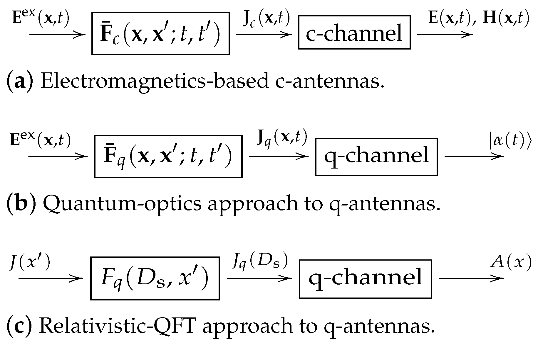
5.2. Comparative Analysis of the Three Fundamental Types of Antennas

At this point, it is instructive to give a bird’s eye view on the various genera of antenna theories available to us so far. Classical antennas (c-antennas) involve excitation with an external electric field E ex , which in turn induces a current on the antenna via the current Green’s function [28,46,47,48].22 This is illustrated in Figure 3a. Here, it is essential to note that the “system input” is a classical field, while the “system output” is also the classical radiated fields E and H . On the other hand, the quantum-optics approach to defining quantum antennas, which is the one currently most often mentioned in connection with applications to quantum communications [1,2,13], treats the input as a classical source while the output is a quantum state | α ( t ) [10,13,62,83]. This is illustrated in Figure 3b, where the q-antenna current Green’s function F ¯ q is still a classical function, just like the induced radiating current J q ( x ) .
Consider now the third type of antennas shown in Figure 3c. The input to the system J ( x ) (exactly like the previous two antenna types) is still a classical source, but now the radiating source J q ( D s ) is an operator that can describe quantum particles emission (quantum radiation) from within the q-antenna’s source spacetime region D s . In fact, we may rewrite (38) in the revealing integral form
J q ( D s ) : = x M 4 d 4 x F q ( D s , x ) J ( x ) ,
where the q-antenna current Green’s function in this case is simply given by
F q ( D s , x ) : = ϕ ( x ) , x D s , 0 , x D s .
Clearly, this is quite different from the two cases depicted in Figure 3a,b. In the case Figure 3c, captured by the expression (49), the current Green’s function itself is a quantum field, i.e., an operator-valued function on spacetime. The source J q reproduced by the Green’s function superposition integral is also an operator, and the ultimate “output” coming out from the relativistic QFT-based antenna system is the probability amplitude A ( q ) of annihilating a particle at some generic observation point x D r M 4 .

5.3. On the Causal Spacetime Structure of Radiation Emitted by Quantum Antenna Systems

In both special and general relativity, two events x and x with timelike distance, i.e., x x 2 > 0 , can be causally connected [51,53,84]. This has a direct and obvious implication for the general spacetime theory of q-antennas developed here.
  • Consider a point source case. Figure 4a indicates the future lightcone C x of the event located at x , i.e., the apex of the cone in the spacetime diagram given therein. Since we assume for simplicity that the operational principle behind our q-antenna-based communication link’s receiver is based on the process of annihilating the radiated particle at the observation point x, it follows that only receivers located inside the antenna causal lightcone C x can receive information from the point source.
  • For potential receivers located outside the antenna causal cone, it is not possible to transmit information at all, unless one admits some superluminal mechanism to be used for sending information, which is currently not accepted by majority of scientists.
These two observations above are enough to determine the causal structure of q-antennas for the case of point sources. However, since arbitrary sources can be constructed from assembling clusters of point sources, the argument can be expanded, as will be shown next.
For the case of continuous sources, the situation is qualitatively similar to the discrete scenario discussed above, but the detailed content of the antenna’s causal domain becomes somehow more complicated, since the situation strongly depends on the geometry of the source region in the former case. In Figure 4b, we schematically illustrate the problem when a generic continuous source J ( x ) is applied in the spacetime region D s M 4 . Since any current source function J ( x ) can be expanded into a continuous sum of point sources, as per the sifting property of delta functions
J ( x ) = x M 4 d 4 x   J ( x ) δ ( x x ) ,
one may then attempt to construct a causal lightcone for each point x D s , which is again denoted by C x . A continuum of causal cones is shown in Figure 4b where all cones appear to be aligned in parallel in spacetime because we ignore gravitational effects.
We now introduce the following construction of the antenna’s horizon causal structure, which is valid for both classical and quantum antennas:
Definition 5 (The antenna causal domain).
The antenna causal domain associated with a given source region D s , which we denote by C ( D s ) , is defined as simply the fusion (set-theoretic union) of all individual causal cones C x based on events located inside the source region x D s . That is, according to the recipe
C ( D s ) : = x D s C x .
The part of C ( D s ) that is solely due to future lightcones C x + is called the antenna future causal domain. Similarly, the components of C ( D s ) due to contributions emanating from past lightcones C x lead to the antenna past causal domain. Then, we have
C + ( D s ) : = x D s C x + ,   C ( D s ) : = x D s C x ,
and
C ( D s ) = C + ( D s ) C ( D s ) .
Note that the same constructions can be laid out for the receiving q-antenna case when the detector is in the receive domain D r .
Remark 14. 
Note that it is still possible to incorporate gravitation into our model, since the effect of gravitational fields is mainly to tilt the lightcones locally, where the tilting is directly determined by the gravitational potential/metric tensor g μ ν [41]. For applications of q-antennas in deep space communications, these gravitational effects may have to be taken into account. Consequently, the constructions provided by Definition 5 may become useful in astronomical and cosmological applications of either classical or quantum antennas. That is especially true when the large-scale structural impact of the gravitational field on a planned solar or even future interstellar communication links is important.
Remark 15. 
The causal domain C ( D s ) is a function of the source region D s . Moreover, it should be emphasized that in general, the antenna causal domain, as defined above, need not constitute a simple cone in itself. In addition, in principle, the receivers located inside C ( D s ) can receive information transmitted by radiation emitted from inside D s . On the other hand, noncausal receivers, e.g., see some cases schematically depicted in Figure 4b, can never receive information from an antenna system whose source is supported by the region D s .
Overall, the analysis above has highlighted an organic interlinking of spacetime with causality within the context of generic quantum communication systems utilizing quantum antennas. This suggests the need to pay closer attention to the global (i.e., topological) structure of spacetime domains when such future quantum technologies are incorporated in the analysis, design, and construction of long-distance space communication systems at the solar, extra-solar, astronomical, or even cosmological scales.

6. Quantum Antenna Radiation Patterns: Basic Constructions

6.1. Introduction

In contrast to classical antennas, q-antenna systems are intrinsically stochastic. The ultimate goal of a candidate q-antenna theory is to supply rules and guidelines for estimating probabilities of potential detection (reception) processes ideally enacted somewhere within the near or far spacetime zones of the quantum sources. In conventional antenna theory, certain quantities are fundamental for analyzing and designing functioning actual devices able to radiate power in real-life settings. These often include directivity, gain (preferably with a measure of radiation efficiency), and the array factor [27,33,35]. As will be illustrated in this section, it turns out that in q-antennas, there also exist close counterparts for many of the conventional characterization measures/concepts already in use in -c-antennas. However, there are also fundamental differences between c- and q-antennas in terms of the physical interpretation and meaning of the results thus obtained since, clearly, electromagnetic and quantum radiation are very distinct (though related) physical processes. For the purpose of constructing working definitions for directivity and gain functions suitable for q-antennas, we explore next some possible antenna radiation pattern constructions made available to us by the relativistic QFT approach proposed above.

6.2. The Probability Law of Producing Radiated Quantum States

From the general rules of QFT [54,56,57], the probability of measuring a particle with four-momentum q within the range Q M 4 is given by the integral of the square of the probability amplitude A ( q ) :
Pr { q Q } = 1 α q Q d 4 q   | A ( q ) | 2 = 1 α q Q d 3 q ( 2 π ) 3 | A ( q ) | 2 2 ω q ,
where Q R 3 is the projection of Q M 4 onto R 3 , and we made use of (A34) to derive the second equality in (54). The number α R + is a normalization constant defined by (57) inserted in order to ensure that the probability of any event is between 0 and 1.
Remark 16 (Relativistic normalization).
In writing the second equality in (54), a delta function
δ ( p 2 m 2 ) ,     p 0 > 0 ,
is included in the d 4 p -integral (54), i.e., the mass shell condition expressed by the dispersion relation (A27); see Appendix G for more details on this background.
Remark 17 (Probabilistic normalization).
The correct relativistic normalization of the four-momentum kets | p and | q , e.g., see relations such as (A38), which we have been already utilizing from the outset, does not automatically ensure the required probability normalization condition
Pr { q M 4 } = 1 α q M 4 d 4 q | A ( q ) | 2 = 1 .
The latter is in fact a consequence of the normalization in (54) by
α : = q M 4 d 4 q | A ( q ) | 2 ,
whenever the integral converges.
The normalization condition (56) is not a consequence of the completeness relation of the Lorentz momentum states (A38), but it should be enforced by hand in order to extract useful probability statements from the theory [85]. However, it should be stressed that the normalization integral (56) for the q-states is not convergent in the usual sense since exact continuous momentum states such as | q or | q are unormalizable [52,54,86]. For more detailed information about the proper rigorous mathematical theories that can deal with problems involving continuous states, see [37,55,67,79]. In practice, we seldom need to directly compute continuous state representation, since one always works with “discretized states”, where momentum or wavevectors are measured in a finite range [2,87]. The set of all such finite-range states is normalizable [54]. Therefore, whenever expressions such as (56) are encountered, they should be understood in the above of sense of being approximated by discrete sum after which the normalization to unity becomes correct. Nevertheless, for some choices of A ( q ) , for example the point source with A ( q ) = 1 , the integral (56) diverges regardless of whether one works with continuous or discretized state representations. This is an example of the persistent and well-known problem of ultraviolet (UV) divergences in QFT [38]. However, this problem is not a major issue in q-antenna theory, since in practical settings, one often requires a smoothly switchable source. In such types of source systems, the Fourier amplitudes of the spacetime source function decay fast enough in momentum space in order to secure the convergence of infinite spectral integrals such as (56). For in-depth discussion of this scenario backed by several examples taken from the area of high-energy physics, see Coleman’s lectures [38].
We next give a few examples to illustrate this formulation.
Example 2 (General quantum source’s radiation probability law at a particular momentum).
First, we construct a suitable probabilistic representation of a point source radiation function. Introduce the Euclidean ball
Q ( q 0 , ε ) : = { q R 3 , q q 0 < ε } ,
where q 0 R 3 , while ε R + is very small. (The norm |   ·   | is that inherited from the standard Euclidean metric on R 3 ). The probability of measuring a momentum q in the ball Q ( q 0 , ε ) is given by
Pr { q Q ( q 0 , ε ) } = 1 α p Q ( q 0 , ε ) d 3 q ( 2 π ) 3 | A ( q ) | 2 2 ω q ( 4 / 3 ) π ε 3 α ( 2 π ) 3 | A ( q 0 ) | 2 2 ω q 0 = ε 3 12 π 2 α | A ( q 0 ) | 2 2 ω q 0 ,
where ( 4 / 3 ) π ε 3 is the volume of the ball Q ( q 0 , ε ) centered at q 0 with radius ε . Therefore, the expression (59) gives the probability of measuring a momentum p = q 0 after exciting the ground state | 0 of the q-antenna to a higher-energy state | q 0 . It is completely general, regardless of how the vacuum state was excited.
Example 3 (Point source quantum radiation probability model).
Let us apply the rule (54) to the single quantum source probability amplitude (25). By treating (25) as a special case of (54), we find that for a point quantum source firing at the spacetime point x , the probability amplitude is A ( q ) = 1 ; hence, the total radiation probability is given by
Pr { q = q 0 } 1 α ε 3 12 π 2 ω q 0 = ε 3 12 π 2 α | q 0 | 2 + m 2 ,
after using the dispersion relation (A27). Since the expression (60) depends only on the amplitude of the momentum q 0 , not its direction, we conclude that the q-antenna with a single scalar quantum source is an isotropic radiator since it radiates its various four-momentum states | q in the same manner in all directions. This is not very surprising, since the quantum field of the q-antenna is scalar, and in classical antenna theory, a scalar point source is also isotropic [27].
Remark 18. 
From the antenna viewpoint, the examples above suggest that the quantum state of the q-antenna is inherently global and hence extendable everywhere. Therefore, we can not guarantee that the q-antenna has effectively radiated into every spacetime point until a concrete measurement process is performed at some position x, after which one may determine the probability of actual detection there using the receive antenna model with the help of the q-antenna Green’s function in Theorem 2. Such a process requires introducing a more sophisticated approach to measure probability amplitudes when the observation point is included as a parameter in the system. This subject will be taken up again in Section 6.4.

6.3. Constructing the Quantum Antenna Directivity Pattern

Our goal here is to estimate the directive properties of a continuous source J ( x ) located in the spacetime region D s . The probability amplitude of measuring the four-momentum q is denoted by A [ q ; J ( x ) , D s ] but will be abbreviated to A ( q ) whenever there is no confusion about the source. Our main tool here is the following theorem.
Theorem 5. 
Consider a q-antenna system J ( x ) , x D s M 4 . Let the corresponding probability amplitude be A ( q ) . Then, the following formula holds:
| A ( q ) | 2 = | J ( q , ω q ) | 2 ,
where J ( q ) is the spacetime Fourier transform of the radiating current source (A45).
Proof. 
See Appendix I.  □
Remark 19. 
Since there is a one-to-one (injective) mapping between the Lorentz four-momentum states q M 4 and the conventional three-momentum vectors q R 3 via the dispersion relation (A27), we may just write A ( q ) instead of A ( q , ω q ) .
Theorem 6. 
For the situation described in Theorem 5, the quantum radiation probability amplitude can be expressed as:
Pr k Q = 1 α k Q d 3 k ( 2 π ) 3 | J ( k ) | 2 2 ω k ,
for a generic three-dimensional region Q R 3 . Here, J ( k ) : = J ( k , ω ) is the momentum space Fourier transform of the source defined by (A45); see also Remark 19 on the reduced notation in momentum space used here.
Proof. 
Use the probability law (54) in (61) and make the replacement q k .  □
An immediate application of Theorem 6 is in expressing the total energy radiated by a quantum source directly in terms of the classical source function J ( x ) , as will be illustrated through the next example.
Example 4 (Total radiated energy and momentum of a q-antenna in momentum space).
The total energy radiated by the antenna in a momentum space region Q R 3 can be obtained by multiplying the probability of particle production in the infinitesimal momentum space volume d 3 k by the particle’s energy, which is ω k (or just ω k in natural units), and then integrating. With the help of (62), this procedure yields:
E Q = 1 2 k Q d 3 k ( 2 π ) 3 | J ( k ) | 2 ,
where E is the total energy. Similarly, the expected value of the total radiated momentum can be estimated via the formula
P [ Q ] = 1 2 k Q d 3 k ( 2 π ) 3 | J ( k ) | 2 k k 2 + m 2 ,
where use was made of the fact that the momentum of the particle excitation associated with the k th state is k (or k in natural units).
Remark 20. 
It is interesting to note that the momentum space energy pattern of the q-antenna (63) is similar to the energy directivity of a classical source in generic medium. For example, see how general formulas of directivity for classical radiators were constructed recently in momentum space for generic homogeneous nonlocal domains [71,72,73].
In order to put relation (62) into further practical use, we transform momentum representations into spherical coordinates so we may obtain some information about the directive properties of quantum radiating sources as illustrated by the following example.
Example 5 (Radiation angular directivity pattern of q-antennas in momentum space).
Let us express the wavevector k in terms of the spherical angular coordinates θ and φ by using the standard transformation
k ^ = k ^ ( Ω ) = x ^ 1 cos φ sin θ + x ^ 2 cos φ sin θ + x ^ 3 cos θ ,
where
Ω : = ( θ , φ ) , k ^ ( Ω ) : = k | k | .
Here, x ^ i , i = 1 , 2 , 3 , constitute a set of three mutually orthogonal Cartesian unit vectors. The angles 0 < φ < 2 π , 0 < θ < π determine the direction of the unit vector k ^ , or where the emitted quantum particle’s momentum p = k is pointing in three-dimensional space. Since physically and intuitively, one would expect that the directions in three-dimensional position space along which momenta tend to maximally flow also correspond to the directions toward which most of the particle ensemble’s energy and momentum are directed, we may use Theorem 6 in conjunction with (66) to estimate the quantum source’s directive properties in generic three-dimensional scenarios. A simple way to achieve this is by re-expressing (62) using (65) and (66), resulting in
Pr k [ k min , k max ] ,   Ω Ω 0 = 1 α k [ k min , k max ] Ω Ω 0 d k   d Ω   k 2 sin θ ( 2 π ) 3 J k , k ^ ( Ω ) 2 2 k 2 + m 2 ,
where
k : = | k | , d Ω : = d θ d φ .
The angular set Ω 0 in (67) is the three-dimensional (solid) angular sector inside where one is interested in characterizing the radiating quantum antenna system.
Remark 21. 
It is important not to confuse k R + , defined by (68), with the four-vector k = k μ M 4 (Appendix B). In this section, we use the shorthand notation (68) in order to simplify the presentation.
Inspired by the expression (67), we may then introduce the following definition of momentum space directivity for quantum antennas:
Definition 6 (Quantum antenna directivity in momentum space).
The momentum space directivity of a q-antenna with source function J ( x ) , x D s is defined as the following angular function
D ( φ , θ ; k ) : = 1 α k k 2 sin θ ( 2 π ) 3 J k , k ^ ( φ , θ ) 2 2 k 2 + m 2 ,
where
α k : = 1 4 π 4 π d Ω k 2 sin θ ( 2 π ) 3 J k , k ^ ( φ , θ ) 2 2 k 2 + m 2
is a positive momentum-dependent probability noramalization constant.
Expressed in terms of the momentum-space-type directivity (69), the total probability in (62) may be be put into the more compact form
Pr k [ k min , k max ] ,   Ω Ω 0 = k [ k min , k max ] d k α k α Ω Ω 0 d Ω   D ( φ , θ ; k ) .
The last expression explains the physical motivation behind Definition 6. Moreover, the following two remarks explain more about the engineering background to directivity concepts in antenna theory motivating the above definition itself.
Remark 22. 
It is evident then from (71) that for a given k ^ , the function D ( k , k ^ ) is the angular probability density in the momentum space variable k. On the other hand, the mathematical dependence of D ( k , k ^ ) on the angles φ and θ provides information on how the emitted quantum particles tend to flow along different directions in space. This is why D does indeed behave as a momentum-space radiation pattern (probability per unit momentum per solid angle).
Remark 23. 
The positive number α k is inserted into (69) in order to ensure that the total probability of radiation at all angles, evaluated at a single radial momentum value k, is equal to that of an isotropic source.23 Intuitively, α k represents the total radiation angular density emitted by the q-antenna, so the ratio D given by (69) is the relative radiation intensity along one direction with respect to a standard isotropic source
D 0 : = P 0 4 π ,
where P 0 is the constant radiation angular probability of such an isotropic reference antenna whose radiation angualr density is D 0 . That is, we have
Ω 4 π d Ω   D ( φ , θ ; k ) = 4 π D 0 ,
as expected from a typical directivity expression [35]. Physically, the ratio 4 π α k / α in (71) represents the fraction of the total quantum radiation contained in a sphere with radius k in momentum space relative to the total radiation obtained by including contributions coming from all values of the momentum magnitude k : = | k | . The ability of a source to direct power along certain directions is measured by angle-dependent generalizations of such total ratios. Then, Definition 6 of the q-antenna directivity is a natural generalization of the corresponding definition in classical antenna theory as traditionally presented in texts such as [27,35].

6.4. The Probability Law of Receiving Radiated Quantum States: Source-Receiver Coupling Gain Estimation

Consider the configuration shown in Figure 5. The quantum antenna communication system is characterized by the gain functional
G : X × X C , G = G [ J s , J r ] ,
which is a bilinear functional in the source and receiver currents J s ( x ) X , x D s , and J r ( x ) X , x D r , respectively. Here, X is the space of real-valued functions on the four-dimensional domains D s , r M 4 . The complex number G gives the probability amplitude of information transmission (coupling amplitude) between source and receiver. This gain plays the role of “transmission coefficient” or the “coupling coefficient” often used in conventional electromagnetic communication systems, e.g., see [33,88]. From the fundamental theory of quantum antennas developed above, we may easily deduce the general expression of this functional by simply treating the receiver as a source with the “quantum reverse” process of that of the transmitter, i.e., the dual of the transmitter problem, e.g., by converting kets to bras, taking adjoints, complex conjugates, etc. Since for real sources and receiver currents J r , s ( x ) , the problem is fully reciprocal,24 we can immediately write down the q-antenna system gain expression as follows:
G = 0 | x D r d 4 x x D s d 4 x   J r ( x ) T ϕ ( x ) ϕ ( x ) J s ( x ) | 0 ,
where (43) was used to realize the transmitter, and a similar form was adapted for the receiver.
Example 6 (Construction of practical angular gain pattern in q-antenna systems).
We will use the general relativistic expression (75) in order to construct an angular expression characterizing quantum radiation for possible use in practical settings. To do that, we first need to break relativistic covariance in order to simplify the problem and facilitate calculations. The most natural choice for a preferred frame is to use a coordinate system at rest with either the lab frame of the transmitter or the receiver. We choose the source frame below. Consider a standard test receiver to be used for performing quantum measurement on the radiation emitted by the source J s ( x , t ) , where x S s , and S s is the spatial support of the source region. The receiver spatial region is S r , and its strength is given by J r ( x , t ) . Both t and t will be measured with a single clock at rest in the source lab frame. Let the test (receiver) current be reduced to a concentrated delta source
J r ( x ) = J r ( x , t ) = δ ( x x r ) J r ( t ) ,     t T r .
That is, we measure the response at a sharp spatial location x r , while we impose the receiver function restriction J r ( t ) on the time measurement interval T r . We can use (66) to express the position vectors as
x r = | x r | x ^ r ( Ω ) ,
where the unit angle-only dependent unit vector x ^ r is defined by
x ^ r ( Ω ) : = x r | x r | .
By substituting the relations (76), (77), and (78) into the gain Formula (75), the following angular expression is obtained:
G ( Ω ; | x r | ) = x S s ,   t T s d 3 x d t   G q a ( Ω ; | x r | , x ) J s ( x ) ,
where
G q a ( Ω ; | x r | , x ) : = t T r d t   G q ( | x r | x ^ r ( Ω ) x ; t t ) J r ( t ) ,
and the notation of (27) was used. The integral (80) can be computed numerically for known current source distributions J s ( x ) by using the special functions representation of the Feynman propagator G q ( x x ) given in Appendix H.
Remark 24. 
We note that the q-antenna system gain Function (79) depends on the distance between the source and the receiver in addition to the angles. In general, one studies the asymptotic behavior of G q a ( Ω ; | x r | , x ) in the long distance limit | x r | , with the hope that this behaves as | x r | n , with n often a small integer (usually 1 or 2). From the asymptotic limits of the special functions used in Appendix H, some possible relations could be derived using the bessel function large argument approximation, which in turn then might be further utilized in order to eliminate the dependence on the radial distance in the gain pattern (79). However, such detailed computational considerations are outside the scope of this paper, which is mainly focused on the general fundamental theory.

7. Conclusions

We developed foundations for quantum antenna theory using the relativistic framework of quantum field theory (QFT) with emphasis on the source–sink (transmitter–receiver) model for potential applications to quantum communication systems. The QFT-based q-antenna is the most general type of antenna systems because it includes both the classical and quantum-optics-based q-antennas as special cases. In addition, relativistic q-antennas can accommodate a wider range of physical processes, since the same theory may deal with massive or massless particles and for different spins. These types of q-antennas, the most general to date, appear to enjoy the distinction of exhibiting a current Green’s function that is itself a quantum field, which we dubbed before the quantum source of the antenna system, i.e., the field ϕ ( x ) as per (49). We have illustrated the theory mostly with the specific example of the neutral Klein–Gordon field because of its simplicity and importance for building the general solution to other, more complex problems. In particular, we have shown how in the linear quantum antenna model, one may directly construct quantum radiation directivity and gain measures that somehow resemble their counterparts in classical antenna theory. A future research based on the present theory would proceed to construct more concrete radiation models for quantum fields such as the Proca field (massive electromagnetism), the Maxwell–Dirac field (quantum electrodynamics), the graviton field (gravitational antennas), and possibly other types. Then, the present paper attempted to provide a first sketch of a possible general theory that may blend all these distinct phenomena, where our key idea was that relativistic QFT supplies precisely a promising such unifying theoretical framework.

Funding

This research received no external funding.

Institutional Review Board Statement

Not applicable.

Informed Consent Statement

Not applicable.

Data Availability Statement

Not applicable.

Conflicts of Interest

The author declares no conflict of interest.

Abbreviations

The following abbreviations are used in this manuscript:
QFTQuantum field theory
QMQuantum mechanics
SRSpecial relativity
c-antennaClassical antenna
q-antennaQuantum antenna
q-radiationQuantum radiation
q-stateQuantum state
q-sourceQuantum source
c-sourceClassical source
EMElectromagnetic/Electromagnetics
ACGFAntenna current Green’s function

Appendix A. Classical Antenna Theory

Let the source or current Green’s function be the dyadic tensor F ¯ ( x , x , t t ) [28,46,47,48,89]. The forward Green’s function is the standard retarded radiation Green’s function G ¯ ( x x , t t ) [49]. Then, we have the following two fundamental relations [28,90]:
J ( x , t ) = S d 2 x   d t   F ¯ ( x , x , t t ) · E ex ( x , t ) ,
E ( x , t ) = S d 3 x   d t   G ¯ ( x , x , t t ) · J ( x , t ) ,
where E ex ( x , t ) is the excitation electric field, J ( x , t ) is the radiating antenna current on its compact surface S supporting the electromagnetic boundary conditions, and E ( x , t ) is the radiated field. For simplicity, we assume perfect-electric conducting (PEC) antennas where the magnetic field does not contribute to the current Green’s function. Another radiating Green’s functions similar to G ¯ ( x , x , t t ) is needed in expressions such as (A2) in order to obtain the magnetic field B ( x , t ) , which is always present in any radiation problem beside the electric field; see [89,90,91] for more details and applications.
The relation (A1) captures the antenna’s fundamental Mode A, where a source field E ex ( x , t ) produces a radiating current via the current Green’s function F ¯ ( x , x , t t ) , which in turn generates the radiated fields E ( x , t ) and B ( x , t ) throughout the region exterior to the surface S. To complete the antenna-based wireless communication system, a third Mode C, where a receiving (Rx) antenna, placed at some distance from S, interacts with the radiated field in order to produce an observable receive port current J rx ( x ) by means of the formula
J rx ( x , t ) = S rx d 2 x d t   F ¯ rx ( x , x , t t ) · E ( x , t ) ,
where F ¯ rx ( x , x , t t ) is the receive current Green’s function, which is generally different from the transmit (Tx) current Green’s function F ¯ ( x , x , t t ) . The three relations and Green’s functions in (A1)–(A3) fully describe the antenna system in classical electromagnetic theory [92], with obvious generalization to magnetic field interactions included in essentially the same logic [90].

Appendix B. The Relativistic Four-Vector Formalism

In special relativity, everything takes place in the four-dimensional Minkowski spacetime, denoted by M 4 , a linear vector space with a special metric, the Lorentz metric, given by
g μ ν = 1 0 0 0 0 1 0 0 0 0 1 0 0 0 0 1 .
We follow the standard convention of denoting spacetime indices using Greek letters μ = 0 , 1 , 2 , 3 , with the time-like component always given the 0th index and the space-like part denoted by Roman letter. Four vectors with upper and lower indices are dual vectors. The converse of the metric tensor g μ ν is g μ ν , i.e., g μ ν g μ ν = δ μ ν , where δ μ ν is the Kronecker delta function. Note that summation over repeated indices is implied (the Einstein repeated index convention). In general, we raise or lower indices by contracting with the fundamental tensor in relations such as a μ = g μ ν a ν or a μ = g μ ν a ν . From this we can see, for example, that a 0 = a 0 , and a i = a i . The dot product between two four vectors a μ and b μ is defined as a μ b μ : = a μ g μ ν b ν = g μ ν a μ b ν . We also write this as a · b : = a μ b μ where a and b stands for the four-vectors a μ and b μ . In particular, the all-important inner product p · x between four-momentum p μ and spacetime position x μ , given by
p · x = p μ x μ = ω t k · x ,
will be used frequently. Note that in M 4 , the proper “differential operators four-vectors” are given by μ = ( / t , ) and μ = ( / t , ) . Table A1 provides a compact summary of the main relativistic formulas.
Table A1. List of main basic relativistic relations in the Natural Units.
QuantityExpression
p (particle momentum) p = k
E p (particle energy) E p = ω p = ω k
Relativistic dispersion relation E p 2 = p 2 + m 2
μ (four-vector differential operator) μ = ( / t , )
x μ (position four-vector) x μ = ( t , x )
k μ (relativistic wavevector) k μ = ( ω , k )
p μ (photon four-momentum vector) p μ = ( E p , p ) = k μ
g μ ν (Lorentz metric tensor) g μ ν = diag ( 1 , 1 , 1 , 1 )
p μ x μ (four-vector inner product) p μ x μ = g μ ν p μ x ν = ω t k   ·   x

Appendix C. Natural Units

In relativistic quantum field theory, it is customary to use a system of units in which = 1 , c = 1 . Here, the action S is dimensionless. Mass, energy, wavevector, and momentum have the same dimension, which is the inverse of the dimension of length and time:
[ mass ] = [ energy ] = [ momentum ] = [ length ] 1 = [ time ] 1 .
Therefore, the physics of the world is reduced to measurements in two units, length and time. Moreover, in four dimensions, the creation and annihilation operators have the dimension of an inverse energy, i.e., [ a p ] = [ a p ] = [ energy ] 1 .

Appendix D. Dirac Interaction Picture

Consider a Hamiltonian H that can be written as
H = H 0 + H ( t ) ,
where H 0 is the free Hamiltonian of the system (time-independent function), while H ( t ) is the interaction (time-dependent) Hamiltonian, which is usually assumed to be turned on at a specific time point. In the Dirac picture, our goal is to decouple the free dynamics of the system, i.e., that governed by a Hamiltonian of the form H = H 0 (no interaction or H = 0 ), from the pure interaction component, i.e., that which is solely due to the term H in the actual full Hamiltonian (A7). Now, let us define the following time-dependent operator
O I ( t ) : = e i H 0 t O S e i H 0 t ,
where O S is the Schrodinger picture (time-independent) operator. Differentiating (A8) with respect to time, we obtain the Heisenberg equation of motion
i d d t O I ( t ) = [ O , H 0 ] .
Therefore, the interaction picture operator O I ( t ) evolves in time according to the exact same law corresponding to the case when the full Hamiltonian is just the free part, i.e., H = H 0 .
What about the evolution of the interaction picture state, which will be denoted by ψ I ( t ) ? To find out, note that all different pictures, the Schrodinger, Heisenberg, and Dirac, must agree on probability amplitudes. Therefore, for any two pairs of Schrodinger and Dirac states ψ S ( t ) , φ S ( t ) , and ψ I ( t ) , φ I ( t ) , respectively, the matrix elements in both pictures must be identical. Formally, we express this by the condition
ψ S ( t ) | O S φ S ( t ) = ψ I ( t ) | O I ( t ) φ I ( t ) = ψ I ( t ) e i H 0 t | O S e i H 0 t φ I ( t ) .
Clearly, this implies that we should define the Dirac (interaction) state by
| ψ I ( t ) : = e i H 0 t | ψ S ( t ) .
To find out how this state evolves, we differentiate with respect to time, obtaining
i d d t | ψ I ( t ) = H 0 + i d d t | ψ S ( t ) = H | ψ S ( t )
where we have made use of the Schrodinger equation
i d d t | ψ S ( t ) = H | ψ S ( t )
and the form (A7). Finally, using the definition (A11) of the interacting picture state, the relation (A12) becomes
i d d t | ψ I ( t ) = H I ( t ) | ψ I ( t ) ,
where the Dirac picture interacting Hamiltonian H I is given by
H I ( t ) : = e i H 0 t H ( t ) e i H 0 t .
Let us summarize the main features of this Dirac picture:
  • In the Schrodinger picture, the state evolves in time according to the full Hamiltonian while the operators are constant.
  • In the Heisenberg picture, the state is constant (time-independent), but the operator evolves according to the full Hamiltonian.
  • In the Dirac picture, both state and operators evolve with time. However, the time evolution is decoupled into two distinct and independent components. First, all interaction (Dirac) picture operators evolve according to the free Hamiltonian as per the corresponding Heisenberg Equation (A9). Second, the Dirac state | ψ I ( t ) evolves independently according to the dynamic Equation (A14).
Therefore, the main advantage of the Dirac picture is that we can concentrate on the essential aspects of interaction as encoded in the Schrodinger-like dynamic Equation (A14). In this equation, Schrodinger or Heisenberg states and operators can be obtained using the usual transformation formula. On the other hand, note that operators in the Dirac picture, including in particular the interaction Hamiltonian (A15), all evolve according to the free evolution law (A9). In this case, this becomes
i d d t H I ( t ) = [ H I ( t ) , H 0 ] ,
which says that all quantum fields inside H are to be evolved under the free Hamiltonian H 0 in order to obtain the dynamics of H I ( t ) .
Let us finally solve the dynamical evolution Equation (A14). To do so, introduce the time-ordering symbol  T defined by
T [ A ( t 1 ) B ( t 2 ) ] : = A ( t 1 ) B ( t 2 ) , t 1 > t 2 , B ( t 2 ) A ( t 1 ) , t 2 > t 1 .
Then, the general solution of (A14) can be expressed in terms of the evolution operator  P ( t 2 , t 1 ) , which evolves that initial state | ψ ( t 1 ) to the final state | ψ ( t 2 ) via the operator relation
| ψ I ( t 2 ) = P ( t 2 , t 1 ) | ψ I ( t 1 ) ,
where
P ( t 2 , t 1 ) : = T e i t 1 t 2 d t H I ( t ) .
The reader may verify that (A18) and (A19) indeed solves (A14) by direct substitution. Note that all operators inside the ordered exponential symbol T commute with each other.

Appendix E. On the Background to Theorem

The complete and most general proof of Theorem 1 can be obtained by utilizing a generalized framework, that of algebraic quantum field theory [37,78]. The expansion (15) can be shown to be derivable from a suitable perturbative algebraic quantum field theory, e.g., the recent approach [93]. The advantage of choosing such a method is that one does not need to assume a concrete Lagrangian from the beginning but rather proceed to work directly with algebras of quantum fields and then use the structure of these algebras in order to construct the entire theory, including the quantum states themselves, which are generated internally. However, since the mathematical details are extensive, the full treatment will be presented in a separate paper. Nevertheless, note that special cases of Theorem 1 have already appeared repeatedly in the literature, though in quite different applications and within distinct contexts. For example, a special case of (15) seems to have been discussed by Coleman in his analysis of perturbation calculations in scattering theory [38]. Moreover, a less general form of the expansion (15), known as the Volterra series, is often presented in several textbooks on QFT when discussing the evaluation of the vacuum expectation persistence function in terms of the higher-point Green’s (correlation) functions of the quantum field, e.g., see [38,54,55,56,57,58,67].

Appendix F. The Neutral Klein–Gordon Field Theory

A massive neutral Klein–Gordon field with mass m can be fully captured by a real scalar field ϕ ( x ) whose Lagrangian density is given by [38,54,56,75]
L ( x ) = 1 2 μ μ ϕ ( x ) + 1 2 m 2 ϕ ( x ) 2 ,
with the corresponding action integral being
S = d 4 x   L ( x ) .
The Euler–Lagrange equation of motion
δ S δ ϕ ( x ) = 0
yields the field equation
μ μ ϕ ( x ) + m 2 = 0 ,
which is the relativistic wave equation of a particle the Klein–Gordon equation [38,75].
Note that within the framework of standard quantum field theory (QFT), fields are promoted to operators expanded in terms of plane-wave modes of the form
operator × exp ( i p μ x μ ) ,
where the “operator” is either creation a p or annihilation a p operator (for particles or antiparticles). Note further that by convention, the plane wave
exp ( i p μ x μ ) = exp i ( E p t p   ·   x )
is taken to encode an incoming wave/particle with momentum p/wavevector k and energy E p /frequency ω [38]. In the unified language of QFT, we say that the plane wave encodes a particle/antiparticle in a pure momentum state p. Within this convention, the energy/frequency of a particle/wave is always positive.25
By applying the canonical quantization algorithm [38] (see review in Appendix G), the quantum field ϕ ( x ) may be expanded into a continuous sum of spacetime modes (plane waves) as follows
ϕ ( x ) = p R 3 d 3 p ( 2 π ) 3 / 2 1 ( 2 ω p ) 1 / 2 a p e i p μ x μ + a p e i p μ x μ ,
with the dispersion relation (in natural units)
E p = ω p = ω k = + | p | 2 + m 2 = + | k | 2 + m 2 .
The creation and annihilation operators a p and a p , respectively, obey the standard canonical commutation relations
[ a p , a p ] = 0 ,   [ a p , a p ] = 0 ,   [ a p , a p ] = δ ( p p ) ,
where δ is the Dirac delta function.

Appendix G. The Relativistic Field-Theoretic Canonical Quantization Algorithm

The general canonical quantization algorithm is shown in Algorithm A1, where we leave the nature of the field (scalar, vector, spin type, tensor, etc.) unspecified. In what follows, the detailed quantization algorithm applies to our main type of fields in this paper, i.e., the massive spin-0 scalar field ϕ ( x ) . Recall that in nonrelativistic quantum theory, a generic operator can be Fourier expanded in terms of creation and annihilation operators a p and a p , respectively. For instance, a generic scalar quantum field ϕ ( x ) is expected to be written as
ϕ ( x ) = p R 3 d 3 p ( 2 π ) 3 a p e i p μ x μ + a p e i p μ x μ .
Unfortunately, clearly, this expression is not Lorentz invariant because of the use of the non-Lorentz invariant integration measure d 3 p . We review below how Lorentz-invariant quantum states | p may be redefined so that Fourier expansions like (A29) can be made manifestly covariant.
In order to expand the quantum field into a proper continuum of plane-wave modes of the form exp ( ± i p μ x μ ) , we will need to integrate over all four-vector momenta p μ , i.e., perform four-dimensional integrals over p and E p (or equivalently k and ω ). However, for massive particles in general, and Proca waves in particular [94], there is a definite relation between momentum/wavevector and energy/frequency, so the integral over d 3 p might appear at first sight to be essentially reducible to d 3 p , while E p is computed from E p 2 = p 2 + m 2 . However, the problem is that the differential element d 3 p is not Lorentz invariant, so there is a need to automatically enforce Lorentz invariance in our quantization rules. In this paper, we adopt the computationally efficient method of applying normalizing factors to quantum states right from the beginning. The main idea is to produce Lorentz-invariant momentum quantum states and use them to expand the quantum fields.
The essence of the method of normalizing factors is to perform a transformation of the form
p R 3 d 3 p   p M 4 d 4 p
taking us from the non-Lorentz invariant space R 3 to Minkowski space M 4 , where d 4 p is clearly invariant since p : = p μ = ( p 0 , p ) . However, note that the mass shell condition
p 2 : = p μ p μ = m 2
forces this integration to remain on the cone defined by equations of this type, i.e., a four-submanifold embedded into M 4 whose equation is (A31). Then, we may write
d 4 p = d 3 p δ p 2 m 2 Θ p 0 ,
where Θ ( · ) is the Heaviside unit step function, which is inserted by hand in order to prevent the appearance of negative energies. It can be shown that [38,76]
δ p 2 m 2 Θ p 0 = ( 1 / 2 E p ) δ ( E E p ) Θ ( E p ) ,
and hence, we conclude
p M 4 d 4 p ( 2 π ) 3 = p R 3 d 3 p ( 2 π ) 3 1 2 E p ,
where the factor 1 / ( 2 π ) 3 was intentionally inserted in order to make the final integral looks like an inverse Fourier transform (this inserted factor will be compensated for shortly when we define the normalizing factors of the Lorentz-invariant state | p ). Therefore, we have managed then to reduce a four-dimensional integration in M 4 into a regular volume integral in R 3 . Note that by writing the RHS of in (A34) without δ ( E E p ) Θ p 0 , it is to be implicitly understood that – algorithmically speaking – every appearance of E or ω in the various possible expressions placed to the right of the integral operator sign d 3 p should be automatically replaced by + E p or + ω k .
A Lorentz-invariant momentum state | p should be constructed from the standard three-vector momentum states | p , which obey the normalization rule
p | p = δ ( p p ) .
The most obvious construction of the Lorentz-invariant momentum state then is
| p : = ( 2 π ) 3 / 2 ( 2 E p ) 1 / 2 | p .
For example, the inner product of such states is
p | p = ( 2 π ) 3 ( 2 E p ) δ ( p p ) .
The definition (A36) can be readily used to yield the desired Lorentz-invariant completeness relation
𝟙 = p R 3 d 3 p ( 2 π ) 3 1 2 E p Lorentz   measure | p p | ,
where 𝟙 is the unity operator. The computational utility of the method of normalizing factors stems from the fact that a completeness relation originally holding for all states { | p , p M 4 } in the full four-dimensional Minkowski space is now reduced to carrying out integration in the regular Euclidean space R 3 . However, the price to be paid for such simplification is that a momentum-dependent factor 1 / 2 E p must be inserted into the integrand of the reduced integral, which slightly complicates the evaluation of various related expressions such as probability amplitudes.
Finally, we can create the Lorentz state by applying a new normalized creation operator b p to the ground or vacuum state | 0 , i.e., | p = b p | 0 and b p | 0 = 0 . Based on (A36), we expect
b p = ( 2 π ) 3 / 2 ( 2 E p ) 1 / 2 a p ,     b p = ( 2 π ) 3 / 2 ( 2 E p ) 1 / 2 a p .
The field expansion now, based on (A38), becomes
ϕ ( x ) = p R 3 d 3 p ( 2 π ) 3 1 2 E p b p e i p μ x μ + b p e i p μ x μ ,
which after using (A39) leads to
ϕ ( x ) = p R 3 d 3 p ( 2 π ) 3 / 2 1 ( 2 E p ) 1 / 2 a p e i p μ x μ + a p e i p μ x μ .
Algorithm A1 The Canonical Quantization Algorithm (General Formulation).
1:
Start with a Lagrangian density L .
2:
Find the momentum density. From this knowledge, construct the Hamiltonian.
3:
Promote the field and the corresponding momentum variables to operator-valued fields. Apply the standard commutation relations.
4:
Expand the quantum fields into sums of plane waves with creation and annihilation operator amplitudes.
5:
Evaluate the Hamiltonian operator in terms of the creation and annihilation operators and put in in the normal ordering form.

Appendix H. On the Numerical Evaluation of the Propagator

For the scalar massive or massless field theory considered above, the Green’s Function (29) can be evaluated in closed analytical forms after regulating the integral by inserting small imaginary number i ϵ at proper locations in the integrand in order to ensure convergence (causality consideration, e.g., see [54,55]). The final expressions are given by [56]
G q ( x , x ) = i m 8 π H 1 ( 2 ) ( m | x x | ) m | x x | , m 0 , 1 4 π 2 1 x x 2 i ϵ , m = 0 .
Here, the distance x x is computed in Minkowski spacetime M 4 with the metric tensor g μ ν , i.e, the relation
| x x | 2 = ( t t ) 2 | r r | 2 .
The Hankel function of the second kind H ν ( 2 ) is defined as
H ν ( 2 ) ( x ) : = J ν ( x ) ± i N ν ( x ) ,
where J ν and N ν are the Bessel and Neumann functions, respectively [95,96].

Appendix I. Proof of Relation

Proof of Relation (61), when there is a source J ( x ) , x D s , then the actual radiated (quantum) state of the q-antenna system is obtained by applying the operator
x D s d 4 x J ( x ) ϕ ( x )
on the ground state | 0 in order to create the following one-particle excited state
x D s d 4 x J ( x ) ϕ ( x ) | 0 .
To measure the probability of having a four-momentum state | q in the previous excited q-antenna state, we compute the source probability amplitude A [ q ; J ( x ) , D s ] as follows:
A [ q ; J ( x ) , D s ] : = q | x D s d 4 x J ( x ) ϕ ( x ) | 0 = p R 3 d 3 p ( 2 π ) 3 / 2 ( 2 ω p ) 1 / 2 x D s d 4 x J ( x ) e i p μ x μ q | p = p R 3 d 3 p ( 2 π ) 3 / 2 ( 2 ω p ) 1 / 2 J ( p ) δ ( q p ) ( 2 π ) 3 / 2 ( 2 ω p ) 1 / 2 = J ( q ) | q 0 = ω q = J ( q , ω q ) ,
where
J ( k ) : = x D s d 4 x   J ( x ) e i k μ x μ = x R 3 d 3 x t R d t   J ( x , t ) e i ( ω t k   ·   x )
is the four-dimensional (Minkowski) Fourier transform in spacetime. The second line in (A45) follows from using the momentum-space expansion of the source field ϕ ( x ) given by (A26), while in the third line, we used the normalized four-momentum state inner product formula
q | p = ( 2 π ) 3 / 2 ( 2 ω p ) 1 / 2 δ ( q p ) ,
then proceeded to evaluate the trivial resulting integral over a delta function.

Notes

1
Other possible long-term aims behind the spacetime theory of q-antennas proposed below include the stimulation of fruitful collaboration between theoreticians, especially those working on problems related to foundations, and applied quantum physicists and engineers, whose attention is often more focused on algorithmic and physical-layer applications, e.g., quantum communications, cryptography, computing, and so on.
2
Maxwell’s equations in vacuo are exactly linear [49,51]; a photon does not self-interact with itself [52]. As in classical antenna theory, in the proposed quantum antenna theory given here, all nonlinearities are relegated to production of the source J ( x ) itself. Well-known examples include gun diodes (microwaves) and laser devices (optics), where the diode itself is nonlinear but the relation between the current or field as external source and the fields radiated into vacuum is linear. The physical nonlinear processes behind the source function J ( x ) itself are outside the scope of the proposed theory.
3
Otherwise, relativistic causality would preclude information transfer [51]. In general, there is an agreement in the literature that entanglement-based quantum communication links cannot transmit information at superluminal speeds even though the quantum correlations between entangled states persists at spacelike separated terminals [2,4].
4
This is a realistic assumption in our model, in conformity with the common practical situation where typical classical or quantum sources are supported by bounded spatial domains and radiate within a finite time interval while practical measurement times are also bounded.
5
The propagators coincide with well-known Green’s functions in the case of free fields. For interacting field theories, the propagators are not in general known, but viable approximations can be estimated using perturbation theory, in which the free-field Green’s function is used as a fundamental building block in order to compute more complex higher-order interaction processes [54,55,56,57,58,59,60].
6
By effective path, we just mean the spacetime trajectory in the Feynman’s path integral expansion of the propagator that contributes most to the total probability amplitude, e.g., see [57].
7
8
Interaction is a more general concept than quantum correlation, since two uncorrelated objects could interact, where in this case, the interaction terms are just the multiplication of the strengths of each process while the two remain, at least stochastically speaking, independent. An example illustrating this will be given shortly.
9
Nowadays, such many-body effects are approached in the modern literature on condensed-matter physics, e.g., through the elaborate and elegant language of many-point correlation or Green’s functions in QFT [59,60,61].
10
In QFT, integrals such as (20) are handled using four-point Green’s functions of the form G ( 4 ) ( x 3 , x 4 , x 1 , x 2 ), where the latter is called the four-point correlation (Green’s) function [54,55,57]. In our case, we just choose x 3 = x 4 = x , since x is the common observation point of the receiving q-antenna system.
11
The realization of the need to eventually differentiate a purely classical source function from within any stochastic system (including quantum systems) was originally proposed within the context of quantum optics in the 1960s [62].
12
For the purposes of illustrating the main ideas of q-antenna systems, this assumption simplifies considerably the presentation, but the main ideas related to q-antennas are unchanged when more complicated field theories are considered such as spin-1 and spin- 1 / 2 theories.
13
For additional information on the physical processes modeled by a Klein–Gordon quantum field, see [74,75].
14
For a more detailed discussion of relativistic QFT, see [38,76].
15
The generation of ϕ ( x ) itself is not treated here for simplicity. However, note that computing the quantized fields of coupled matter–field systems is a fairly well-developed area in the physics and engineering literature, mostly using the methods of perturbation theory [38,54,55,67,77]. On the other hand, in this paper, our main focus is on how to deploy an already given or generated quantum field ϕ ( x ) in order to construct the radiation pattern and the Green’s function of a q-antenna system for use in applications in controlled radiation of quantum states.
16
When reworked in the full momentum space p M 4 , the integral (21) becomes even more interesting, both computationally and conceptually, since one can show then that point source excitations lead to the production of virtual (off-mass-shell) particles [38,57]. However, we will not make use of these expansions in the present paper though they are expected to play an important role in developing the near-field theory of radiating quantum source systems.
17
The concept of particle localization in QFT is difficult both philosophically and mathematically, and several approaches have been proposed in the literature so far, apparently with no universal agreement on the ontological status of particles in field quantization. Such more advanced issues do not affect the practically oriented theory of quantum antennas developed in this paper. For some in-depth discussion of localization in field theory, see [37,78].
18
Recall that in QFT, antiparticles are interpreted as particles moving backward in time [57,58].
19
Momentum space means either p R 3 or p M 4 . In this paper, whenever the term momentum space is invoked, it is to be understood that we will mostly work with the former version, i.e., in three dimensions.
20
In this paper, we do not consider the possible case of unbounded source domains such as infinite current sheets and lines.
21
22
23
Indeed, this is how directivity is defined in classical antenna theory, e.g., see [35]. Note further that D in the LHS of (69) was directly expressed in terms of the spherical angles φ , θ , in order to emphasize the spatial angular character of this momentum space function. See [71,72] for more details about the momentum space approach to directivity.
24
See Coleman’s discussion of the generic detection process in high-energy physics as given in [38].
25
Indeed, negative energy/frequencies obtained as solutions to the massive particle dispersion equation E 2 = p 2 + m 2 are often reinterpreted as antiparticles and plane waves of the form exp ( + i p μ x μ ) are taken to represent outgoing antiparticles with momentum p and energy E p [38].

References

  1. Helstrom, C.W. Quantum Detection and Estimation Theory; Academic Press: Cambridge, MA, USA; Cambridge University Press: Cambridge, MA, USA, 1976. [Google Scholar]
  2. Cariolaro, G. Quantum Communications; Springer: Berlin/Heidelberg, Germany, 2016. [Google Scholar]
  3. Imre, S.; Azs, F. Quantum Computing and Communications—An Engineering Approach; Wiley: Hoboken, NJ, USA, 2005. [Google Scholar]
  4. Nielsen, M.; Chuang, I.L. Quantum Computation and Quantum Information; Cambridge University Press: New York, NY, USA, 2010. [Google Scholar]
  5. Barnett, S. Optical demonstrations of statistical decision theory for quantum systems. Quantum Inf. Comput. 2004, 4, 450–459. [Google Scholar] [CrossRef]
  6. Barnett, S.M. Quantum Information; Oxford University Press: Oxford, UK, 2009. [Google Scholar]
  7. Helstrom, C.W.; Liu, J.W.S.; Gordon, J.P. Quantum-mechanical communication theory. Proc. IEEE 1970, 58, 1578–1598. [Google Scholar] [CrossRef] [Green Version]
  8. Holevo, A. Statistical decision theory for quantum systems. J. Multivar. Anal. 1973, 3, 37–394. [Google Scholar] [CrossRef] [Green Version]
  9. Holevo, A.; Giovannetti, V. Quantum channels and their entropic characteristics. Rep. Prog. Phys. Phys. Soc. 2012, 75, 046001. [Google Scholar] [CrossRef]
  10. Mikki, S. A quantum MIMO architecture for antenna wireless digital communications. Prog. Electromagn. Res. C 2019, 93, 143–156. [Google Scholar] [CrossRef] [Green Version]
  11. Assche, G. Quantum Cryptography and Secret-Key Distillation; Cambridge University Press: Cambridge, MA, USA, 2006. [Google Scholar]
  12. Bernstein, D.; Buchmann, J.; Dahmen, E. (Eds.) Post-Quantum Cryptography; Springer: Berlin/Heidelberg, Germany, 2009. [Google Scholar]
  13. Mikki, S. Quantum antenna theory for secure wireless communications. In Proceedings of the 14th European Conference on Antennas and Propagation (EuCAP), Copenhagen, Denmark, 15–20 March 2020. [Google Scholar]
  14. Mikki, S.; Herde, M. Analysis and design of secure quantum communication systems utilizing electromagnetic Schrodinger coherent states. Quantum Eng. 2021, 3, e72. [Google Scholar] [CrossRef]
  15. Farahani, J.N.; Pohl, D.W.; Eisler, H.-J.; Hecht, B. Single quantum dot coupled to a scanning optical antenna: A tunable superemitter. Phys. Rev. Lett. 2005, 95, 017402. [Google Scholar] [CrossRef]
  16. Filter, R.; Mühlig, S.; Eichelkraut, T.; Rockstuhl, C.; Lederer, F. Controlling the dynamics of quantum mechanical systems sustaining dipole-forbidden transitions via optical nanoantennas. Phys. Rev. B 2012, 86, 035404. [Google Scholar] [CrossRef] [Green Version]
  17. Slepyan, G.Y.; Boag, A. Quantum nonreciprocity of nanoscale antenna arrays in timed Dicke states. Phys. Rev. Lett. 2013, 111, 023602. [Google Scholar] [CrossRef]
  18. Kremer, P.E.; Dada, A.C.; Kumar, P.; Ma, Y.; Kumar, S.; Clarke, E.; Gerardot, B.D. Strain-tunable quantum dot embedded in a nanowire antenna. Phys. Rev. B 2014, 90, 201408. [Google Scholar] [CrossRef] [Green Version]
  19. Liu, J.; Zhou, M.; Ying, L.; Chen, X.; Yu, Z. Enhancing the optical cross section of quantum antenna. Phys. Rev. A 2017, 95, 013814. [Google Scholar] [CrossRef] [Green Version]
  20. Fitzgerald, J.M.; Azadi, S.; Giannini, V. Quantum plasmonic nanoantennas. Phys. Rev. B 2017, 95, 235414. [Google Scholar] [CrossRef]
  21. Mikki, S. Quantum antenna theory. In Proceedings of the 2017 IEEE AP-S Symposium on Antennas and Propagation and USNC-URSI Radio Science Meeting, San Diego, CA, USA, 9–14 July 2017. [Google Scholar]
  22. Müller, C.; Combes, J.; Hamann, A.R.; Fedorov, A.; Stace, T.M. Nonreciprocal atomic scattering: A saturable, quantum Yagi-Uda antenna. Phys. Rev. A 2017, 96, 053817. [Google Scholar] [CrossRef] [Green Version]
  23. Komarov, A.; Slepyan, G. Quantum antenna as an open system: Strong antenna coupling with photonic reservoir. Appl. Sci. 2018, 8, 951. [Google Scholar] [CrossRef] [Green Version]
  24. Mikhalychev, A.; Mogilevtsev, D.; Slepyan, G.Y.; Karuseichyk, I.; Buchs, G.; Boiko, D.L.; Boag, A. Synthesis of quantum antennas for shaping field correlations. Phys. Rev. Appl. 2018, 9, 024021. [Google Scholar] [CrossRef] [Green Version]
  25. Liberal, I.N.; Ederra, I.N.; Ziolkowski, R.W. Quantum antenna arrays: The role of quantum interference on direction-dependent photon statistics. Phys. Rev. A 2018, 97, 053847. [Google Scholar] [CrossRef] [Green Version]
  26. Control of a quantum emitter’s bandwidth by managing its reactive power. Phys. Rev. A 2019, 100, 023830. [CrossRef] [Green Version]
  27. Schelkunoff, S.A.; Friss, H.T. Antennas: Theory and Practice; Chapman & Hall: New York, NY, USA; London, UK, 1952. [Google Scholar]
  28. Mikki, S.; Antar, Y. New Foundations for Applied Electromagnetics: The Spatial Structure of Fields; Artech House: London, UK, 2016. [Google Scholar]
  29. Novotny, L. Principles of Nano-Optics; Cambridge University Press: Cambridge, MA, USA, 2012. [Google Scholar]
  30. Arisheh, A.A.; Mikki, S.; Dib, N. A subwavelength-laser-driven transmitting optical nanoantenna for wireless communications. IEEE J. Multiscale Multiphys. Comput. Tech. 2020, 5, 144–154. [Google Scholar] [CrossRef] [Green Version]
  31. Ghamsari, M.S. Chip-scale quantum emitters. Quantum Rep. 2021, 3, 615–642. [Google Scholar] [CrossRef]
  32. Yaduvanshi, R. Terahertz Dielectric Resonator Antennas for High Speed Communication and Sensing from Theory to Design and Implementation; Institution of Engineering and Technology: Stevenage, UK, 2021. [Google Scholar]
  33. Geyi, W. Foundations of Applied Electrodynamics; Wiley: Hoboken, NJ, USA, 2010. [Google Scholar]
  34. Chew, W.; Jin, J.-M.; Michielssen, E.; Song, J. (Eds.) Fast and Efficient Algorithms in Computational Electromagnetics; Artech House: Boston, MA, USA, 2001. [Google Scholar]
  35. Balanis, C.A. Antenna Theory: Analysis and Design, 4th ed.; Inter-Science: Wiley: Hoboken, NJ, USA, 2015. [Google Scholar]
  36. Auyang, S. How Is Quantum Field Theory Possible; Oxford University Press: New York, NY, USA, 1995. [Google Scholar]
  37. Haag, R. Local Quantum Physics: Fields, Particles, Algebras; Springer: Berlin/Heidelberg, Germany, 1992. [Google Scholar]
  38. Coleman, S. Quantum Field Theory: Lectures of Sidney Coleman; World Scientific: Singapore, 2019. [Google Scholar]
  39. Jaeger, G. The elementary particles of quantum fields. Entropy 2021, 23, 1416. [Google Scholar] [CrossRef]
  40. Schelkunoff, S.A. A Mathematical Theory of Linear Arrays. Bell Syst. Tech. J. 1943, 22, 80–107. [Google Scholar] [CrossRef]
  41. Penrose, R. The Road to Reality: A Complete Guide to the Laws of the Universe; Vintage Books: New York, NY, USA, 2007. [Google Scholar]
  42. Omnes, R. Understanding Quantum Mechanics; Princeton University Press: New York, NY, USA, 1999. [Google Scholar]
  43. The Interpretation of Quantum Mechanics; Princeton University Press: Princeton, NJ, USA, 1994.
  44. Quantum Philosophy: Understanding and Interpreting Contemporary Science; Princeton University Press: Princeton, NJ, USA, 1999.
  45. Harmuth, H. Antennas and Waveguides for Nonsinusoidal Waves; Academic Press: Orlando, FL, USA, 1984. [Google Scholar]
  46. Mikki, S.; Antar, Y. The antenna current Green’s function formalism—Part I. IEEE Trans. Antennas Propag. 2013, 9, 4493–4504. [Google Scholar] [CrossRef]
  47. The antenna current Green’s function formalism—Part II. IEEE Trans. Antennas Propag. 2013, 9, 4505–4519.
  48. On the Fundamental Relationship Between the Transmitting and Receiving Modes of General Antenna Systems: A New Approach. IEEE Antennas Wirel. Propag. Lett. 2012, 11, 232–235. [CrossRef]
  49. Schwinger, J. Classical Electrodynamics; Perseus Books: Reading, MA, USA, 1998. [Google Scholar]
  50. Jackson, J. Classical Electrodynamics; Wiley: New York, NY, USA, 1999. [Google Scholar]
  51. Landau, L.D. The Classical Theory of Fields; Butterworth Heinemann: Oxford UK, 2000. [Google Scholar]
  52. Dirac, P.A.M. The Principles of Quantum Mechanics; Clarendon Press: Oxford, UK, 1981. [Google Scholar]
  53. Bohm, D. The Special Theory of Relativity; Routledge: London, UK; New York, NY, USA, 2006. [Google Scholar]
  54. Zeidler, E. Quantum Field Theory I: Basics in Mathematics and Physics; Springer: Berlin/Heidelberg, Germany, 2009. [Google Scholar]
  55. Quantum Field Theory II: Quantum Electrodynamics; Springer: Berlin/Heidelberg, Germany, 2006.
  56. Kleinert, H. Particles and Quantum Fields; World Scientific: Singapore, 2016. [Google Scholar]
  57. Greiner, W.; Reinhardt, J. Field Quantization; Springer: Berlin/Heidelberg, Germany, 1996. [Google Scholar]
  58. Zee, A. Quantum Field Theory in a Nutshell; Princeton University Press: Princeton, NJ, USA, 2010. [Google Scholar]
  59. Coleman, P. Introduction to Many-Body Physics; Cambridge University Press: Cambridge, UK, 2015. [Google Scholar]
  60. Mattuck, R. A Guide to Feynman Diagrams in the Many-Body Problem; Dover Publications: New York, NY, USA, 1992. [Google Scholar]
  61. Altland, A.; Simmons, B. Condensed Matter Field Theory; Cambridge University Press: Cambridge, UK, 2010. [Google Scholar]
  62. Klauder, J.; Sudarshan, E.C.G. Fundamentals of Quantum Optics; Dover Publications: Mineola, NY, USA, 2006. [Google Scholar]
  63. Felsen, L. Radiation and Scattering of Waves; IEEE Press: Piscataway, NJ, USA, 1994. [Google Scholar]
  64. Chew, W.C. Waves and Fields in Inhomogenous Media; Wiley: Hoboken, NJ, USA, 1999. [Google Scholar]
  65. Tai, C.-T. Dyadic Green Functions in Electromagnetic Theory; IEEE Press: Piscataway, NJ, USA, 1994. [Google Scholar]
  66. Jentschur, U. Advanced Classical Electrodynamics: Green Functions, Regularizations, Multipole Decompositions; World Scientific: Singapore, 2017. [Google Scholar]
  67. Zeidler, E. Quantum Field Theory III: Gauge Theory; Springer: Berlin/Heidelberg, Germany, 2011. [Google Scholar]
  68. Mikki, S.; Kishk, A. Theory and Applications of Infinitesimal Dipole Models for Computational Electromagnetics. IEEE Trans. Antennas Propag. 2007, 55, 1325–1337. [Google Scholar] [CrossRef] [Green Version]
  69. Nonlocal eLectromagnetic Media: A Paradigm for Material Engineering. Passive Microwave Components and Antennas; InTech. 2010. Available online: https://www.intechopen.com/chapters/10714 (accessed on 26 January 2022).
  70. A symmetry-based formalism for the electrodynamics of nanotubes. Prog. Electromagn. Res. 2008, 86, 111–134. [CrossRef] [Green Version]
  71. Mikki, S. Theory of electromagnetic radiation in nonlocal metamaterials—Part I: Foundations. Prog. Electromagn. Res. B 2020, 89, 63–86. [Google Scholar] [CrossRef]
  72. Theory of electromagnetic radiation in nonlocal metamaterials—Part II: Applications. Prog. Electromagn. Res. B 2020, 89, 87–109. [CrossRef]
  73. Mikki, S. Exact derivation of the radiation law of antennas embedded into generic nonlocal metamaterials: A momentum-space approach. In Proceedings of the 14th European Conference on Antennas and Propagation (EuCAP), Copenhagen, Denmark, 15–20 March 2020; pp. 1–5. [Google Scholar]
  74. Bjorken, J.; Drell, S.D. Relativistic Quantum Fields; McGraw-Hill: New York, NY, USA, 1965. [Google Scholar]
  75. Nastase, H. Classical Field Theory; Cambridge University Press: New York, NY, USA, 2019. [Google Scholar]
  76. Greiner, W. Relativistic Quantum Mechanics: Wave Equations; Springer: Berlin/Heidelberg, Germany, 2000. [Google Scholar]
  77. Garrison, J.C.; Chiao, R. Quantum Optics; Oxford University Press: Oxford, UK, 2014. [Google Scholar]
  78. Streater, R.F.; Wightman, A.S. PCT, Spin and Statistics, and All That; Princeton University Press: Princeton, NJ, USA, 2000. [Google Scholar]
  79. Neumann, J. Mathematical Foundations of Quantum Mechanics; Princeton University Press: Princeton, NJ, USA, 2018. [Google Scholar]
  80. Keller, O. Quantum Theory of Near-Field Electrodynamics; Springer: Berlin/Heidelberg, Germany, 2011. [Google Scholar]
  81. Mikki, S.; Antar, Y. A theory of antenna electromagnetic near field—Part I. IEEE Trans. Antennas Propag. 2011, 59, 4691–4705. [Google Scholar] [CrossRef]
  82. Mikki, S.; Antar, Y.M.M. A theory of antenna electromagnetic near field—Part II. IEEE Trans. Antennas Propag. 2011, 59, 4706–4724. [Google Scholar] [CrossRef]
  83. Glauber, R. Quantum Theory of Optical Coherence: Selected Papers and Lectures; Wiley-VCH: Weinheim, Germany, 2007. [Google Scholar]
  84. Penrose, R. Techniques of Differential Topology in Relativity; Society for Industrial and Applied Mathematics: Philadelphia, PA, USA, 1972. [Google Scholar]
  85. Feynman, R. The Feynman Lectures on Physics, Volume III: Quantum Mechanics; Basic Books: New York, NY, USA, 2011. [Google Scholar]
  86. Bohm, D. Quantum Theory; Dover Publications: New York, NY, USA, 1989. [Google Scholar]
  87. Louisell, W. Radiation and Noise in Quantum Electronics; Krieger Pub. Co.: Huntington, NY, USA, 1977. [Google Scholar]
  88. Collin, R.E. Field Theory of Guided Waves; Wiley: Hoboken, NJ, USA, 1991. [Google Scholar]
  89. Mikki, S.; Antar, Y. A rigorous approach to mutual coupling in general antenna systems through perturbation theory. IEEE Antennas Wirel. Commun. Lett. 2015, 14, 115–118. [Google Scholar] [CrossRef]
  90. Mikki, S. Generalized current Green’s function formalism for electromagnetic radiation by composite systems. Prog. Electromagnet. Res. B 2020, 87, 171–191. [Google Scholar] [CrossRef]
  91. Mikki, S.; Clauzier, S.; Karimi, M.; Shamim, A.; Antar, Y. Slot antenna array synthesis using the infinitesimal dipole model technique: Theory and experiment. Int. J. Microw. Comput. Aided Eng. 2020, 30, e22402. [Google Scholar] [CrossRef]
  92. Mikki, S. The antenna spacetime system theory of wireless communications. Proc. R. Soc. A 2019, 475, 20180699. [Google Scholar] [CrossRef] [Green Version]
  93. Rejzner, K. Perturbative Algebraic Quantum Field Theory: An Introduction for Mathematicians; Springer: Cham, Switzerland, 2016. [Google Scholar]
  94. Mikki, S. Proca metamaterials, massive electromagnetism, and spatial dispersion. Ann. Phys. 2021, 533, 2000625. [Google Scholar] [CrossRef]
  95. Hassani, S. Mathematical Physics: A Modern Introduction to Its Foundations; Springer: Cham, Switzerland, 2013. [Google Scholar]
  96. Appel, W. Mathematics for Physics and Physicists; Princeton University Press: Princeton, NJ, USA, 2007. [Google Scholar]
Figure 1. The fundamental configuration of a quantum antenna communication system in spacetime.
Foundations 02 00019 g001
Figure 2. The anatomy of the q-antenna’s propagator-based quantum radiation process.
Foundations 02 00019 g002
Figure 3. The fundamental operational modes of c- and q- antennas. Both types requires a current Green’s function (ACGF) F ¯ [28] to connect classical excitation field E ex with a classical induced current J . Note that in both c- and q-antennas, the induced currents J c and J q , respectively, are classical. However, the difference resides mainly in the “output” or the radiation state, which is classical (quantum) in c- (q-) antennas.
Foundations 02 00019 g003
Figure 4. The fundamental causal structure of the q-antenna radiation process. For simplicity, we only show future lightcones.
Foundations 02 00019 g004
Figure 5. Angular gain measurementconfiguration scenario for a generic quantum antenna source system J s ( x , t ) , x S s , t T s .
Foundations 02 00019 g005
Publisher’s Note: MDPI stays neutral with regard to jurisdictional claims in published maps and institutional affiliations.

