Article

Data-Driven Prediction of Limnospira platensis (Spirulina) Biomass from Experimental Time-Series Data


by
Bartolomeo Cosenza
1,*,
Marco Pomaré
2,
Alessandro Concas
3,4,
Giancarlo Cravotto
5,
Alida Cosenza
6,
Catalina Valencia Peroni
7,
Luca Usai
8 and
Giovanni Antonio Lutzu
8
1
Department of Civil and Industrial Engineering, University of Pisa, Largo Lucio Lazzarino, 56122 Pisa, Italy
2
Department of Life Sciences, University of Modena and Reggio Emilia, via Giuseppe Campi 287, 41123 Modena, Italy
3
Department of Mechanical, Chemical and Materials Engineering, University of Cagliari, Piazza d’Armi, 09123 Cagliari, Italy
4
Interdepartmental Center of Environmental Science and Engineering (CINSA), University of Cagliari, via San Giorgio 12, 09124 Cagliari, Italy
5
Department of Drug Science and Technology, University of Turin, via P. Giuria 9, 10125 Turin, Italy
6
Engineering Department, University of Palermo, viale delle Scienze Bldg 8, 90128 Palermo, Italy
7
Process and Energy Department, Facultad de Minas, Universidad Nacional de Colombia-Sede Medellín, Medellín 050034, Colombia
8
Teregroup Srl, via David Livingstone 37, 41123 Modena, Italy
*
Author to whom correspondence should be addressed.
Biomass 2026, 6(3), 41; https://doi.org/10.3390/biomass6030041
Submission received: 4 March 2026 / Revised: 20 May 2026 / Accepted: 28 May 2026 / Published: 31 May 2026

Abstract

Accurate short-term forecasting of Limnospira platensis biomass is essential for optimizing experimental scheduling and cultivation strategies, yet small datasets and strong temporal autocorrelation pose significant challenges for model reliability. In this study, we developed a leakage-safe, data-driven framework for direct multi-step forecasting of biomass concentration based on experimental time-series data from nine independent cultivation trials conducted under heterogeneous nutritional and environmental conditions. Gradient Boosting consistently outperformed a persistence baseline across all forecasting horizons (R2 ≈ 0.915 at h = 1, 0.935 at h = 2, 0.814 at h = 3), demonstrating strong predictive capability under Leave-One-Experiment-Out cross-validation, which ensures generalization to unseen experiments. Residual analysis and prediction intervals confirmed robust uncertainty quantification and revealed condition-dependent variability in predictive performance. Overall, the results show that rigorously validated machine learning models can reliably forecast biomass trajectories beyond naïve baselines, even under limited and heterogeneous datasets. This approach provides a scalable and reproducible methodological framework for predictive modeling in algal biotechnology; however, because the training data were collected at flask scale, direct transfer to larger photobioreactor or outdoor systems should be considered a future validation step rather than an immediate deployment outcome.

Graphical Abstract

1. Introduction

The cyanobacterium commonly referred to as Spirulina has historically been identified as Arthrospira platensis (Gomont) Geitler in commercial nomenclature. However, its taxonomic designation has undergone substantial revision within the scientific community. Recent phylogenetic studies have led some researchers to propose reclassification into the genus Limnospira [1,2], with important implications for regulatory frameworks and commercial labeling. Since the early 2020s, research on Limnospira cultivation has increasingly converged into an integrated scientific and engineering framework. Biomass productivity, biochemical composition, and microbial purity depend on the precise control of multiple interacting parameters. These include aeration rate, mixing intensity, and reactor geometry, which influence light distribution and mass-transfer while also affecting energy demand. In parallel, growing attention has been directed toward improving the economic sustainability of cultivation systems. One key strategy involves replacing conventional growth media with unconventional water sources and nutrient-rich waste streams. This approach reduces reliance on chemically manufactured supplements while maintaining the high pH necessary for Limnospira growth and contamination control. Several studies have explored alternative water sources, including reverse osmosis concentrate and cooling system condensate, demonstrating comparable biomass productivity with reduced freshwater consumption. Similarly, agricultural and food-processing residues have been evaluated as nutrient sources. When properly diluted, these substrates can support growth while also contributing to pollutant removal. Their compositional variability (e.g., ammonium levels and suspended solids) can be managed as an operational parameter [3]. In addition, organic compounds derived from food waste have been successfully used to replace expensive mineral components in alkaline media such as the Zarrouk formulation, with experimental validation in both laboratory-scale systems and photobioreactors (PBRs).
The multiplicity of these medium innovations highlights a common underlying principle. Effective media engineering must balance several competing requirements. It must maintain osmotic and ionic conditions suitable for cell physiology, reduce production costs, and limit the risk of contamination or pathogenic growth. Mixotrophic cultivation further extends this framework. In these systems, organic carbon sources partially complement photosynthetic CO2 fixation, improving biomass accumulation and promoting the synthesis of value-added compounds such as phycobiliproteins and lipids. Previous studies have shown that combining organic substrates with controlled stress conditions can enhance pigment production and modify lipid composition, with potential applications in food and bioenergy sectors [4,5]. Recent work on early-stage fig processing wastewater further supports this rationale, showing that food-processing streams can act as organic supplements for mixotrophic L. platensis cultivation while producing condition-dependent effects on biomass composition, antioxidant activity, and phycocyanin production [6]. Vinegar and vinegar-derived effluents constitute a largely unexplored feedstock class. Although vinegar-processing wastewater has been investigated in polyculture microalgal systems and shown to support both biomass growth and nutrient removal [7], its application in controlled monocultures of L. platensis remains poorly characterized. This gap motivates the need for systematic studies to evaluate how pH, substrate composition, and contamination dynamics influence growth performance.
The increasing complexity of alternative media formulations, waste-derived carbon sources, and blended phototrophic-heterotrophic metabolism has intensified a central challenge in Limnospira engineering. Biomass growth kinetics and product composition emerge from nonlinear and time-dependent interactions involving light availability, nutrient supply, pH, and hydrodynamics. To address this complexity, research has progressively shifted from empirical optimization toward mechanistic and data-driven modeling approaches. These approaches aim to: (1) identify growth-limiting factors under specific scenarios, (2) support engineering design and process optimization, and (3) enable real-time monitoring and automated feedback control of cultivation systems [8,9]. The subsequent section provides an overview of this computational landscape.
Over the past five years, computational approaches for microalgal systems have evolved significantly, spanning both dynamic growth modeling and reactor-scale optimization frameworks [10,11,12].
Since 2020, the adoption of data-driven methods has accelerated, driven by improved sensor accessibility and automated time-series monitoring of variables such as optical density and pH. Unlike mechanistic models, which rely on predefined equations, machine learning approaches learn relationships directly from data and are particularly suited for short-term forecasting and operational support [9]. Early applications employed neural networks to capture nonlinear interactions among carbon availability, nutrient balance, and environmental conditions [13]. Subsequent work introduced multi-objective optimization strategies to balance biomass productivity and CO2 fixation [14], integrated wastewater treatment into cultivation design [15], and applied sensitivity analysis to maximize lipid yields [16]. Recent advances demonstrate gradient boosting effectiveness for mixotrophic Limnospira cultivation with agro-industrial byproducts, showing how structured feature engineering converts raw time series into reliable growth predictions [17,18,19].
Predictive system success depends on rigorous end-to-end architecture: robust sensor preprocessing, feature engineering capturing growth-phase transitions, and validation protocols preventing data leakage [9]. Interpretability is essential: predictions must translate into actionable decisions (adjusting alkalinity, nitrogen dosing, or mixing). Models trained on single runs frequently fail on independent batches, underscoring that validation methodology must align with real-world deployment [17]. Model credibility depends critically on experimental design quality, data integrity, and validation strategy alignment with intended use [20]. Machine-learning applications now extend to downstream processes: biomass conversion and harvesting efficiency [21,22].
A further limitation inherent to data-driven cultivation models is their domain dependence: models learn correlations from the experimental scale, sensor configuration, and operating window represented in the training set. Consequently, predictions obtained from flask-scale time series should not be interpreted as scale-invariant kinetic laws. During scale-up, reactor geometry, optical path length, self-shading, light/dark cycling, hydrodynamics, gas–liquid CO2 transfer, pH control, and mixing strategy can alter both growth dynamics and the relevance of input features [23,24]. More broadly, recent advances in photobioreactor design and AI-assisted microalgal biotechnology indicate that scale-dependent operating constraints and the dynamic interaction of light, temperature, pH, nutrients, and CO2 can limit model transferability; therefore, external validation on pilot- or reactor-scale datasets is required before deployment [25,26].
Gradient boosting represents a theoretically grounded and practically effective approach for L. platensis prediction under heterogeneous conditions. Individual decision trees capture nonlinearities and interactions but exhibit instability and high variance [27]. Gradient boosting overcomes this through iterative construction of tree ensembles that progressively correct residual errors, maintaining interpretability while improving accuracy [28]. Modern implementations like XGBoost handle diverse feature types and complex responses effectively [29]. For L. platensis, where pH, substrate availability, and environmental history interact nonlinearly, gradient boosting provides appropriate balance between flexibility and interpretability when paired with disciplined feature engineering and cross-experimental validation.
L. platensis predictive modeling is increasingly bounded by data structure rather than algorithm choice. Most cultivation studies report only terminal yields with limited time-series data, restricting early-stage forecasting capability. Conversely, studies documenting dense temporal trajectories of optical density and pH enable multiple analytical pathways: growth rate estimation, phase-boundary detection, and training data generation for both mechanistic parameter estimation and supervised prediction [8,10].
In addition to data-driven approaches, classical mechanistic models have long been used to describe microalgal growth dynamics. Among these, the logistic growth model represents a simple yet widely adopted framework to capture biomass evolution under resource-limited conditions. Such models provide interpretable parameters, including maximum growth rate and carrying capacity, but may fail to adequately represent complex, condition-dependent dynamics arising from nonlinear interactions between pH, substrate availability, and environmental variability.
In this context, comparing data-driven models with simple mechanistic baselines can help clarify the added value of machine learning approaches, particularly in terms of predictive accuracy and flexibility under heterogeneous cultivation regimes.
Accordingly, the aim of this study is to develop and validate a leakage-safe, data-driven framework for multi-step forecasting of L. platensis biomass based on experimental time-series data. The study specifically seeks to (1) evaluate the predictive performance of gradient boosting models across multiple forecasting horizons, (2) assess model generalization using cross-experimental validation strategies, and (3) analyze the robustness of predictions under heterogeneous cultivation conditions.

2. Materials and Methods

2.1. Experimental Procedures

This section describes the experimental workflow adopted to evaluate the growth performance of Limnospira platensis under different culture media and process conditions. The procedures encompass biomass maintenance and medium preparation, cultivation system setup and inoculation, as well as sampling and analytical methods used to monitor culture development and physiological status.

2.1.1. Biological Material and Culture Media

The strain Limnospira platensis (Gomont) Nowicka-Krawczyk et al. (strain SAG 21.99) used in this study was obtained as a non-axenic culture from the Culture Collection of Algae at the University of Goettingen, Germany. L. platensis was maintained in laboratory culture collections at Teregroup Srl (Modena, Italy). All routine cultivation and experimental assays employed the alkaline mineral medium Jourdan 100× (JM), a chemically defined formulation commonly used for industrial-scale L. platensis cultivation. The medium contained the following components per liter: 5 g NaHCO3; 1.6 g KOH; 5 g NaNO3; 0.027 g CaCl2·2H2O; 0.4 g K2SO4; 2 g K2HPO4; 1 g NaCl; 0.4 g MgSO4·7H2O; 0.16 g EDTA-Na2; 0.01 g FeSO4·7H2O; and 1 mL of an antibacterial metavanadate-based solution. After sterilization, 0.2 mL L−1 of a trace-element concentrate was added aseptically. The initial pH of the JM was inherently alkaline (approximately pH 9), due to the presence of carbonate and bicarbonate species in its formulation; therefore, no additional pH adjustment was required prior to inoculation. Medium preparation was performed at two operational scales: small-scale batches (2 L) and large-scale batches (100–300 L). Small-scale batches (2 L) were prepared in borosilicate bottles by sequential dissolution of reagents in distilled water under magnetic stirring, followed by autoclaving at 121 °C for 15 min. After cooling to room temperature, trace elements and the antibacterial agent were added under laminar-flow conditions. Large-scale batches (100–300 L) intended for PBR operation were prepared by manual mixing in food-grade containers using technical balances and electric mixers. Due to volume constraints, these batches were not autoclaved; instead, sterile components were added after dissolution following standard industrial practice.

2.1.2. Preparation and Pre-Treatment of Industrial By-Product Media

The industrial by-product was subjected to preliminary processing prior to use as a culture medium component. This included appropriate dilution, homogenization, and, where necessary, removal of coarse particulates to ensure compatibility with the cultivation system and reproducibility of experimental conditions. Two agro-industrial byproducts: white wine vinegar (V) and a mixed vinegar–must stream (VM), were evaluated either as alternative culture liquids (Phase I) or, in JM-based trials, as organic supplements to the culture medium (Phases II–III). Both materials consisted primarily of water and acetic acid, with minor fractions of alcohols, aldehydes, ethers, free amino acids, and mineral salts. Their native pH values were strongly acidic (approximately pH 1), incompatible with the alkaline physiological requirements of L. platensis. Prior to use, each substrate was adjusted by gradual addition of 1 M NaOH until reaching pH 5.0. This value was selected to stabilize acid–base equilibrium and prevent excessive precipitation before mixing with alkaline culture media. After pH correction, both substrates were sterilized by autoclaving at 121 °C for 15 min (15 psi) to eliminate heterotrophic bacteria, fungi, and spore-forming microorganisms that could otherwise proliferate during cultivation and compete with the cyanobacterium for nutrients. In the JM-based supplementation trials (Phases II–III), the final pH after mixing the industrial by-product with the alkaline JM remained within the typical range for Limnospira cultivation (approximately pH 9–10), due to the buffering effect of the carbonate–bicarbonate system.

2.1.3. Cultivation System Design and Inoculation Procedure

All cultivations were carried out in 250 mL borosilicate flasks operated at a working volume of 150 mL and supplied with sterile, humidified air through polyethylene aeration lines connected to a diaphragm compressor. Airflow to each vessel was individually regulated using needle valves, and all inlet lines were equipped with 0.22 μm hydrophobic PVDF filters to ensure sterility. Flasks were sealed with cotton–gauze stoppers to allow gas exchange while preventing particulate ingress. Inoculation followed a standardized OD-based procedure: actively growing biomass from a 10 L photobioreactor was quantified at 680 nm, converted to DW using a previously established calibration factor, and added to each flask to achieve an initial concentration of 0.5 g L−1 (OD680 ≈ 0.528). After inoculum transfer, cultures were brought to final volume with either JM or the designated vinegar-based liquid, depending on the experimental condition; in JM-based trials, the appropriate amounts of vinegar and/or must were then added, and the cultures were mixed gently to ensure homogeneity before connection to the aeration manifold (a photographic overview of the flask-scale cultivation setup is provided in Supplementary Figure S1). Illumination was provided by LED panels delivering approximately 200 µmol m−2 s−1 PAR under a 12:12 h light–dark cycle, while temperature was maintained either through controlled water baths or at ambient laboratory conditions (22–24 °C). The experimental workflow reported in Table 1 was structured into three sequential phases, each designed to isolate the contribution of a specific cultivation factor to the growth response of L. platensis. Phase I focused on evaluating the suitability of two agro-industrial waste streams as alternative culture liquids by comparing their performance with the standard mineral medium. Phase II examined the effect of organic carbon supplementation by introducing graded vinegar dosages to cultures previously stabilized under photoautotrophic conditions, enabling assessment of dose-dependent mixotrophic stimulation. Phase III investigated the combined influence of temperature and mixotrophy by applying different temperature values from the onset of cultivation and subsequently introducing the optimal vinegar dose identified in the preceding phase. Cultivations were run in batch for ~2 weeks with daily monitoring (Day 0–14/15, depending on the experiment), with four biological replicates per condition, ensuring statistical robustness and comparability across treatments.

2.1.4. Sampling Procedures and Calculation of Growth Parameters

Daily monitoring was performed for the entire cultivation period. At each timepoint, cultures were gently homogenized and a 4 mL aliquot was aseptically withdrawn under laminar flow using sterile pipettes. Each sample was immediately processed for optical density, pH, and microscopic assessment.
Optical density at 680 nm was measured using a UV–Vis spectrophotometer (ONDA V30 SCAN–UV VIS, ZetaLab, Padua, Italy) calibrated daily with distilled water. Samples exceeding 1.0 OD were diluted to remain within the linear range (0.1–0.9). The OD-to-DW conversion factor used in this study was obtained from an experiment-specific calibration and was applied consistently across the entire dataset. Therefore, this coefficient should not be interpreted as a universal literature value, but as an analytical conversion factor specific to the strain, wavelength, spectrophotometer, cuvette pathlength, sample preparation, and dry-weight procedure used in this work. OD-to-biomass relationships in microalgal and cyanobacterial cultures are known to vary depending on cell size, filament morphology, pigmentation, physiological state, medium composition, and instrumental configuration. To minimize non-linearity at high culture density, samples exceeding OD680 = 1.0 were diluted before measurement so that the recorded absorbance remained within the 0.1–0.9 interval. Biomass concentration, calculated from the dilution-corrected OD680 value using the established calibration factor (0.927 mg mL−1 per OD unit), was used for generating time-resolved growth profiles.
Culture pH was measured using a digital pH meter (HI 2210, Hanna Instruments, Woonsocket, RI, USA) calibrated with pH 7.0 and 10.0 buffers. Daily pH trajectories were used to evaluate acid–base dynamics associated with photosynthetic activity and organic substrate metabolism.
Microscopic observations were conducted on 100 μL subsamples mounted on glass slides and examined under 40× and 100× objectives. Analyses focused on verifying the characteristic helical trichomes of L. platensis and detecting morphological alterations or contaminants. Indicators of stress included trichome fragmentation, pigment loss, or the presence of non-cyanobacterial cells. Microscopy served as a qualitative confirmation of culture integrity throughout the experiment. Daily sampling was carried out aseptically inside a biological safety cabinet, with additional flame-sterilization steps to minimize contamination during handling.
The final dry biomass concentration, X f (g L−1), was determined following this equation proposed by [30]:
X f = W ¯ f V s  
where W ¯ f represents the mean dry weight (g) obtained from triplicate samples at the end of cultivation, and V s is the culture volume (L) used for the measurement.
The net increase in biomass concentration, X , was calculated according to the equation [30]:
X = X f X 0
with X 0 and X f corresponding to the initial and final biomass concentrations (g L−1), respectively.
Volumetric biomass productivity, Q X , was then computed according to [30]:
Q X = X f X 0 t f t 0 = X t  
where X f and X 0 are the same variables previously presented.
The average specific growth rate, μ a v , was estimated using the equation proposed by Trenkenshu [31]:
μ a v = l n X f X 0 t f t 0 = l n X f X 0 t  
where all variables retain the same meaning as in Equation (3).

2.2. Algorithm Description

This section describes the computational pipeline adopted to forecast biomass accumulation (dry weight, DW) from longitudinal cultivation experiments. The workflow follows a direct multi-step forecasting formulation, where a separate predictive model is trained for each forecasting horizon. To ensure leakage-free evaluation under strong within-experiment temporal dependence, both feature construction and model validation are performed in an experiment-aware manner. Generalization performance is assessed using group-wise cross-validation, with all preprocessing steps fitted exclusively on training data. Predictive performance is quantified via standard regression metrics computed on out-of-fold predictions, and uncertainty is characterized through experiment-level bootstrap procedures that preserve the correlation structure within each cultivation run.

2.2.1. Problem Formulation and Leakage-Safe Evaluation

Notation and data structure
Consider a dataset comprising G independent cultivation experiments, indexed by g = 1 , , G . In this study, the dataset comprises nine independent experimental runs. While this number is sufficient to support the adoption of leakage-safe validation strategies, it represents a relatively limited sample size for data-driven modeling. This constraint is addressed through the use of Leave-One-Experiment-Out cross-validation, which enables robust evaluation under small-sample conditions, but it may still limit the generalizability of the model to broader cultivation scenarios. For each experiment g , let T g denote the number of sampling points, and let t = 1 , , T g index sequential observations within that experiment. At each sampling point t , the following quantities are recorded:
Accordingly, the present model was designed as a proof-of-concept for short-term forecasting within the experimental domain represented by the nine flask-scale trials. The Leave-One-Experiment-Out protocol tests generalization to unseen experiments within this domain, but it does not constitute validation across reactor scales. Before implementation in larger PBRs, the model would need to be retrained or recalibrated with scale-specific variables, such as incident and local light fields, mixing time, aeration rate, dissolved inorganic carbon/CO2 transfer, and online sensor streams [23,24].
  • y g , t R : biomass concentration (dry weight, g L−1);
  • d g , t R 0 : cultivation day at sampling point t ;
  • p H g , t R : culture pH at sampling point t ;
  • c g R q : vector of time-invariant treatment descriptors for experiment g .
Multiple sampling points may occur on the same cultivation day (e.g., measurements taken before and after treatment application); therefore, d g , t = d g , t + 1 is possible.
Forecasting objective
For a given forecasting horizon h 1 , expressed in sampling steps ahead, the goal is to construct a predictor f h that estimates biomass at sampling point t + h using only information available at sampling point t , and only from within the same experiment:
y ^ g , t + h = f h z g , t
Here, z g , t R p denotes a feature vector constructed exclusively from observations up to and including sampling point t  within experiment g . This constraint ensures a causal (leakage-free) representation.
Causal feature construction
The feature vector z g , t is defined as:
z g , t = [ d g , t ,   d g , t 2 ,   log ( 1 + d g , t ) , Δ d g , t ,   p H g , t ,   Δ p H g , t , y g , t , y g , t 1 , y g , t 2 ,   Δ y g , t ,   y ˉ g , t ,   c g ]
The individual components are defined as follows:
  • d g , t : cultivation day at sampling point t   (temporal basis);
  • d g , t 2 : squared cultivation day (quadratic temporal basis);
  • l o g ( 1 + d g , t ) : log-transformed cultivation day (logarithmic temporal basis);
  • Δ d g , t : sampling interval in days,   Δ d g , t = d g , t d g , t 1 ;
  • p H g , t : culture pH at sampling point t ;
  • Δ p H g , t : pH change between consecutive sampling points, Δ p H g , t = p H g , t p H g , t 1 ;
  • y g , t : current biomass concentration;
  • y g , t 1 : biomass at the previous sampling point (first lag);
  • y g , t 2 : biomass two sampling points prior (second lag);
  • Δ y g , t : biomass change (first difference), Δ y g , t = y g , t y g , t 1 ;
  • y ˉ g , t : rolling mean of past biomass values, y ˉ g , t = 1 k i = 1 k y g , t i , k = 3
  • which includes only y g , t 1 y g , t 2 y g , t 3   and explicitly excludes the current value y g , t .
Treatment descriptors
The vector c g   collects time-invariant descriptors:
c g = [ v g , τ g , m g ,   a g ,   κ g ]
where
  • v g R 0 : vinegar dose (mL);
  • τ g R : cultivation temperature (°C);
  • m g { 0,1 } : binary indicator for must supplementation;
  • a g { 0,1 } : binary indicator for vinegar supplementation;
  • κ g { 1 , , K } : categorical condition label, with K = 4   experimental conditions.
If a phase identifier is available and varies within an experiment when multiple measurements occur on the same day, it should be treated as time-varying and included in z g , t , not in c g .
Dataset construction
For each horizon h , the set of valid training pairs is:
D h = { ( z g , t , y g , t + h ) : g = 1 , , G ; t { 4 , , T g h } }  
The constraint t 4   ensures availability of lagged features y g , t 1 y g , t 2   and the rolling mean y ˉ g , t , which requires y g , t 3 . The constraint t T g h   ensures that the target y g , t + h exists within the experiment.

2.2.2. Model Training with Group-Wise Cross-Validation

To prevent information leakage across temporally correlated measurements from the same experiment, model evaluation is performed using leave-one-group-out cross-validation. Let N h = D h denote the total number of valid samples for horizon h .
Cross-validation procedure
For each fold g = 1 , , G :
  • Training set: all samples from experiments g g ;
  • Test set: all samples from experiment g .
The model for horizon h is fitted by minimizing the empirical squared error on the training set:
f ^ h ( g ) =   a r g m i n f F   g = 1 g g G   t = 4 T g h ( y g , t + h f ( z g , t ) ) 2
where F denotes the hypothesis class. In this study, F is the class of gradient boosting regressors with 500 boosting iterations, learning rate η = 0.05 , maximum tree depth 3, and subsample fraction 0.9.
Out-of-fold predictions
For each sample ( g , t ) D h , the out-of-fold (OOF) prediction is computed using the model trained without experiment g :
y ^ g , t + h O O F = f ^ h ( g ) ( z g , t )
This ensures that each prediction is generated by a model that has never seen any data from the corresponding experiment.
Preprocessing pipeline
All preprocessing steps are encapsulated within the model pipeline and fitted only on training folds:
  • numerical features with missing values are imputed using the training-fold median;
  • the categorical condition variable κ g is one-hot encoded using an encoder fitted on the training fold.
This design preserves fold integrity and prevents leakage through preprocessing statistics.

2.2.3. Performance Metrics

Let ( y i , y ^ i ) } i = 1 N h denote the set of observed values and corresponding OOF predictions for horizon h . Predictive performance is quantified using the following metrics:
Root Mean Squared Error (RMSE)
R M S E = 1 N h i = 1 N h ( y i y ^ i ) 2
Mean Absolute Error (MAE)
M A E = 1 N h i = 1 N h y i y ^ i
Coefficient of determination ( R 2 )
R 2 = 1 S S r e s S S t o t  
where S S r e s = i = 1 N h ( y i y ^ i ) 2 , S S t o t = i = 1 N h ( y i y ˉ ) 2 , and y ˉ = 1 N h i = 1 N h y i .
Mean Absolute Percentage Error (MAPE)
To avoid numerical instability when observed values approach zero, MAPE is computed as:
M A P E = 100 N h i = 1 N h y i y ^ i m a x ( y i , ε )
where ε is a small positive constant (e.g., 10−8).

2.2.4. Predictive Model Description

Software implementation and execution workflow
The predictive framework was implemented in Python 3.11.5 as a single, reproducible analysis script. The computational stack comprises NumPy (1.26.4) and pandas (2.1.4) for numerical operations and tabular data manipulation, Matplotlib (3.8.0) for figure generation, and scikit-learn (1.2.2) for model definition, preprocessing, and cross-validation. The plotting backend is set to non-interactive mode (matplotlib.use(“Agg”)) to ensure robust figure export in headless environments. All random operations use a fixed seed (seed = 42) to ensure reproducibility.
Data are imported from a curated Python snapshot file containing the experimental time series. The dataset is transformed into a long-format modelling table with explicit keys for experiment identifier (experiment_id), sampling index (time_index), cultivation day (Day), and measured responses. Within-experiment temporal order is maintained through the time_index variable, and repeated measurements on the same day are disambiguated via a phase indicator (phase_id).
Forecasting formulation and target construction
A direct multi-step forecasting strategy is employed. For each horizon h ∈ {1, 2, 3}, a separate supervised learning problem is constructed by defining the target as the future biomass value DW(t + h) within the same experiment. This is implemented via a within-group shift operation, so that each row at sampling point t is paired with a target strictly h measurement steps ahead from the same experimental trajectory. Rows lacking a defined future target are excluded. This direct approach avoids recursive rollouts and prevents error accumulation.
Causal feature engineering
Feature engineering is explicitly constrained to information available at sampling point t to prevent temporal leakage. The complete feature vector comprises 17 variables organized into four groups:
  • Temporal basis functions (4 features):
  • Day: cultivation day d(g,t)
  • Day_sq: quadratic term d(g,t)2
  • Day_log: log-transformed term log(1 + d(g,t))
  • delta_day: sampling interval Δd(g,t) = d(g,t) − d(g,t−1)
  • pH dynamics (2 features):
  • pH_mean: culture pH at sampling point t
  • pH_diff: pH change ΔpH(g,t) = pH(g,t) − pH(g,t−1)
  • Biomass history (5 features):
  • DW_t: current biomass y(g,t)
  • DW_lag1: first lag y(g,t−1)
  • DW_lag2: second lag y(g,t−2)
  • DW_diff_t: first difference Δy(g,t) = y(g,t) − y(g,t−1)
  • DW_roll3_t: rolling mean of the three previous measurements, computed as (1/3)·[y(g,t−1) + y(g,t−2) + y(g,t−3)]. This is implemented as shift(1).rolling(3, min_periods = 3).mean(), ensuring that only past values are aggregated and the current observation y(g,t) is excluded.
  • Treatment descriptors (6 features):
  • vinegar_ml: vinegar dose (mL), parsed from experiment name
  • temperature_C: cultivation temperature (°C), when specified
  • has_must: binary indicator for must supplementation
  • has_vinegar: binary indicator for vinegar supplementation
  • phase_id: phase identifier for within-day repeated measurements
  • condition: categorical condition label (4 levels)
After feature construction, samples are filtered to require that the lag terms (DW_lag1, DW_lag2), the rolling-mean term (DW_roll3), and the target are defined. This corresponds to the constraint t ≥ 4 and t ≤ T(g) − h within each experiment. The feature set includes multiple temporally related variables (current biomass, lagged values, and rolling statistics), which may introduce correlation among predictors. However, this design was intentionally adopted to capture complementary aspects of biomass dynamics, including instantaneous state, short-term memory, and smoothed historical trends. Tree-based models such as Gradient Boosting are relatively robust to multicollinearity, as feature selection is performed implicitly during the splitting process. Therefore, the inclusion of correlated features does not adversely affect predictive performance, although it may influence the distribution of feature importance.
Preprocessing and model classes
All preprocessing is embedded in a scikit-learn Pipeline to preserve strict separation between training and evaluation splits. A ColumnTransformer applies transformations by feature type:
  • Numerical features (16 variables): missing values imputed using the median (SimpleImputer(strategy = “median”))
  • Categorical feature (condition): missing values imputed using the most frequent category, then one-hot encoded with handle_unknown = “ignore” to prevent failures when a category is absent from a training fold
Three supervised learners are evaluated for each horizon:
  • Ridge regression: α = 1.0 (linear baseline with L2 regularization)
  • Random Forest: 500 trees, min_samples_leaf = 2
  • Gradient Boosting: 500 boosting iterations, learning rate η = 0.05, maximum depth = 3, subsample fraction = 0.9
A persistence baseline is included, defined as ŷ(t + h) = y(g,t), predicting that future biomass equals current biomass.
Leakage-safe validation and model selection
Generalization is assessed using Leave-One-Group-Out cross-validation (LeaveOneGroupOut), where each fold holds out an entire experiment. Out-of-fold (OOF) predictions are generated via cross_val_predict, ensuring that each prediction is produced by a model trained without access to its experiment. Preprocessing statistics (median, mode, one-hot categories) are fitted only on training folds and applied to the held-out fold.
Model selection is performed per horizon by selecting the learner with the highest R2 among non-baseline models, with RMSE as tie-breaker (lower is better).
Robustness analyses and uncertainty quantification
Four complementary robustness analyses are performed:
Cluster bootstrap confidence intervals: B = 2000 replicates, resampling experiments with replacement. For each replicate, performance metrics (RMSE, MAE, R2, MAPE) are computed; 95% confidence intervals are derived from the 2.5th and 97.5th percentiles.
Residual-based prediction intervals: B = 1000 bootstrap replicates at the experiment level. For each replicate, residual quantiles at α/2 and 1−α/2 are computed; final bounds are the median across replicates. Nominal coverage is 1−α = 95% (α = 0.05). Empirical coverage is computed as the fraction of observations falling within their prediction intervals.
Monte-Carlo grouped holdout stability: 120 random splits via GroupShuffleSplit with test fraction = 0.33 (approximately 3 experiments held out per split). Performance metrics are computed for each split to assess variability under different train/test partitions.
Null test via circular shift: 200 permutations. For each permutation, targets within each experiment are circularly shifted by a random non-zero amount using np.roll, breaking temporal alignment while preserving marginal distributions. The model is re-evaluated under grouped CV, and the null R2 distribution is compared to the observed R2. The p-value is computed as (number of null R2 ≥ observed R2 + 1)/(n_permutations + 1).
Outputs
For each horizon, the pipeline exports: model comparison tables, per-condition and per-experiment error summaries, OOF predictions with prediction intervals, and publication-ready figures at 450 DPI. A global summary aggregates per-horizon results.

3. Results and Discussion

3.1. DW and pH Responses Across Cultivation

The cultivation campaign was designed to elicit contrasted growth responses by combining an alkaline reference medium (Jourdan 100×) with vinegar-based supplementation (0.5–2 mL) and a set of temperature-controlled trials (25–30 °C), alongside acidic controls (vinegar and vinegar + must). This design generated clearly separated trajectories in both biomass accumulation and culture chemistry, which are informative for interpreting the experimental outcomes and for later use in short-horizon forecasting. Recent studies have investigated the cultivation of A. platensis in non-conventional water resources, comparing biomass productivity and chemical constituents across different culture media [32]. The experimental design builds upon recent findings demonstrating that salinity and pH modulation can optimize both biomass productivity and bioactive compound synthesis in L. platensis under photoautotrophic batch cultivation [33].
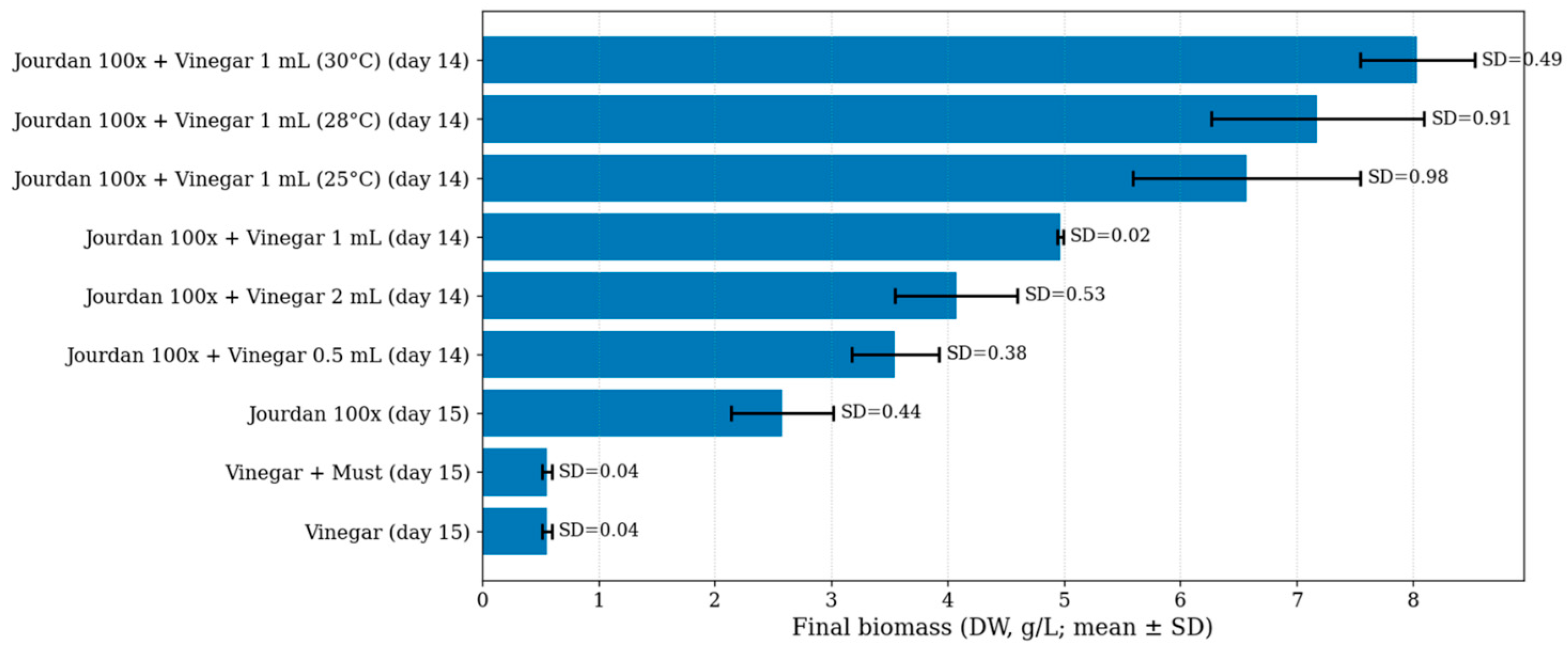
Across the acidic controls, biomass remained low throughout the campaign, consistent with the persistently acidic/weakly acidic pH. In contrast, Jourdan-based cultures exhibited a progressive biomass increase during the first week, followed by a stronger divergence in the second week. Vinegar dosage produced differentiated outcomes at day 14, with the 0.5 mL condition yielding a moderate improvement over the reference, the 2 mL condition showing intermediate performance, and the 1 mL condition reaching higher biomass values.
Temperature control further amplified productivity: the 25–30 °C trials produced the strongest end-point biomass, with a clear ranking across temperatures. Regarding culture chemistry, Jourdan-based experiments remained alkaline overall but showed a marked pH depression around the mid-campaign (≈days 8–9) followed by recovery, whereas the vinegar(-must) controls remained stably acidic. Together, these contrasted trends highlight the combined role of dosing and thermal regime in modulating Jourdan-based mixotrophic cultivation outcomes (detailed DW and pH time-course data are provided in Supplementary Figure S2).
The contrasted behaviour observed in Figure 1 and Figure 2 is consistent with the broader Limnospira/Arthrospira literature, which identifies medium composition, pH control, and cultivation regime as major determinants of biomass productivity. Recent studies have shown that non-conventional water resources can support Arthrospira growth, but performance remains strongly dependent on the physicochemical characteristics of the medium [32]. Likewise, pH modulation has been shown to directly affect biomass productivity and bioactive-compound synthesis in L. platensis, confirming the central role of culture chemistry in shaping biomass trajectories [33]. In this light, the poor performance observed in the vinegar-only and vinegar–must conditions should not be interpreted as evidence that vinegar-derived streams are intrinsically unsuitable for algal systems. Rather, under the present L. platensis monoculture conditions, the resulting pH regime and medium balance remained less favorable for sustained biomass accumulation. This interpretation is consistent with previous work showing that vinegar-processing wastewater may support biomass generation in other algal systems [7], while mixotrophic or supplemented cultivation strategies can enhance growth only when the underlying physiological requirements of the culture are preserved [4].
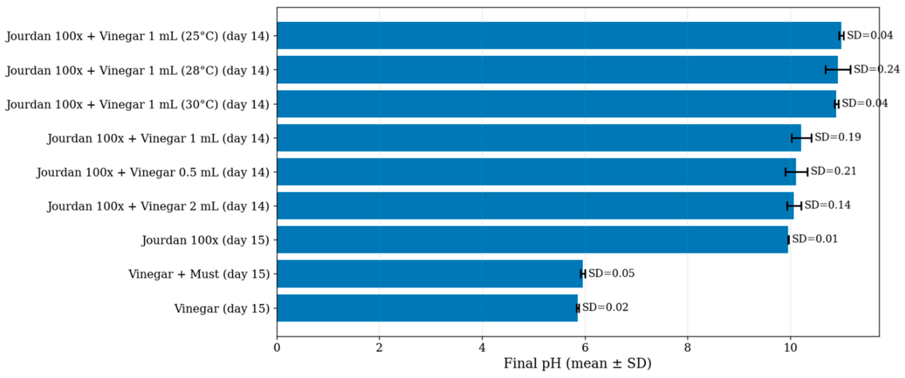
To synthesize the overall outcome across experiments, the final DW values highlight a clear contrast between Jourdan-based trials (robust biomass accumulation) and the vinegar-based culture-liquid runs (V and VM), which remained at very low biomass. Reporting mean ± SD emphasizes that dispersion is not uniform across conditions and should be considered when comparing endpoints and when defining uncertainty bounds for subsequent modeling analyses (Figure 1).
Culture pH followed two distinct regimes: Jourdan-based cultivations remained predominantly alkaline with temporary mid-cultivation decreases followed by recovery, whereas vinegar-only and vinegar + must conditions stayed in a near-acidic/weakly acidic range. The final pH comparison provides a compact view of these differences and their variability at the endpoint (Figure 2).

3.2. Multi-Horizon DW Forecasting Performance

To better contextualize the machine-learning results, we refer to the logistic growth model as a simple mechanistic framework commonly used to describe biomass evolution under resource-limited conditions. In this formulation, biomass growth is represented as:
dX/dt = μmax·X·(1 − X/Xmax)
where X is biomass concentration, μmax is the maximum specific growth rate, and Xmax represents the carrying capacity. Although this model provides a biologically interpretable description of smooth growth trajectories, its fixed-parameter structure may be less suitable for the present experimental conditions, where biomass evolution is influenced by transient perturbations, pH shifts, substrate addition, and regime-dependent variability. Direct multi-step forecasting models were developed to predict L. platensis dry weight (DW) at horizons h = 1, 2, and 3 measurement steps ahead. Model development and evaluation were conducted under a Leave-One-Experiment-Out (LOEO) cross-validation framework to assess generalization to unseen cultivation runs. This grouped validation strategy is particularly appropriate for biological time series, where repeated measurements within the same experiment are strongly autocorrelated and cannot be considered statistically independent. The dataset comprised 9 independent experiments across 4 experimental conditions, covering a cultivation window of Day 0–15, with DW values ranging from approximately 0.13 to 8.04 g L−1 and pH values between 5.61 and 11.39. The relatively high OD680-to-DW coefficient used in this study deserves specific consideration. Although OD-to-DW factors of approximately 0.3–0.6 g L−1 per OD unit are often reported, this range should not be regarded as universal. OD-to-DW relationships depend on the strain, wavelength, instrument, optical pathlength, pigment content, filament morphology, physiological state, and dry-weight protocol. Importantly, OD680-to-DW slopes close to the value used here have been reported for Limnospira/Arthrospira platensis. For example, in a recent L. platensis study, an OD680–DW regression based on gravimetric biomass determination was used, reporting a biomass content = 1.037 × OD680, R2 = 0.9523 [34]. Furthermore, it has been reported that OD680–DW relationships in S. platensis can vary markedly with physiological adaptation, reporting 0.477 × OD680 + 0.376 for non-adapted cultures and 2.35 × OD680 + 0.32 for salinity-adapted cultures [35]. Together, these examples demonstrate that OD-to-DW coefficients are not universal constants and that values around or above 0.9 g L−1 per OD680 unit can be experimentally obtained under specific strain-, medium-, physiological-, and instrument-dependent conditions. From a biological perspective, a higher DW/OD680 ratio may occur when biomass contains a larger fraction of reserve compounds, such as carbohydrates or lipids, which contribute to dry mass but absorb less strongly at 680 nm than chlorophyll- and phycobiliprotein-associated pigments. In filamentous cyanobacteria, trichome length, coiling, aggregation, and optical package effects may also modify the relationship between dry mass and apparent absorbance. Therefore, the conversion factor used in this study is best interpreted as an experiment-specific calibration coefficient rather than a general property of L. platensis.
The highest biomass values observed in this study should be interpreted within the specific context of the adopted flask-scale cultivation system, characterized by a low working volume, short optical pathlength, improved light penetration, controlled aeration, LED illumination, and vinegar supplementation. Therefore, these OD-derived DW estimates should not be directly compared with biomass levels typically reported for larger-scale PBRs or outdoor systems, where self-shading, longer optical paths, hydrodynamic gradients, and mass-transfer limitations are more pronounced.
Cross-scale comparisons remain informative at the level of qualitative biological trends; however, direct transfer of a predictor trained on the present dataset to larger photobioreactor or outdoor systems would require external validation, because light gradients, hydrodynamics, gas transfer, and operational control can substantially modify the biomass dynamics captured by the model [8,12,36]. In this regard, while this dataset supports a robust evaluation of model performance under a leakage-safe validation framework, the relatively small number of independent experiments may limit the full generalizability of the predictive model to a wider range of cultivation conditions. A conservative rescaling of the OD-to-DW coefficient would modify the absolute biomass values and absolute error metrics, but would not alter the temporal patterns, treatment ranking, model comparison, or R2-based conclusions of the forecasting analysis. Finally, minor within-experiment duplicate day entries were present, corresponding to phase-specific measurements acquired on the same day, but no temporal inversions were detected, confirming the internal chronological consistency of the experimental records.
From a theoretical standpoint, the present forecasting problem is characterized by nonlinear and condition-dependent biomass dynamics, in which pH, nutrient availability, environmental history, and cultivation regime interact over time. This motivates the use of flexible data-driven models alongside simple mechanistic references. Recent contributions on microalgal cultivation systems have highlighted that dynamic and data-driven approaches are particularly valuable when growth trajectories deviate from smooth, fixed-parameter behaviour because of transient physicochemical perturbations or heterogeneous operating conditions [9,10,20]. In parallel, reactor-scale studies emphasize that light distribution, hydrodynamics, and process control can substantially influence biomass evolution across cultivation systems [8,12,36]. For this reason, the present results are discussed in terms of biological consistency and predictive robustness, while avoiding any assumption of direct quantitative transferability beyond the experimental domain covered by the dataset.
Therefore, the high LOEO R2 values reported here demonstrate robust interpolation across the available flask-scale experiments, but they should not be read as evidence of direct quantitative transferability to pilot or industrial cultivation. In larger systems, scale-dependent transport phenomena may change biomass-pH relationships and invalidate lagged-biomass features learned under well-mixed, short-optical-path flask conditions. The model is therefore most appropriately viewed as a transferable workflow—rather than a directly transferable parameter set—for future datasets generated under larger photobioreactor configurations [23,24,25,26].
Horizon h = 1: one-step-ahead forecasting (Figure 3a–c)
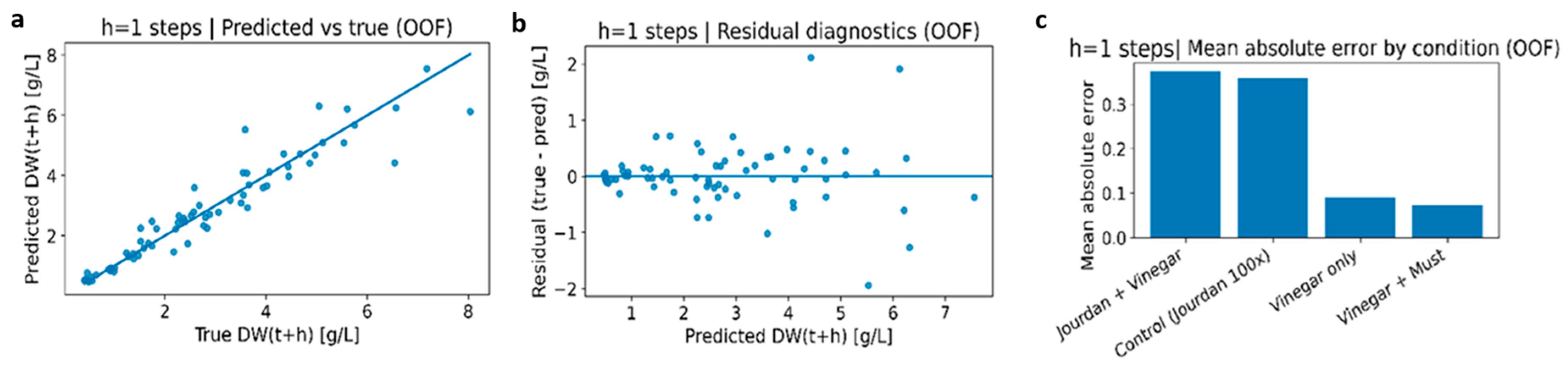
At the shortest forecasting horizon (h = 1), Gradient Boosting exhibited the strongest predictive performance among the evaluated models and substantially outperformed the persistence (naïve) baseline. Out-of-fold evaluation yielded R2 = 0.9149, RMSE = 0.5356 g L−1, and MAE = 0.3256 g L−1 for Gradient Boosting, compared with R2 = 0.7283, RMSE = 0.9574 g L−1, and MAE = 0.6624 g L−1 for persistence. The predicted-versus-observed scatter plot (Figure 3a) shows a pronounced alignment of predictions with the identity line across most of the DW range, indicating that the model effectively captures short-term biomass dynamics when trained on heterogeneous experiments and evaluated on a fully unseen run. Residual diagnostics (Figure 3b) reveal residuals centered around zero with no evident systematic bias, supporting the adequacy of the mean prediction. However, residual dispersion increases moderately at higher predicted DW values, suggesting mild heteroscedasticity even at the one-step horizon. This behavior is biologically plausible, as later growth phases often involve increased sensitivity to nutrient availability, light attenuation, and physiological stress, which can amplify variability in biomass accumulation.
Condition-level error stratification (Figure 3c) highlights non-uniform predictive difficulty across cultivation regimes. Jourdan-based conditions, including both control and vinegar-supplemented variants, exhibit higher MAE values than vinegar-based conditions. In contrast, “Vinegar only” and “Vinegar + must” conditions show lower absolute errors, albeit with fewer available samples, which may limit the stability of their aggregated statistics.
Further detail is provided in Supplementary Figure S3.
Horizon h = 2: two-step-ahead forecasting (Figure 4a–c)
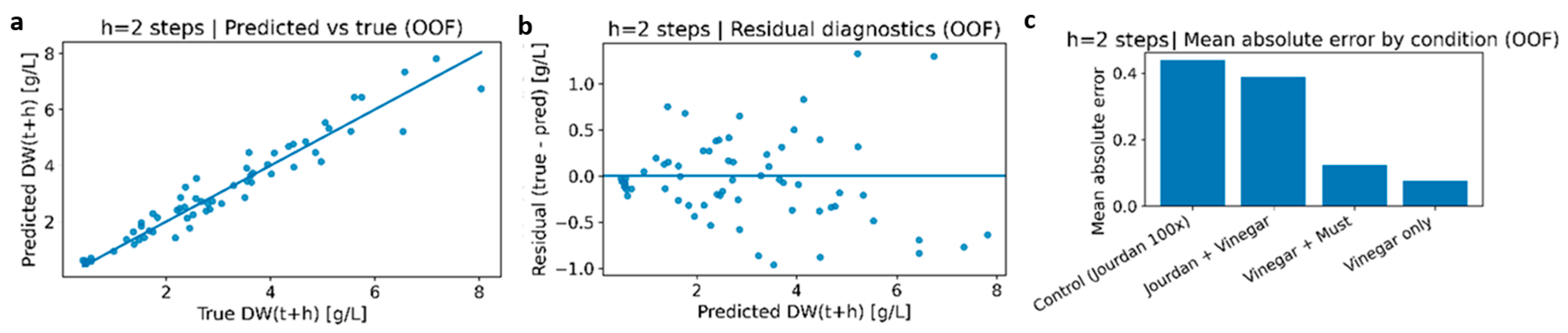
At the intermediate horizon (h = 2), predictive performance remained strong and the advantage over the persistence baseline became more pronounced. Gradient Boosting achieved R2 = 0.9353, RMSE = 0.4623 g L−1, and MAE = 0.3490 g L−1, while persistence performance degraded substantially to R2 = 0.4601, RMSE = 1.3354 g L−1, and MAE = 1.0459 g L−1. The predicted-versus-observed scatter (Figure 4a) continues to show a tight clustering around the identity line, indicating that the direct multi-step formulation preserves accuracy even when forecasting two measurement steps ahead. Residuals at this horizon (Figure 4b) remain broadly centered around zero, confirming the absence of systematic bias. Nonetheless, dispersion increases relative to h = 1, particularly at higher predicted DW values, indicating that uncertainty accumulation becomes more pronounced as the forecast step increases. This trend is consistent with the compounding effect of biological variability and unmodeled environmental perturbations over longer prediction intervals.
Condition-level MAE profiles (Figure 4c) largely reproduce the regime-dependent patterns observed at h = 1, with Jourdan-based conditions remaining more challenging to predict than vinegar-based regimes.
Further detail is provided in Supplementary Figure S4.
Horizon h = 3: three-step-ahead forecasting (Figure 5a–c)
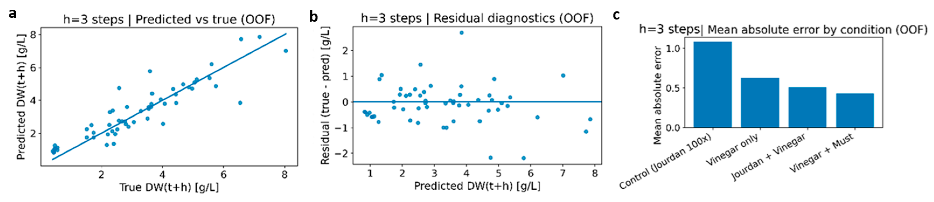
At the longest horizon (h = 3), predictive performance decreased as expected but remained substantially superior to the baseline. Gradient Boosting achieved R2 = 0.8143, RMSE = 0.7769 g L−1, and MAE = 0.5516 g L−1, whereas persistence performance collapsed to R2 = 0.1136, RMSE = 1.6973 g L−1, and MAE = 1.3573 g L−1. The predicted-versus-observed relationship (Figure 5a) retains a clear monotonic trend, though with visibly increased dispersion compared to shorter horizons, reflecting the growing difficulty of anticipating biomass trajectories several steps in advance. Residual diagnostics (Figure 5b) show a broader spread and more pronounced outliers, supporting the interpretation that a subset of experiments undergoes transitions, such as abrupt growth acceleration or deceleration, that are inherently difficult to anticipate at longer horizons. Condition-level stratification (Figure 5c) continues to reveal higher errors in Jourdan-based regimes, while vinegar-based conditions remain comparatively easier to predict, again acknowledging the influence of sample-size imbalance.
Further detail is provided in Supplementary Figure S5.
Cross-horizon comparison and implications
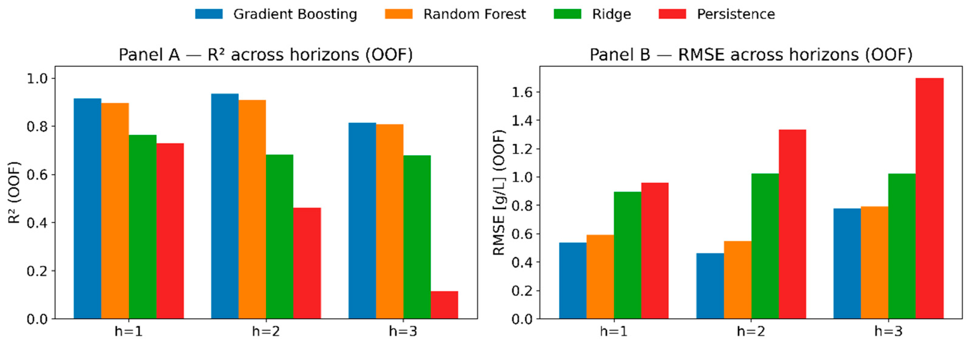
Comparing horizons, Gradient Boosting consistently delivered the highest predictive accuracy and robustly outperformed persistence across all forecast steps (Table 2). The persistence baseline exhibited rapid degradation with horizon, with R2 declining from approximately 0.73 at h = 1 to 0.11 at h = 3, underscoring the inadequacy of naïve extrapolation for medium-term biomass forecasting. Random Forest remained competitive but consistently inferior to Gradient Boosting (R2 = 0.8957/0.9088/0.8075 for h = 1/2/3), while Ridge regression performed substantially worse, particularly in relative-error metrics, indicating that nonlinear learners are better suited to capture the condition-dependent growth dynamics present in these cultivation data.
The performance patterns reported in Table 2 and Figure 3, Figure 4, Figure 5 and Figure 6 are also coherent with the current literature on predictive modeling in microalgal systems. Reviews and recent studies consistently show that nonlinear learners are generally better suited than linear baselines to represent biomass dynamics governed by interacting environmental and operational drivers [20,36,37]. This provides a theoretical basis for the inferior performance of Ridge regression in the present study. Likewise, the advantage of Gradient Boosting over the persistence baseline is consistent with previous evidence that structured feature engineering and boosting-based models can effectively exploit short-term temporal memory and condition-dependent interactions in Limnospira and related microalgal datasets [17,18]. The progressive loss of accuracy from h = 1 to h = 3 is also expected in biological time-series forecasting, because uncertainty accumulates with prediction horizon and unmodeled perturbations become increasingly relevant over longer intervals [9,10,20]. Finally, the use of Leave-One-Experiment-Out validation directly addresses a key concern raised in the literature, namely that models assessed on temporally correlated samples from the same cultivation run may overestimate generalization and perform poorly on unseen experiments or batches [17,20].
Across all horizons, residual patterns indicate mild heteroscedasticity at higher DW values and regime-dependent predictability limits, while prediction intervals remain close to nominal coverage and expand with horizon in a manner consistent with observed error growth. This reduced predictability can be interpreted in light of the underlying biological and physicochemical dynamics of the system. Jourdan-based media are typically associated with greater variability in pH and nutrient availability, which can induce non-linear and transient responses in Limnospira growth. Fluctuations in pH influence inorganic carbon speciation and uptake efficiency, while nutrient imbalances may trigger stress responses and alter metabolic activity. These effects can lead to deviations from smooth growth trajectories, making it more difficult for data-driven models to capture consistent patterns. In contrast, more controlled or supplemented conditions may provide more stable environments, resulting in more predictable biomass dynamics. The limitations of mechanistic models such as the logistic equation further support this interpretation. While these models assume smooth and continuous growth trajectories, the experimental data exhibit regime shifts and transient dynamics that violate these assumptions. In particular, abrupt changes in pH and nutrient availability introduce non-stationary behavior that cannot be captured by fixed-parameter kinetic models.
In contrast, machine learning models are able to adapt to such nonlinear and condition-dependent patterns, which explains their superior predictive performance observed in this study.
Collectively, the evidence from Figure 3, Figure 4 and Figure 5 (panels a–c) demonstrates that direct multi-step forecasting under LOEO validation provides reliable biomass predictions while transparently revealing the experimental regimes and conditions that constitute the primary sources of remaining uncertainty.
Figure 6 provides a concise overview of how forecasting horizon affects model performance under Leave-One-Experiment-Out validation. Gradient Boosting consistently achieves the highest accuracy across all horizons, with strong performance at h = 1–2 (R2 = 0.915–0.935) and a more moderate decline at h = 3 (R2 = 0.814), indicating robust inter-experiment generalization as uncertainty increases. Random Forest follows a similar trend but remains systematically inferior, suggesting that the bias–variance trade-off achieved by boosting is more effective at capturing the nonlinear, condition-dependent growth dynamics. As the horizon increases, the persistence baseline degrades sharply, with both declining R2 and increasing RMSE, demonstrating that naïve extrapolation of the last observed value is inadequate for medium-term biomass forecasting. Ridge regression shows consistently weaker performance and a more pronounced deterioration relative to nonlinear models, supporting the notion that linear approaches struggle to represent regime-dependent and nonlinear growth behavior.
Overall, the combined trends in R2 (Panel A) and RMSE (Panel B) confirm the expected growth of prediction error with horizon, while highlighting that direct multi-step forecasting with Gradient Boosting retains reliable predictive skill and represents the most robust option for operational biomass prediction. These results contribute to the growing body of evidence on machine learning applications in algal cultivation systems, recently reviewed in the context of biofuel production and bioprocess optimization [37,38]. In this perspective, future hybrid or digital-twin-oriented frameworks may benefit from integrating data-driven prediction with regime-aware monitoring and mechanistic process knowledge.

3.3. Model Interpretability and Feature Importance

To improve the interpretability of the predictive framework, the model-based feature importance for the selected Gradient Boosting models at each forecasting horizon was examined. Across all horizons, biomass-history variables were the dominant predictors, indicating that short-term biomass forecasts were driven primarily by the recent state of the culture.
At h = 1, the most influential feature was DW_lag1 (66.1%), followed by DW_t (10.3%), DW_roll3_t (9.8%), and DW_lag2 (6.2%). At h = 2, DW_t became the dominant predictor (72.5%), with additional contributions from DW_lag1 (8.4%), DW_lag2 (5.0%), and pH_mean (5.0%). At h = 3, DW_t remained the leading predictor (62.2%), while the relative importance of pH_mean increased (13.2%), followed by DW_lag1 (8.3%) and DW_diff_t (5.6%).
When grouped by feature family, biomass-history variables accounted for approximately 94.0%, 92.1%, and 83.0% of the total importance at h = 1, h = 2, and h = 3, respectively, whereas pH-related variables increased from 5.3% to 13.8% as the forecasting horizon lengthened. This pattern is biologically plausible: near-term biomass forecasts depend mainly on recent biomass memory, whereas longer-horizon predictions are more sensitive to culture chemistry, particularly pH dynamics, which affect inorganic carbon availability and metabolic activity.
These importance patterns are consistent with the experimental behaviour discussed above. In particular, the increasing contribution of pH-related variables at longer forecasting horizons suggests that, as the prediction step extends, biomass evolution is influenced not only by recent biomass history but also more strongly by changes in culture chemistry.

4. Conclusions

This study demonstrated the feasibility of applying machine learning techniques to predict biomass (DW, g L−1) accumulation in L. platensis cultures under different nutritional conditions. A direct multi-step forecasting framework based on Gradient Boosting regression was developed and rigorously validated using a leakage-resistant methodology with leave-one-experiment-out cross-validation.
The proposed model achieved substantial predictive performance across all forecasting horizons, with out-of-fold R2 values of 0.915, 0.935, and 0.814 for one-, two-, and three-step-ahead predictions, respectively. These results represent a marked improvement over the persistence baseline, with R2 gains ranging from +0.19 to +0.70 depending on the horizon. The statistical significance of the predictive signal was confirmed through permutation testing (p < 0.01), ruling out the possibility that the observed performance arose from spurious correlations or data leakage.
The analysis revealed that prediction accuracy varied across experimental conditions, with vinegar-supplemented Jourdan medium cultures exhibiting higher prediction errors compared to control and vinegar-only treatments. This finding suggests that the metabolic response to combined nutritional inputs introduces additional variability that warrants further investigation with larger sample sizes. In this context, it is important to note that the present study is based on a limited number of independent experiments (n = 9), which may constrain the generalizability of the proposed model across a broader range of cultivation conditions. Although the adoption of leakage-safe validation strategies ensures robust performance assessment within the available dataset, further improvements in model reliability and transferability will require expanding the experimental space. In particular, future studies should include additional cultivation trials under diverse operational conditions and potentially different Limnospira strains to better capture variability in growth dynamics and enhance model scalability.
Several limitations should be acknowledged. The dataset comprised nine experiments with approximately 6–8 usable samples per experiment after feature construction, which constrains the generalizability of the findings. Additionally, the forecasting horizons correspond to measurement steps rather than fixed temporal intervals, reflecting the irregular sampling schedule inherent to the experimental design. Future work should validate these results on independent datasets and explore the integration of mechanistic and data-driven approaches. At the same time, the applicability of models trained on flask-scale data to industrial PBRs should not be assumed a priori, since differences in optical path, light gradients, hydrodynamics, mixing, and operational control may substantially modify biomass dynamics and the relationships learned from the present dataset. In particular, hybrid modeling frameworks combining interpretable kinetic models (e.g., logistic or Monod-type formulations) with machine learning could improve both predictive accuracy and biological interpretability.
A practical scale-up pathway would therefore require staged validation: (1) additional flask experiments to enlarge the biological and nutritional design space, (2) intermediate bench- or pilot-scale photobioreactor trials to quantify light, mixing, and gas-transfer effects, and (3) prospective external testing in which predictions are generated before biomass measurements are available. Such a sequence would allow the same leakage-safe pipeline to be progressively transferred from proof-of-concept forecasting to operational decision support while explicitly controlling for scaling effects [23,24,25,26].
Despite these limitations, the present work establishes a methodological foundation for data-driven growth prediction in cyanobacterial cultivation systems. Although the present study is based on a limited number of independent experiments (n = 9), the proposed modeling workflow is methodologically scalable, but the trained model itself should be considered scale-specific until validated on independent photobioreactor and outdoor datasets. Expanding the dataset to include additional cultivation trials, diverse operational conditions, and different Limnospira strains represents a key step toward improving model generalizability and enabling its application in real-world and industrial settings. The demonstrated ability to forecast biomass accumulation multiple sampling steps ahead has practical implications for process optimization, including reduced sampling frequency and improved feed-forward control strategies in PBR operation. The complete analytical pipeline, including bootstrap confidence intervals, prediction intervals with empirical coverage validation, and per-experiment stability indices, provides a reproducible template for future studies in algal biotechnology.

Supplementary Materials

The following supporting information can be downloaded at: https://www.mdpi.com/article/10.3390/biomass6030041/s1, the Supplementary File includes Figure S1, photographic overview of the flask-scale cultivation setup; Figure S2, DW and pH time-course data across the experimental conditions; and Figures S3–S5, additional forecasting diagnostics for h = 1–3.

Author Contributions

Conceptualization, B.C., G.A.L. and G.C.; Methodology, B.C., G.A.L., A.C. (Alida Cosenza), A.C. (Alessandro Concas), G.C., C.V.P. and L.U.; Software, B.C.; Validation, B.C., A.C. (Alessandro Concas), C.V.P. and M.P.; Formal analysis, B.C., G.A.L., L.U. and M.P.; Investigation, B.C., G.A.L., L.U., M.P. and A.C. (Alida Cosenza); Resources, G.A.L. and B.C.; Data curation, B.C., G.A.L., C.V.P. and M.P.; Writing—original draft preparation, B.C.; Writing—review and editing, B.C., G.A.L., A.C. (Alessandro Concas), G.C., A.C. (Alida Cosenza) and C.V.P.; Visualization, B.C., G.A.L., A.C. (Alida Cosenza) and L.U.; Supervision, B.C., A.C. (Alessandro Concas), G.A.L. and G.C. All authors have read and agreed to the published version of the manuscript.

Funding

Part of the project was funded under the National Recovery and Resilience Plan (NRRP), Mission 4 Component 2 Investment 1.3—Call for tender No. 1561 of 11.10.2022 of Ministero dell’Università e della Ricerca (MUR); funded by the European Union—NextGenerationEU: Award Number: Project code PE0000021, Concession Decree No. 1561 of 11.10.2022 adopted by Ministero dell’Università e della Ricerca (MUR), CUP—I53C22001450006, Project title “Network 4 Energy Sustainable Transition—NEST”.

Data Availability Statement

Data are available from the corresponding author upon reasonable request. The dataset originates from experimental activities conducted in collaboration with an industrial partner (Teregroup Srl) and is therefore subject to confidentiality constraints. However, access may be granted to academic researchers for non-commercial purposes, subject to approval by the data owner and appropriate data-sharing agreements.

Acknowledgments

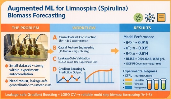
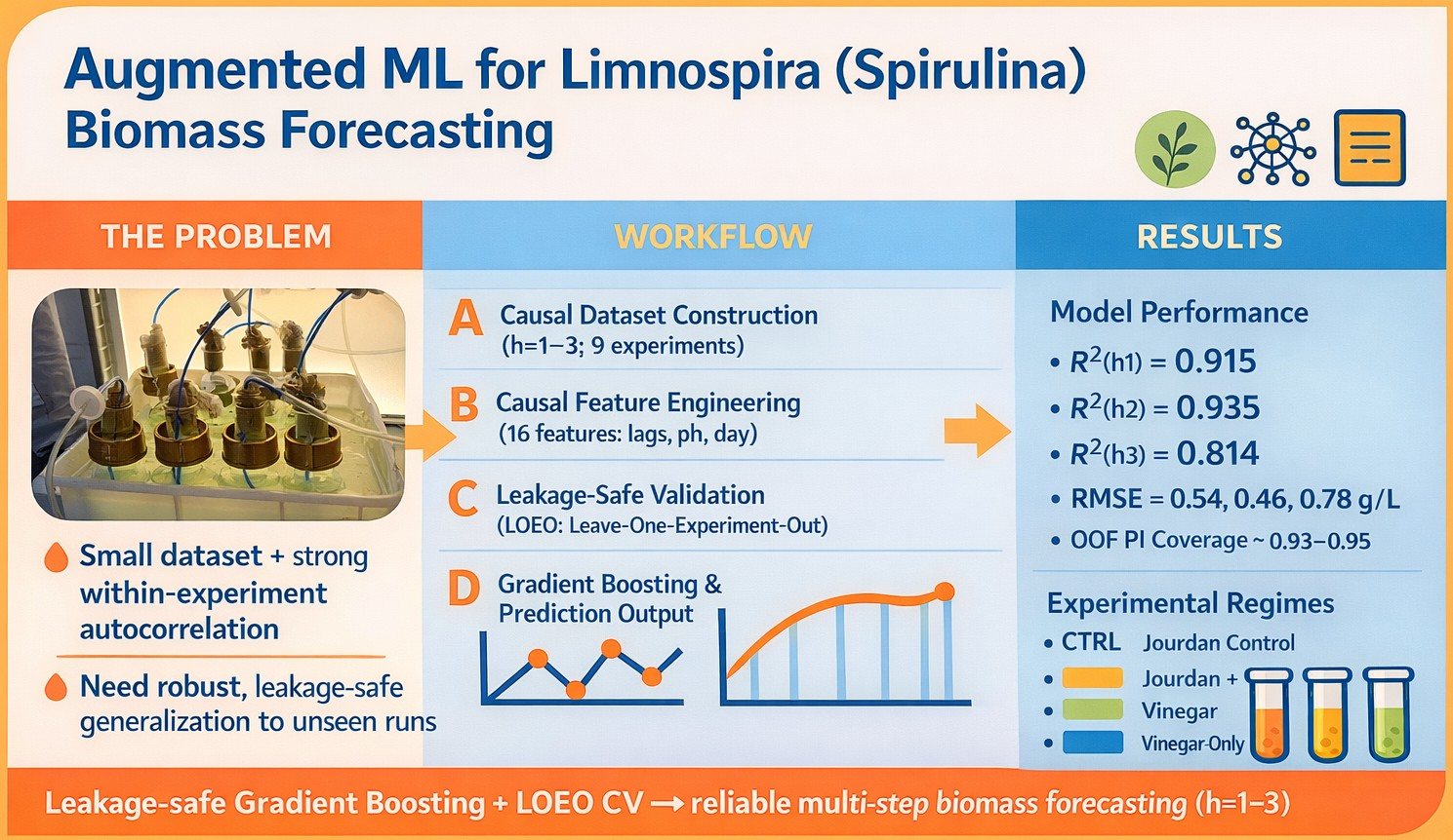
During the preparation of this work, the authors used Claude (Sonnet 4.5, Anthropic) to re-phrase selected paragraphs with the sole aim of improving the manuscript’s fluency and readability, and ChatGPT (GPT-5.1, OpenAI) to provide partial support in generating the graphical abstract. After using these tools, the authors reviewed and edited the content as needed and take full responsibility for the content of the manuscript.

Conflicts of Interest

The authors declare no conflicts of interest. Dr. Luca Usai and Dr. Giovanni Antonio Lutzu are affiliated with Teregroup Srl (Modena, Italy), which provided the experimental data used in this study. The authors are solely responsible for the analysis, interpretation, and reporting of the results.

Abbreviations

The following abbreviations are used in this manuscript:
DWDry Weight
GBGradient Boosting
LOEOLeave-One-Experiment-Out
MAEMean Absolute Error
MAPE Mean Absolute Percentage Error
OOFOut-of-Fold
PBRPhotobioreactor
PIPrediction Interval
RFRandom Forest
RMSERoot Mean Squared Error
SDStandard Deviation
JMJourdan 100× medium
VVinegar
VMvinegar–must stream
ODoptical density (OD-based procedure, OD at 680 nm)
PARphotosynthetically active radiation
PVDFpolyvinylidene fluoride
UV–Visultraviolet–visible

References

  1. Sinetova, M.; Kupriyanova, E.; Los, D. Spirulina/Arthrospira/Limnospira—Three Names of the Single Organism. Foods 2024, 13, 2762. [Google Scholar] [CrossRef] [Scilit]
  2. Roussel, T.; Halary, S.; Duval, C.; Piquet, B.; Cadoret, J.-P.; Vernès, L.; Bernard, C.; Marie, B. Monospecific renaming within the cyanobacterial genus Limnospira (Spirulina) and consequences for food authorization. J. Appl. Microbiol. 2023, 134, lxad159. [Google Scholar] [CrossRef] [Scilit]
  3. Lutzu, G.A.; Marin, M.A.; Concas, A.; Dunford, N.T. Growing Picochlorum oklahomensis in hydraulic fracking wastewater supplemented with animal wastewater. Water Air Soil Pollut. 2020, 231, 457. [Google Scholar] [CrossRef] [Scilit]
  4. Russo, N.P.; Ballotta, M.; Usai, L.; Torre, S.; Giordano, M.; Fais, G.; Casula, M.; Dessì, D.; Nieri, P.; Damergi, E.; et al. Mixotrophic Cultivation of Arthrospira platensis (Spirulina) under Salt Stress: Effect on Biomass Composition, FAME Profile and Phycocyanin Content. Mar. Drugs 2024, 22, 381. [Google Scholar] [CrossRef] [Scilit]
  5. Cosenza, A.; Lima, S.; Gurreri, L.; Mancini, G.; Scargiali, F. Microalgae in the Mediterranean Area: A Geographical Survey Outlining the Diversity and Technological Potential. Algal Res. 2024, 82, 103669. [Google Scholar] [CrossRef] [Scilit]
  6. Franzoso, L.; Usai, L.; Allodi, R.; Fais, G.; Dessì, D.; Soto-Ramirez, R.; Cosenza, B.; Damergi, A.; Lutzu, G.A.; Concas, A. Mixotrophic Cultivation of Limnospira (Spirulina) platensis Using Early-Stage Fig Processing Wastewater: Effects on Biomass Composition, Antioxidants and Phycocyanin. Mar. Drugs 2026, 24, 163. [Google Scholar] [CrossRef] [Scilit] [PubMed]
  7. Huo, S.; Kong, M.; Zhu, F.; Qian, J.; Huang, D.; Chen, P.; Ruan, R. Co-Culture of Chlorella and Wastewater-Borne Bacteria in Vinegar Production Wastewater: Enhancement of Nutrients Removal and Influence of Algal Biomass Generation. Algal Res. 2020, 45, 101744. [Google Scholar] [CrossRef] [Scilit]
  8. Ma, G.; Gao, Q.; Yuan, L.; Chen, Y.; Cai, Z.; Zhang, L.; Hu, J.; Wang, Y.; Wu, S.; Sun, Y. Spirulina (Arthrospira) Cultivation in Photobioreactors: From Biochemistry and Physiology to Scale-Up Engineering. Bioresour. Technol. 2025, 423, 132259. [Google Scholar] [CrossRef] [Scilit] [PubMed]
  9. Galang, M.G.K.; Chen, J.; Cobb, K.; Zarra, T.; Ruan, R. Intelligent Predictive Modeling for the Optimization of Advanced Algal Photobioreactors in Greenhouse Gas Capture and Utilization. J. Environ. Manag. 2025, 381, 125275. [Google Scholar] [CrossRef] [Scilit] [PubMed]
  10. Aowtrakool, N.; Sopitthummakhun, A.; Laomettachit, T.; Ruengjitchatchawalya, M. A Dynamic Model for Predicting Biomass and Phycocyanin Yields in Arthrospira (Spirulina) platensis: A Guidance for Effective Batch Cultivation. Algal Res. 2024, 83, 103709. [Google Scholar] [CrossRef] [Scilit]
  11. Leca, M.A.; Beigbeder, J.B.; Castel, L.; Sambusiti, C.; Le Guer, Y.; Monlau, F. Cultivation of Arthrospira platensis Using Different Agro-Industrial Liquid Anaerobic Digestates Diluted with Geothermal Water: A Sustainable Culture Strategy. Algal Res. 2024, 77, 103348. [Google Scholar] [CrossRef] [Scilit]
  12. Amanna, B.; Bahri, P.A.; Moheimani, N.R. Application of Computational Fluid Dynamics in Optimizing Microalgal Photobioreactors. Algal Res. 2024, 83, 103718. [Google Scholar] [CrossRef] [Scilit]
  13. Altriki, A.; Ali, I.; Razzak, S.A.; Ahmad, I.; Farooq, W. Assessment of CO2 Biofixation and Bioenergy Potential of Microalga Gonium pectorale through Biomass Pyrolysis, and Elucidation of Pyrolysis Reaction via Kinetics Modeling and Artificial Neural Network. Front. Bioeng. Biotechnol. 2022, 10, 925391. [Google Scholar] [CrossRef] [Scilit] [PubMed]
  14. Hossain, S.Z.; Sultana, N.; Razzak, S.A.; Hossain, M.M. Modeling and Multi-Objective Optimization of Microalgae Biomass Production and CO2 Biofixation Using Hybrid Intelligence Approaches. Renew. Sustain. Energy Rev. 2022, 157, 112016. [Google Scholar] [CrossRef] [Scilit]
  15. Singh, V.; Verma, M.; Chivate, M.S.; Mishra, V. Machine Learning-Based Optimisation of Microalgae Biomass Production by Using Wastewater. J. Environ. Chem. Eng. 2023, 11, 111387. [Google Scholar] [CrossRef] [Scilit]
  16. Kumar, R.R.; Sarkar, D.; Sen, R. Simultaneously Maximizing Microalgal Biomass and Lipid Productivities by Machine Learning-Driven Modeling, Global Sensitivity Analysis and Multi-Objective Optimization for Sustainable Biodiesel Production. Appl. Energy 2024, 358, 122597. [Google Scholar] [CrossRef] [Scilit]
  17. Cosenza, B.; Allodi, R.; Usai, L.; Minardi, R.; Cosenza, A.; Soto-Ramirez, R.; Concas, A.; Lutzu, G.A. Advanced Feature Engineering and Gradient Boosting Optimization for Predicting Limnospira platensis Growth Dynamics under Mixotrophic Conditions Using Agro-Industrial Byproducts. Algal Res. 2025, 93, 104445. [Google Scholar] [CrossRef] [Scilit]
  18. Yeh, Y.C.; Syed, T.; Brinitzer, G.; Frick, K.; Schmid-Staiger, U.; Haasdonk, B.; Tovar, G.E.M.; Krujatz, F.; Mädler, J.; Urbas, L. Improving Microalgae Growth Modeling of Outdoor Cultivation with Light History Data Using Machine Learning Models: A Comparative Study. Bioresour. Technol. 2023, 390, 129882. [Google Scholar] [CrossRef] [Scilit] [PubMed]
  19. Santos, J.M.; Zelioli, I.A.M.; Guimaraes, E.E.X.; Freitas, A.C.D.; Mariano, A.P. Supercritical Water Gasification Thermodynamic Study and Hybrid Modeling of Machine Learning with the Ideal Gas Model: Application to Gasification of Microalgae Biomass. Energy 2024, 291, 130287. [Google Scholar] [CrossRef] [Scilit]
  20. Syed, T.; Krujatz, F.; Ihadjadene, Y.; Mühlstädt, G.; Hamedi, H.; Mädler, J.; Urbas, L. A Review on Machine Learning Approaches for Microalgae Cultivation Systems. Comput. Biol. Med. 2024, 172, 108248. [Google Scholar] [CrossRef] [Scilit]
  21. Al-Huqail, A.; Mohammed, K.J.; Suhatril, M.; Almujibah, H.; Toghroli, S.; Alnahdi, S.S.; Ponnore, J.J. Optimizing Microalgal Biomass Conversion into Carbon Materials and Their Application in Water Treatment: A Machine Learning Approach. Carbon Lett. 2025, 35, 861–880. [Google Scholar] [CrossRef] [Scilit]
  22. Fu, Y.; Zhang, Q.; Tan, Z.; Yu, S.; Zhang, Y. Predicting Harvesting Efficiency of Microalgae with Magnetic Nanoparticles Using Machine Learning Models. J. Environ. Chem. Eng. 2025, 13, 115406. [Google Scholar] [CrossRef] [Scilit]
  23. Jin, M.; Xu, Y.; Chen, J.; Wei, X.; Yu, G.; Feng, M.; Cao, W.; Guo, L. A comprehensive universal model framework of microalgae growth dynamics for photobioreactor scaling-up design and optimization. Energy Convers. Manag. 2024, 299, 117832. [Google Scholar] [CrossRef] [Scilit]
  24. Hajinajaf, N.; Fallahi, A.; Eustance, E.; Sarnaik, A.; Askari, A.; Najafi, M.; Davis, R.W.; Rittmann, B.E.; Varman, A.M. Managing carbon dioxide mass transfer in photobioreactors for enhancing microalgal biomass productivity. Algal Res. 2024, 80, 103506. [Google Scholar] [CrossRef] [Scilit]
  25. Kumar, M.; Brar, A.; Kumari, R.; Vivekanand, V.; Pareek, N. Advancements in photobioreactor designs for development of microalgal biorefinery toward integrated remediation of industrial wastewater and product recovery. 3 Biotech 2025, 15, 274. [Google Scholar] [CrossRef] [Scilit]
  26. Wu, Y.; Shan, L.; Zhao, W.; Lu, X. Harnessing Artificial Intelligence to Revolutionize Microalgae Biotechnology: Unlocking Sustainable Solutions for High-Value Compounds and Carbon Neutrality. Mar. Drugs 2025, 23, 184. [Google Scholar] [CrossRef] [Scilit]
  27. Breiman, L.; Friedman, J.H.; Olshen, R.A.; Stone, C.J. Classification and Regression Trees; Chapman & Hall: New York, NY, USA, 1984. [Google Scholar]
  28. Friedman, J.H. Greedy Function Approximation: A Gradient Boosting Machine. Ann. Stat. 2001, 29, 1189–1232. [Google Scholar] [CrossRef] [Scilit]
  29. Chen, T.; Guestrin, C. XGBoost: A Scalable Tree Boosting System. In Proceedings of the 22nd ACM SIGKDD International Conference on Knowledge Discovery and Data Mining; Association for Computing Machinery: New York, NY, USA, 2016; pp. 785–794. [Google Scholar] [CrossRef] [Scilit]
  30. Anyanwu, R.C.; Rodriguez, C.; Durrant, A.; Olabi, A.G. Evaluation of Growth Rate and Biomass Productivity of Scenedesmus quadricauda and Chlorella vulgaris under Different LED Wavelengths and Photoperiods. Sustainability 2022, 14, 6108. [Google Scholar] [CrossRef] [Scilit]
  31. Trenkenshu, R.P. Calculation of the Specific Growth Rate of Microalgae. Mar. Biol. J. 2019, 4, 100–108. [Google Scholar] [CrossRef] [Scilit]
  32. Ansari, F.A.; Hassan, H.; Mahmud, U.; Rawat, I.; Bux, F. Cultivation of Arthrospira platensis in Non-Conventional Water Resources: A Comparative Analysis of Biomass Productivity and Chemical Constituents. Biomass Bioenergy 2025, 202, 108163. [Google Scholar] [CrossRef] [Scilit]
  33. Rizzoli, M.; Lutzu, G.A.; Usai, L.; Fais, G.; Dessì, D.; Soto-Ramirez, R.; Cosenza, B.; Concas, A. Photoautotrophic Batch Cultivation of Limnospira (Spirulina) platensis: Optimizing Biomass Productivity and Bioactive Compound Synthesis through Salinity and pH Modulation. Mar. Drugs 2025, 23, 281. [Google Scholar] [CrossRef] [Scilit]
  34. Baraldi, L.; Usai, L.; Torre, S.; Fais, G.; Casula, M.; Dessi, D.; Nieri, P.; Concas, A.; Lutzu, G.A. Dairy wastewaters to promote mixotrophic metabolism in Limnospira (Spirulina) platensis: Effect on biomass composition, phycocyanin content, and fatty acids methyl ester profile. Life 2025, 15, 184. [Google Scholar] [CrossRef] [Scilit]
  35. Ramirez-Perez, J.C.; Janes, H.W. Impact of salinity on the kinetics of CO2 fixation by Spirulina platensis cultivated in semi-continuous photobioreactors. Eclética Quím. J. 2021, 46, 21–34. [Google Scholar] [CrossRef] [Scilit]
  36. Razzak, S.A.; Bahar, K.; Islam, K.M.O.; Haniffa, A.K.; Faruque, M.O.; Hossain, S.M.Z.; Hossain, M.M. Microalgae cultivation in photobioreactors: Sustainable solutions for a greener future. Green Chem. Eng. 2024, 5, 418–439. [Google Scholar] [CrossRef] [Scilit]
  37. Meenatchisundaram, K.; Gowd, S.C.; Lee, J.; Barathi, S.; Rajendran, K. Data-Driven Model Development for Prediction and Optimization of Biomass Yield of Microalgae-Based Wastewater Treatment. Sustain. Energy Technol. Assess. 2024, 63, 103670. [Google Scholar] [CrossRef] [Scilit]
  38. Rayamajhi, V.; Hussain, M.; Shin, H.; Jung, S. Recent Advances in the Application of Artificial Intelligence in Microalgal Cultivation. Processes 2025, 13, 3764. [Google Scholar] [CrossRef] [Scilit]
Figure 1. Final dry weight (DW, g L−1) at the last sampling day for each experiment; bars show means and whiskers show SD.
Biomass 06 00041 g001
Figure 2. Final pH at the last sampling day for each experiment; bars show means and whiskers show SD.
Biomass 06 00041 g002
Figure 3. One-step-ahead forecasting (h = 1) under Leave-One-Experiment-Out (LOEO) cross-validation (out-of-fold predictions). Panels are ordered from left to right: (a) predicted vs. observed DW (identity line, y = x), (b) residuals (true − predicted) vs. predicted DW (zero line shown), (c) mean absolute error (MAE) by experimental condition. Blue points represent individual out-of-fold predictions.
Biomass 06 00041 g003
Figure 4. Two-step-ahead forecasting (h = 2) under Leave-One-Experiment-Out (LOEO) cross-validation (out-of-fold predictions). Panels are ordered from left to right: (a) predicted vs. observed DW (identity line, y = x), (b) residuals (true − predicted) vs. predicted DW (zero line shown), (c) mean absolute error (MAE) by experimental condition. Blue points represent individual out-of-fold predictions.
Biomass 06 00041 g004
Figure 5. Three-step-ahead forecasting (h = 3) under Leave-One-Experiment-Out (LOEO) cross-validation (out-of-fold predictions). Panels are ordered from left to right: (a) predicted vs. observed DW (identity line, y = x), (b) residuals (true − predicted) vs. predicted DW (zero line shown), (c) mean absolute error (MAE) by experimental condition. Blue points represent individual out-of-fold predictions.
Biomass 06 00041 g005
Figure 6. OOF (LOEO) performance for direct DW forecasts at h = 1–3: (A) R2 and (B) RMSE for Gradient Boosting, Random Forest, Ridge, and the persistence baseline.
Biomass 06 00041 g006
Table 1. Experimental workflow.
Experimental PhaseObjectiveCulture
Medium/Condition
Variable(s) TestedExperimental Structure
Phase I—Waste screeningAssess suitability of waste streams as sole culture mediaJM (control);
V;
VM
Type of culture liquid3 conditions × 4 replicates; ~2-week batch cultivation
Phase II—Mixotrophic stimulationEvaluate effect of organic carbon supplementation on established culturesJM + VVinegar dosage (0.5, 1, 2 mL per 150 mL culture)1 week photoautotrophic + 1-week mixotrophic; 3 conditions × 4 replicates
Phase III—Temperature × mixotrophyInvestigate interaction between temperature and mixotrophic growthJM + VTemperature values (25 °C, 28 °C, 30 °C) at fixed vinegar dose (1 mL per 150 mL culture)Temperature applied from day 0; mixotrophy induced at week 2 (vinegar addition); 3 conditions × 4 replicates
Table 2. Out-of-fold (Leave-One-Experiment-Out) performance across forecasting horizons (h = 1–3).
HorizonModelRMSE (g L−1)MAE (g L−1)R2MAPE (%)
1Gradient Boosting0.53560.32560.915012.98
1Random Forest0.59330.35930.895714.68
1Ridge0.89480.70700.762758.95
1Persistence0.95740.66240.728322.88
2Gradient Boosting0.46230.34900.935313.92
2Random Forest0.54880.39730.908818.89
2Ridge1.02650.84830.681067.79
2Persistence1.33541.04590.460133.26
3Gradient Boosting0.77690.55160.814330.59
3Random Forest0.79090.60880.807535.75
3Ridge1.02200.86680.678656.12
3Persistence1.69731.35730.113640.26
Disclaimer/Publisher’s Note: The statements, opinions and data contained in all publications are solely those of the individual author(s) and contributor(s) and not of MDPI and/or the editor(s). MDPI and/or the editor(s) disclaim responsibility for any injury to people or property resulting from any ideas, methods, instructions or products referred to in the content.