Abstract
This article describes systems generating high-frequency rotating magnetic fields for magnetic hyperthermia treatments. It covers two- and three-phase device systems powered by rectangular signals. A passive bandpass filter tuned to a specific frequency (100 kHz) is placed between the magnetic circuits and the DC power source powering the device. The paper compares the electrical parameters of both solutions, including the supply voltage, magnetic field strength amplitude H, and magnetizing current IL as a function of the supply voltage (Udc). At a fixed supply voltage Udc, the magnetizing current IL and the rotating magnetic field strength amplitude H are approximately twice as large for the three-phase system as for the two-phase system. The relationships between the magnetizing currents IL and the magnetic field strength amplitude H as a function of the supply voltage Udc are linear.
1. Introduction
High-frequency magnetic fields have been used in medicine to destroy oncological cells by heating tumors with a high-frequency magnetic field. For this purpose, magnetic nanoparticles (NP) are introduced into the tumor. According to the theory [1,2,3,4,5], magnetic nanoparticles (MNPs) under the influence of a variable external magnetic field become magnetized via two mechanisms, resulting in the release of thermal energy to the environment. The results of the Brownian mechanism and the Nèel mechanism depend on the hydrodynamic dh and magnetic dm size of the grain and on other physical quantities. These mechanisms are expressed by the formulas:
where τ0 = 1 ns is the characteristic time constant, K is the anisotropy constant, Vm is the volume of the MNP, k is the Boltzmann constant, T is the absolute temperature, VH is the hydrodynamic volume of the MNP and surfactant, and η is the dynamic viscosity of the carrier fluid. The relaxation mechanism with the shorter time constant dominates.
A characteristic feature of thermal energy losses in a magnetic fluid, as a result of magnetic relaxation, is the linear dependence of the volumetric power density P(f, H) on the square of amplitude H of the magnetic field intensity [1,5]:
where τ is the effective relaxation time, f is the operating frequency, μ0 is the magnetic permeability of vacuum, and χ″(f) is the imaginary component of magnetic susceptibility.
The imaginary component of magnetic susceptibility χ″(f) is a function of frequency f and the effective relaxation time τeff defined by the formula [1]:
If the value (2πfτ)2 << 1, then
To determine heating efficiency, two parameters are most often used: SLP and SAR [3,6,7,8].
The specific loss power (SLP) is defined as the thermal power dissipation divided by the mass of a magnetic material and can be expressed as [5,6]
where CP is the specific heat of the fluid (<10 mg/mL),
mS [mg] is the mass of the solvent,
mn [mg] is the mass of the nanoparticles.
The specific absorption rate (SAR) is defined as [5,6,9]
It should be added that SLP refers to the thermal power released in the magnetic material, while SAR refers to the thermal power released in the sample.
Very often MNPs show polydispersion, which means that in addition to superparamagnetic particles, there are also those with larger sizes in the sample. So there are also losses of thermal energy related to magnetic hysteresis, according to which the power of these losses P is proportional to f and to H3.
With patient safety in mind in clinical practice, special attention should also be paid to the permissible magnetic field parameters (H·f). There are several recommendations in the literature [3,7,10], including the Brezovich criterion, which states that the values of the H·f product obtained in therapeutic procedures will not be harmful to the patient when H·f < 4.85·108 A·m−1·s−1.
This means that at f = 100 kHz, the RMF intensity amplitude should not exceed 4.85 kA·m−1.
Slightly less stringent restrictions may also be found in the literature, with higher intensity values permitted, but this also depends on the tumor’s location in the body.
The purpose of this article is to evaluate devices generating a high-frequency rotating magnetic field (RMF). This high-frequency rotating magnetic field can be used both in industry (induction furnaces) and in oncological magnetic hyperthermia treatments [9,11].
It is hoped that the information contained in this article will assist designers of RMF-generating devices in selecting the appropriate design. In particular, the calorimetric effect has found applications in medicine, where magnetic nanoparticles are exposed to a rapidly changing magnetic field. This releases thermal energy, which destroys oncological cells.
An additional advantage of an RMF is its higher efficiency compared to the properties of alternating magnetic fields (AMF) [12,13,14,15,16]. This article compares the performance of two RMF generation methods: a two-phase device [15,16] and a three-phase device [14,17].
In addition, systems with a larger number of phases are also described in the literature—with 12 dipole coils and a ferrite core [14], which complicates the system somewhat.
Both of these methods share the common characteristic of being driven by square waveforms, which are easily generated using much less expensive switching modules. To extract the first sinusoidal harmonic from a square wave signal, the author used a bandpass filter, discussed in the next chapter. Traditional methods employ two or three power amplifiers that produce sinusoidal waves with a phase shift of 90 or 120 degrees. The desire to save electricity and significantly reduce the cost of the RMF-generating device prompted the author to develop analogous systems powered by square wave signals with appropriately shifted phases.
A comparison of both RMF-generating methods was conducted at a frequency of f =100 kHz.
2. Description of Systems Generating a Rotating Magnetic Field
In devices generating an RMF, there are those in which the magnetic circuit is powered by sinusoidal signals from power amplifiers, but also systems powered by rectangular waveforms. In both cases, the currents flowing through the magnetizing coils must be sinusoidal.
The method of obtaining a sinusoidal voltage from a symmetrical rectangular signal consists of the simplest case in the use of a band-pass filter. Such a passive filter is shown in Figure 1a.
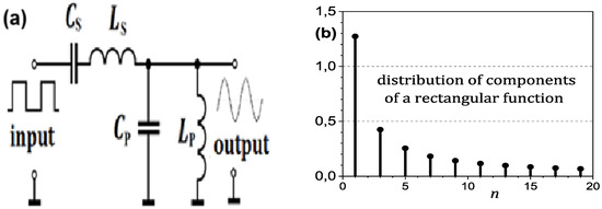
Figure 1.
Scheme of the band-pass filter (a) and the theoretical values of the amplitudes of subsequent harmonics contained in a square wave (b).
It consists of electric coils and capacitors with a high quality factor, with the serial branch consisting of a CS capacitor and an LS coil, while the other branch contains parallel-connected CP and LP elements. If we select these elements so that they meet the condition CSLS = CPLP, it turns out that at the resonant frequency f0, the series branch of CSLS will show zero reactance, while the parallel branch of CPLP will have a very high reactance at this frequency. Such diversification of the reactance of both branches will occur only for the selected frequency. All other harmonics will be largely eliminated and will practically not occur at the output of the filter. A rectangular signal contains many higher harmonic components whose amplitude is determined from the Fourier distribution [18]:
Figure 1b shows the theoretical values of the amplitudes of subsequent harmonics contained in a square wave.
The U1(t) waveform is a rectangular wave signal containing all harmonic (sine) components with higher frequencies, and the U2(t) waveform is a sine wave with the fundamental frequency f0 extracted from the rectangular wave signal. According to Kirchhof’s second law, it can be written that U1(t) − U2(t) = U12(t), which means that the difference in these voltages includes the sum of all higher harmonics except for the fundamental frequency f0,the output, and the signal of their difference.
In turn, Figure 2 shows the real waveforms of the rectangular signal U1(t) and the filtered signal U2(t). A slight deviation from the ideal square wave has no negative effect on the shape of the obtained sine wave at the filter output. In practice, as can be seen, the voltage shape on the LP magnetizing coil is correct, which proves the effectiveness of filtering by the band-pass system for both types of devices.
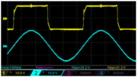
Figure 2.
Real waveforms of signals at the input and output of the band-pass filter at a frequency of f = 100 kHz. Time scale along the x-axis: 2 μs/div. Signal scale along the y-axis: 10 V/div. Signal amplitudes: yellow, 21.2 Vpp; aquamarine, 25.5 Vpp.
In order to produce an RMF, two or three separate pulsating fields must be superimposed, for example, by solenoid coils, which are excited by separate sine waveforms. Each component of the magnetic field must be placed in space at the correct angle, and the currents flowing in the magnetizing coils must flow with the correct phases. This operating principle is shown in Figure 3a,b below.
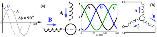
Figure 3.
The principle of creating a rotating magnetic field in a two-phase system (a) and in a three-phase system (b).
Circuits that follow this simple principle must supply sinusoidal currents to the magnetizing coils, for example, from high-power amplifiers. With 3-phase devices generating an RMF, three such amplifiers should be used, the cost of which, depending on the power and the frequency band, is high. A device fulfilling a similar task can be powered by rectangular signals if they are built on the basis of much cheaper switching modules. Their cost then does not exceed 10% of the price of systems with linear amplifiers.
2.1. Two-Phase RMF Generation System Powered by Rectangular Signals
Figure 4 shows a two-phase RMF generation system [16], in which a band-pass filter was used, powered by two rectangular signals shifted in phase by π/2 radians.
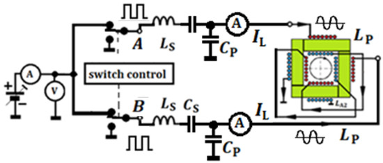
Figure 4.
Scheme of a two-phase system for generating a high-frequency rotating magnetic fieldpowered by rectangular signals. Parameters of the magnetizing coils: LP = 11.5 μH connected in parallel with capacitors: CP = 220 nF. Parameters of the coils: LS = 20 μH connected in series with capacitors: CS = 126 nF.
The LP magnetizing coils are wound on ferrite bars. In each phase there are two coils wound in opposition and connected in parallel with the Cp capacitors. In this case, the magnetic fluxes of each phase add up inside the ferrite circuit, as shown in Figure 5a,b for the respective times. In the case when through the coil of circuit A the magnetizing current IA reaches its maximum, then in circuit B the magnetizing current IB = 0. The situation changes after time T/4, when IA = 0 and IB = Imax.
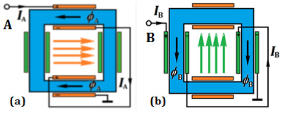
Figure 5.
RMF generation in a two-phase system with two pairs of Gramme coils. Currents and magnetic fluxes are shown for successive phases of sinusoidal waveforms (90°). In (a), the maximum current IA flows through circuit A while the current IB =0. In turn, in (b), after time T/4, IA = 0, while the current IB reaches its maximum flowing through circuit B.
When designing the device, the value of the amplitude of the magnetic field strength H in the middle part of the circuit can be initially estimated according to the expression [15,16]:
where IL is the amplitude of the magnetizing current (flowing through the LP coil), nis the number of turns on each ferrite bar, and lair is the length of the magnetic flux path in the air. The exact value of the magnetic field strength H is determined on the basis of the voltage induced in the probe coil inserted in the area of operation of the RMF, according to the formula:
where Sprobe = 0.00168 [m2] is the area of all windings for this probe coil, and f [Hz] is the frequency.
High-frequency current (IP) measurements can be made using a ferrite current transformer [14]. The material of this ferrite is 3C90, for which Bsat = 320 mT.
n-turns were wound on a ferrite core, to which a low-impedance resistor R2 was connected.
The primary winding consisted of a single wire carrying current I1, and a voltage U2 was induced in the secondary n-winding.
Current I1 can be calculated using the following equation, provided that R2 << XL:
where XL is the reactance of winding n.
The system shown in Figure 4 is powered from a regulated DC source, and the measurement of Udc and Idc allows us to additionally determine the electric power P supplied to the filter system loaded with a magnetic circuit. In turn, the high-frequency magnetizing currents IL were determined using current transformers [16] whose output voltage is linearly related to the value of the magnetizing current. It is worth adding that the capacitor CP together with the inductance LP, when tuned to the resonance frequency f0, shows a high impedance, and then the magnetizing current IL has an amplitude many times greater than the current flowing through the CSLS series branch.
In Figure 6, the phase and amplitude relationships between the rectangular-wave signals from the outputs of the switches A and B and the sinusoidal waveforms from the LP magnetizing coils from 1:7 windings are shown.
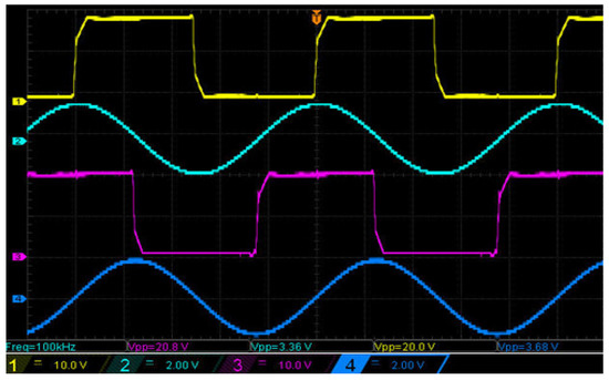
Figure 6.
Example waveforms of real rectangular and sinusoidal signals from the outputs of the switching system and on the LP magnetizing coils (from 1:7 coils) of the magnetic system. Time scale along the x-axis: 2 μs/div. Signal scales along the y-axis: yellow and purple, 10 V/div; aquamarine and blue, 2 V/div. Signal amplitudes: yellow, 20 Vpp; aquamarine, 3.36 Vpp; purple, 20.8 Vpp; blue, 3.68 Vpp.
2.2. Three-Phase RMF Generation System Powered by Rectangular Signals
The diagram of a three-phase RMF-generating device [17] shown in Figure 7 works according to a similar principle as previously presented. In both two- and three-phase systems, the bandpass filter parameters should meet the following criteria: LSCS ≅ LPCP.
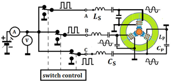
Figure 7.
Scheme of a three-phase RMF generation system with LSCS elements connected in series and LPCP elements connected in parallel, powered by rectangular signals with phases shifted by 120. Parameters of the magnetizing coils: LP = 6.3 μH connected in parallel with capacitors: CP = 401 nF. Parameters of the coils: LS = 20 μH connected in series with capacitors: CS = 126 nF.
The difference lies in the use of three switching modules and three band-pass filters and a slightly different design of the magnetic system. In this case, a ferrite torus was used, which reduces the magnetic reluctance Rm of the magnetic flux ϕ, which allows to achieve a greater value of the amplitude of the magnetic field strength H in the central part of the system.
Due to the use of a three-phase system, the arrangement of the three coils of the magnetizing circuits was set every 120 angular degrees, as shown in Figure 8.
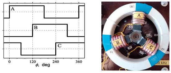
Figure 8.
Example waveforms of three rectangular signals A, B, and C (on the (left)) and appearance of the magnetic system with three magnetizing coils LP wound on ferrite rods (on the (right)).
Figure 9 shows three sine signals proportional to the voltages on the LP coils from 1:5 windings.
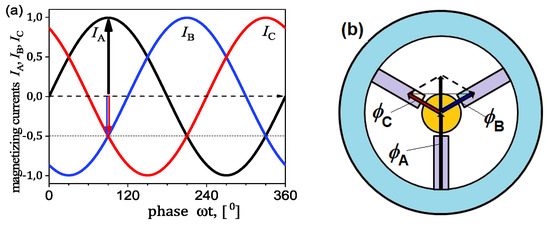
Figure 9.
Magnetizing currents flowing through each pair of coils IA, IB, and IC (a), the distribution of magnetic fluxes inside the torus at the moment when the phase angle ωt = 90 (b).
The instantaneous values of the magnetizing currents in individual pairs of coils are described by the following formula:
Figure 9a shows that for ωt = 90, the instantaneous value of the magnetizing current in circuit A is IA = 1, and the other currents have the values IB = −0.5 and IC = −0.5.
It can be assumed that a positive value of the magnetizing current means that the flux generated by such a current flows into the center of the torus, while a negative value of the magnetizing current causes the flux to flow from the central air region towards the torus.
Figure 9b shows the position in space of all the magnetic flux vectors ϕA, ϕB, and ϕC and their components projected to the direction of the vector whose value is the highest at a given moment. This means that the resultant magnetic flux created, for example, by the coils of circuit A and the remaining fluxes ϕB and ϕC, creates a resultant flux of a rotating magnetic field, the value of which is 50% greater than the flux ϕA.
Figure 10 shows the time waveforms of the voltages induced in single turns wound on each core in circuits A, B, and C. The phase shift between these signals is 120 and the period T = 1/f = 10 μs.
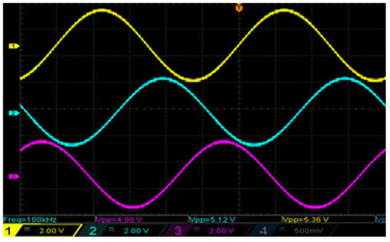
Figure 10.
Example waveforms of sinusoidal signals on the magnetizing coils from 1:5 coils LP. Time scale along the x-axis: 2 μs/div. Signal scales along the y-axis: yellow, aquamarine, and purple, 2 V/div. Signal amplitudes: yellow, 5.36 Vpp; aquamarine, 3.36, 5.12 Vpp; and purple, 4.96 Vpp.
3. Comparison of Electrical Properties of Both Systems Generating an RMF
Both RMF-generating systems were tested to determine their basic technical parameters.
The amplitudes of the magnetic field strength H and the necessary voltage Udc from the DC source needed to generate this strength were compared. In addition, the values of the magnetizing currents IL flowing through the LP coils were determined.
The relationships H(Udc) shown in Figure 11 show a high linearity, and the three-phase system allows us to obtain more than twice (2.22) the value of the amplitude H compared to the two-phase system at the same voltage Udc.
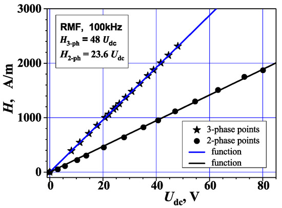
Figure 11.
The dependence of the RMF intensity amplitude H on the voltage Udc for a two- and three-phase system. Measurement accuracy: 5%.
A similar linearity was obtained between the magnetizing currents IL and the supply voltage Udc (Figure 12). In this case, a current transformer was used to measure the magnetizing current, where the value of the primary winding current (IL) was recalculated on the basis of the secondary voltage across the resistor (practically shorting the transformer). In this case, for a specific supply voltage Udc in a three-phase system, the current was 92% higher than in a two-phase system.
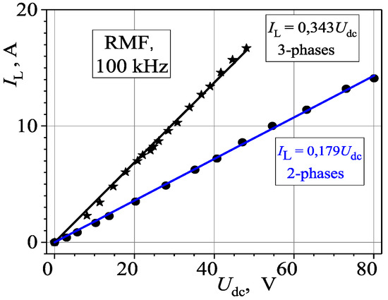
Figure 12.
Dependence of the amplitude of the magnetizing current IL on the voltage Udc for a two- and three-phase system. Measurement accuracy: 5%.
The two-phase magnetic system uses 3C90 ferrite shapes with a cross section of 25/12 mm (SFe = 0.0003 m2). In this device, the air gap lair = 35 mm, which at a magnetizing current of 25 A allows for an air gap of Hair = 10 kA/m. (https://doi.org/10.1016/j.jmmm.2022.170198, accessed on 18 November 2022). Taking into account the air gap area (Sair = 35*25 mm2), we obtain a value of Bair ≈12.6 mT.
It is clear that this is only 4.2% of the saturation induction for ferrite. Therefore, saturation (BSAT ≈ 320 mT) was probably not the main cause of the nonlinearity of the magnetic system.
On the other hand, in the three-phase system, the air gap was almost twice as small, and the nonlinearity effect occurred more easily in this case. This matter really requires clarification as to whether the cause was the presence of higher harmonics or nonlinearity resulting from magnetic saturation of the material.
The electrical power P supplied to both RMF generation systems was also compared as a function of the magnetic field strength H. As shown in Figure 13, the two-phase system consumes less electrical power than the three-phase system. However, it can be seen that this relationship is not linear in both systems, likely due to the nonlinear effects of the ferrite materials. It is worth noting that in the three-phase system, the magnetizing coil LP had only n = 5 turns, while in the two-phase system, n = 7. This can also explain the differences in the nonlinearity of the two systems. Figure 14 shows, for example, the calorimetric effect with the APG513 magnetic fluid under the influence of the RMF for a few selected frequencies. As can be seen, to achieve dT/dt > 100 mT/s, H = 5 kA/m at f = 150 kHz should be used. This estimated value of f·H =7.5·10−8 [As/m] is slightly higher than the recommended value in the Brezovich criterion: 4.8·10−8 [As/m]. The RMF parameters obtained in Figure 14 allow the use of a similar design solution in magnetic hyperthermia treatments.
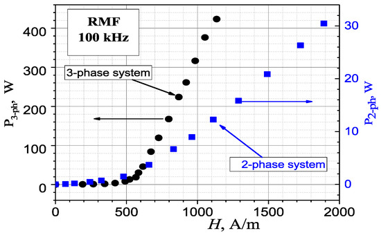
Figure 13.
Dependence of the power P drawn from the DC source on the magnetic field strengthamplitude H for a two- and three-phase system. Measurement accuracy: 5%.
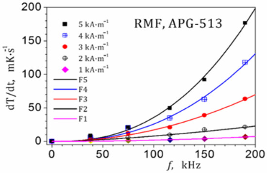
Figure 14.
Dependencies of the rate of temperature increase dT/dt as a function of RMF frequency for H =1 kA/m, 2 kA/m, 3 kA/m, 4 kA/m, and 5 kA/m, obtained from measurements in a two-phase system. Measurement accuracy: 5%.
The parameters of magnetic circuits with a two-phase system are shown in Table 1, while Table 2 shows similar data for three-phase systems. As can be seen from the comparison of both systems, the coupling factor k has a very small value. Namely, k = 0.0165 for a two-phase system and k = 0.00222 for a three-phase system.

Table 1.
Parameters of magnetic circuits with a two-phase system.
Table 2.
Parameters of magnetic circuits with a three-phase system.
4. Conclusions
- At a fixed value of the supply voltage Udc, the values of the magnetizing current IL and the amplitude H of the rotating magnetic field strength are about twice as large for a three-phase system as for a two-phase system.
- A comparison of the electrical power consumed by both RMF generation systems shows that the three-phase system draws more power to generate the same magnetic field strength amplitude.
- This effect can be explained by the nonlinearity of the magnetic materials, as well as the different number of turns in the magnetizing coils and different shapes of external ferrite (torus or square).
- RMF generation using square-wave voltages to power the magnetic systems is much cheaper than powering them with sinusoidal signals from expensive high-power, high-frequency amplifiers.
Funding
The studies were supported financially in part by statutory fund of the Faculty of Physics and Astronomy, Adam Mickiewicz University (506000/606/4203000000/BN002025).
Data Availability Statement
The original contributions presented in the study are included in the article, further inquiries can be directed to the corresponding author.
Conflicts of Interest
The author declare no conflicts of interest.
References
- Rosensweig, R.E. Heating magnetic fluid with alternating magnetic field. J. Magn. Magn. Mater. 2002, 252, 370–374. [Google Scholar] [CrossRef]
- Maniotis, N.; Maragakisb, M.; Vordosb, N. A comprehensive analysis of nanomagnetism models for the evaluation of particle energy inmagnetic hyperthermia. Nanoscale Adv. 2025, 7, 4252. [Google Scholar] [CrossRef] [PubMed]
- Carrey, J.; Mehdaoui, B.; Respaud, M. Simple models for dynamic hysteresis loop calculations of magnetic single-domain nanoparticles: Application to magnetic hyperthermia optimization. J. Appl. Phys. 2011, 109, 083921. [Google Scholar] [CrossRef]
- Raikher, Y.L.; Stepanov, V.I. Power losses in a suspension of magnetic dipoles under a rotating field. Phys. Rev. E 2011, 83, 021401. [Google Scholar] [CrossRef] [PubMed]
- Dutz, S.; Hergt, R. Magnetic particle hyperthermia—A promising tumortherapy? Nanotechnology 2014, 25, 452001. [Google Scholar] [CrossRef] [PubMed]
- Makridis, A.; Kazeli, K.; Kyriazopoulos, P.; Maniotis, N.; Samaras, T.; Angelakeris, M. An accurate standardization protocol for heating efficiency determination of 3D printed magnetic bone scaffolds. J. Phys. D Appl. Phys. 2022, 55, 435002. [Google Scholar] [CrossRef]
- Pankhurst, Q.A.; Connolly, J.; Jones, S.J.; Dobson, J. Applications of magnetic nanoparticles in biomedicine. J. Phys. D Appl. Phys. 2003, 36, 167–181. [Google Scholar] [CrossRef]
- Abu-Bakr, A.; Zubarev, A. Hyperthermia in a system of interacting ferromagnetic particles under rotating magnetic field. J. Magn. Magn. Mater. 2019, 477, 404–407. [Google Scholar] [CrossRef]
- Hiergeist, R.; Andra, W.; Buske, N.; Hergt, R.; Hilger, I.; Richter, U.; Kaiser, W. Application of magnetite ferrofluids for hyperthermia. J. Magn. Magn. Mater. 1999, 201, 420–422. [Google Scholar] [CrossRef]
- Brezovich, I.A. Low Frequency Hyperthermia: Capacitive and Ferromagnetic Thermoseed Methods. Medical Phys. Monogr. 1988, 16, 82–110. [Google Scholar]
- BenZvi, I.; Chang, X.; Litvinienko, V.; Meng, W.; Pikin, A.; Skaritka, J. Generation high-frequency fields with low harmonic content. Phys. Rev. Accel. Beams. 2011, 14, 092001. [Google Scholar] [CrossRef]
- Bekovi’c, M.; Trlep, M.; Jesenik, M.; Hamler, A. A comparison of the heating effect of magnetic fluid between the alternating and rotating magnetic field. J. Magn. Magn. Mater. 2014, 355, 12–17. [Google Scholar] [CrossRef]
- Beković, M.; Trbusic, M.; Trlep, M.; Jesenik, M.; Hamler, A. Magnetic fluids’ heating power exposed to a high-frequency rotating magnetic field. Adv. Mater. Sci. Eng. 2018, 2018, 6143607. [Google Scholar] [CrossRef]
- Wojciechowski, R.M.; Skumiel, A.; Kurzawa, M.; Demenko, A. Design, application and investigation of the system for generation of fast changing, rotating magnetic field causing hyperthermic effect in magnetic liquids. Measurement 2022, 194, 111020. [Google Scholar] [CrossRef]
- Skumiel, A.; Wojciechowski, R.M. Two-Phase System for Generating a Higher-Frequency Rotating Magnetic Field Excited Causing Hyperthermic Effect in Magnetic Fluids. Energies 2022, 15, 8326. [Google Scholar] [CrossRef]
- Skumiel, A.; Musiał, J. The use of Gramme coils in a 2-phase system for generation of a high frequency rotating magnetic field. J. Magn. Magn. Mater. 2022, 564, 170198. [Google Scholar] [CrossRef]
- Skumiel, A. Comparison of winding configurations of a 3-phase system for generating a rotating magnetic field powered by rectangular signals. J. Magn. Magn. Mater. 2023, 579, 170851. [Google Scholar] [CrossRef]
- William, A.B.; Leonard, L.G. Introductory Network Theory; PWS Engineering: Boston, MA, USA, 1985. [Google Scholar]
Disclaimer/Publisher’s Note: The statements, opinions and data contained in all publications are solely those of the individual author(s) and contributor(s) and not of MDPI and/or the editor(s). MDPI and/or the editor(s) disclaim responsibility for any injury to people or property resulting from any ideas, methods, instructions or products referred to in the content. |
© 2025 by the author. Licensee MDPI, Basel, Switzerland. This article is an open access article distributed under the terms and conditions of the Creative Commons Attribution (CC BY) license (https://creativecommons.org/licenses/by/4.0/).