1. Introduction
Giant inverse magnetocaloric materials have gained recent attention in the scientific community due to their high magnetic-to-thermal energy conversion efficiencies and potential for eliminating environmentally harmful chemicals typically used in conventional vapor-compression refrigeration units. Residential and commercial heating and cooling appliances account for nearly 40% of the United States’ energy consumption, totaling 20.26 quadrillion British thermal units (BTU) annually. As global populations continue to grow, the amount of energy allocated for heating and cooling applications is expected to increase by 84% by the year 2050, compared to energy levels from 2010 [
1,
2]. The environmentally damaging fluids used in vapor compression systems, such as chlorofluorocarbons (CFCs) or hydrofluorocarbons (HCFCs) [
3,
4], are well-known to be leading contributors to greenhouse gas emissions and can destroy stratospheric ozone [
5,
6].
Solid-state refrigeration devices, such as magnetocaloric and thermoelastic regenerators, have the potential to mitigate greenhouse gas emissions [
7], as they do not require HCFCs in thermodynamic cooling cycles. In a report submitted to the U.S. Department of Energy [
8], magnetocaloric and thermoelastic technologies are projected to reduce energy demands for HVAC systems in both commercial and residential sectors by at least 20%. However, to succeed in that goal, there must be further development of caloric materials. Thus, the authors aim to define an analytical approach for computing a performance metric useful for comparing the energy conversion efficiency in novel solid-state refrigerant materials to facilitate high-throughput performance screening.
In previous works, Wood and Potter developed a thermodynamic metric, namely the refrigeration capacity (
RC), that could be applied to materials that exhibited second-order magnetic transitions without hysteretic loss [
9]. Nearly 20 years following their work, Pecharsky and Gsneidner conceived a similar metric, namely the relative cooling power, RCP, which was applied to the first-order magnetostructural transition observed in GdSiGe [
10,
11]. They also employed the RCP to compare materials that exhibited a second-order magnetic transition, such as pure Gd [
10]. However, using the RCP to compare materials that exhibited hysteretic losses across magnetostructural transitions with those that did not (e.g., across purely magnetic second-order transitions) led to misleading comparisons. More recently, other metrics applicable to materials exhibiting first-order magnetostructural transitions have been derived by the present author [
12], Moya [
13,
14], and Brück [
15]. For instance, Brück et al. defined a coefficient of performance, COP, which accounted for hysteretic losses through its implementation and was applicable to the physics across first-order structural phase transformations. It was mentioned that, in quantifying the applied magnetic-work required to generate the cooling in the magnetocaloric material (i.e., energy input), the isothermal magnetization loops needed to be numerically integrated. Data for complete magnetization loops across magnetostructural transitions were limited in the literature and were cumbersome to digitize.
Here, we aim to analytically compute the metric so that commonly measured and reported materials properties can be used to quickly compare the performance of novel magnetocaloric materials. In this way, solid refrigerants that exhibit a first-order magnetostructural transition with transformation hysteresis can be quickly assessed. First, the thermodynamics governing the conventional (second-order) caloric effects in solids are briefly described, which can be defined for any externally applied stimuli (thermodynamic force) that influences a material’s free energy. The thermodynamics are then incorporated into Wood and Potter’s
RC parameter. Next, the thermodynamics governing first-order structural phase transformations are described. The entropy change and adiabatic temperature change are derived from the Clausius–Clapeyron relationship and a method developed by Porcari et al., [
16,
17], respectively. These are later applied to Wood and Potter’s
RC parameter, and the disadvantages of employing this metric to first-order structural transitions are revealed.
Finally, we present an analytical approach to compute the coefficient of refrigeration performance (CRP) that is directly applicable to first-order structural phase transitions. The analytical approach accounts for hysteretic losses and employs basic and commonly reported materials properties in the literature, rather than cumbersome digitized magnetization data. The development of the analytical CRP is followed with a discussion and examples used for comparing the caloric effects in first-order magnetostructural materials.
2. Thermodynamic Quantities of Interest
A caloric, or thermal, effect is defined by a material’s isothermal entropy () or adiabatic temperature () change in response to some external stimulus (force). For the elastocaloric effect (ECE), this stimulus is mechanical load, and for the magnetocaloric effect (MCE), a magnetic field. Reversible heating and cooling effects can be generated in a solid material by a change in the material’s free energy, which might include latent heat effects from a structural transition. Heating can also be generated through any irreversible processes that occur at the time of applying the external field. Magnetic and structural hystereses serve as indicators that thermodynamically irreversible processes take place, and through the second law of thermodynamics, the entropy produced (and thus heat) from these irreversible processes will always be greater than zero.
The internal energy of a substance changes with an applied thermodynamic “force”, such as stress, temperature, and magnetic field. These forces do not depend on the material’s volume and are referred to, herein, as intensive thermodynamic variables.[
18] Since we aim to determine the caloric effects resulting from a change in internal energy, we consider the Gibbs free energy,
, which implicitly assumes intensive variables are applied to the substance in question during experiments [
18]. Here, the
describes the free energy of a single structural phase. The change in free energy,
, of that phase is defined as [
18]
where
is specific volume (m
3·kg
−1),
is hydrostatic pressure (Pa),
is the entropy (J·kg
−1·K
−1),
is temperature (K),
are extensive (volume dependent) material properties, such as bulk magnetization
(emu·g
−1) or specific strain
(m
3·kg
−1), and
are their thermodynamic intensive-force conjugates, such as applied magnetic field,
(Tesla), or uniaxial stress,
(Pa), respectively. Note that
is the permeability of free space in Henry·m
−1, and
is the applied magnetic field in A·m
−1.
The isothermal entropy change defining the caloric effect can then be quantified using Equation (1). This is performed by employing Maxwell relations, first assuming that the application of the external stimuli is performed at atmospheric pressure and that all other applied forces are constant, i.e.,
. The entropy,
, is expressed as
The forces that are assumed constant in Equation (2) are denoted by subscripts. Similarly, other extensive thermodynamic quantities can be solved for from Equation (1) using the same approach. In the case, below, pressure and temperature are assumed constant. Here,
can be expressed as
where
,
, and all other
are constant intensive variables.
Next, Equations (2) and (3) can be differentiated with respect to the other’s independent variable. Equation (2) is differentiated with respect to
resulting in
and Equation (3) with respect to
, resulting in
Assuming that the second partial derivative of
is smooth and continuous, the right-hand side of Equations (4) and (5) are identical, and therefore, the left-hand sides are also mathematically equivalent. The incremental isothermal entropy change and “caloric effect”,
, from stimulus
can then be denoted as
which simplifies to
In Equation (7), the isothermal entropy change has been derived for any single phase exposed to the intensive force
in
. It is important to note that, in experiments where strain drives the caloric effect and is thus the independent variable, the Helmholtz free energy expression should be employed, instead of
, to insure consistency between the measured and predicted caloric behaviors [
19].
2.1. Conventional Magnetocaloric Cooling with Second-Order Transitions
A wide range of crystalline and amorphous materials exhibit the MCE. Laves phases [
20], ferromagnetic lanthanum manganites [
21,
22,
23], and other rare-earth containing crystalline compounds [
24,
25,
26,
27] are commonly studied. Many Laves phase compounds, such as HoCo2 [
28,
29], TbCo2 [
30], and TbFe2 [
31], are of interest, because they exhibit a significant change in magnetization,
, across their ferromagnetic/paramagnetic Curie temperatures,
. Many well-performing conventional MCE materials are not employed in regenerative cycles due to limited availability and the cost of rare earths.
If a magnetic field,
, is applied to a magnetocaloric refrigerant, the resulting entropy change is defined as
by Equation (7), where
has been replaced with
and is the energetic conjugate of
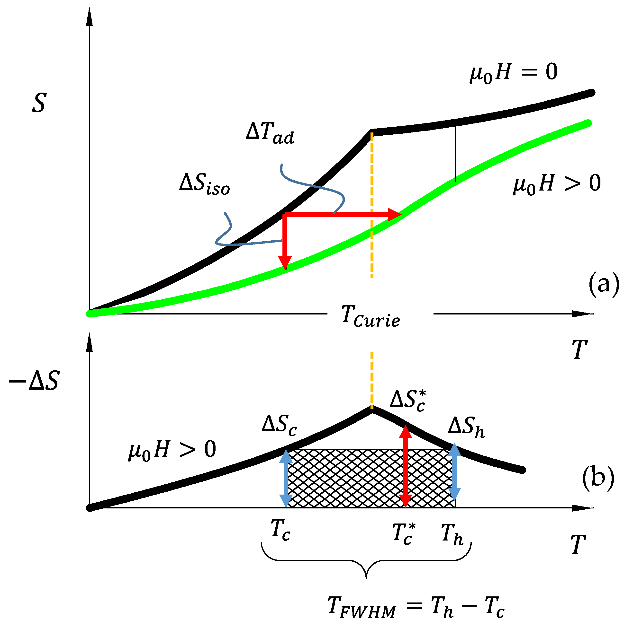
. The MCE, or magnetic field-induced isothermal entropy change across a second-order magnetic transition, is illustrated in
Figure 1a,b.
In
Figure 1a, the entropy versus temperature diagram of a ferromagnetic material is depicted around its
. Under zero magnetic field (top curve), the entropy is shown to exhibit a cusp at
[
32]. According to Equation (2), the entropy curve is defined by the partial derivative of the
with respect to temperature. Clearly, the second temperature derivative of the free energy, i.e.,
, exhibits a discontinuity at
, thus making the change in magnetization at
a second-order magnetic transition. Interestingly, the assumption of commutativity, described above, no longer holds exactly at
due to the inability to quantify the derivative of
. However, at temperatures above and below
, Equation (7) is applicable for determining magnetic field-induced
.
Upon applying
to a ferromagnetic material around its
, the total entropy (magnetic disorder) decreases, as depicted in
Figure 1a,b. This can manifest an increase in temperature. Consequently, the MCE in most ferromagnetic materials that exhibit second-order magnetic transitions is achieved through adiabatic or isentropic demagnetization, i.e., removing the applied magnetic field.
The adiabatic temperature change corresponding to a decrease in entropy is illustrated by a red horizontal arrow labeled as
in
Figure 1a. The magnitude of
in a single structural phase material (described with the above Gibbs free energy) can be derived using the following thermodynamic assumptions and analyses. It is assumed that the total change in entropy,
, is a function of all other thermodynamic quantities as posited by the Truesdell’s theory of equipresence and the structure of thermodynamic state functions [
33]. As such,
is defined as
According to
Figure 1a, the
is produced when
. Assuming isobaric (
) and isentropic (
) conditions in Equation (8) to match the condition of adiabatic experiments, Equation (8) reduces to
when only one driving force,
is applied. Substituting the Maxwell relation from Equation (6) into (9) for
results in
where by the entropy change generated from applying
can be moved to the left side of the equality. Thus,
where
per the second law of thermodynamics, and
is the isobaric heat capacity [
18]. Therefore,
Finally, the terms in Equation (12) can be separated and integrated, leading to
where the adiabatic temperature change can be computed for any isochoric driving force,
, if the isobaric heat capacity,
, and extensive
histories are known. Oftentimes,
is assumed to be independent of the driving force,
, and
is approximated as [
34]
It is important to note that Equation (14) has been developed using for a single structural phase. Furthermore, this is simply an approximation, assuming only small fluctuations occur in by applying the external stimuli. Moreover, in Equation (14) is nominally assumed to equal the starting temperature at which is applied during the adiabatic temperature change.
2.2. Wood and Potters Refrigeration Capacity for Magnetic Cooling
The refrigeration capacity (
RC) defines the suitability of a magnetic material for cooling applications and was originally conceived by Wood and Potter [
9] approximately forty years following the seminal work of Weiss and Piccard [
35]. Wood and Potter proposed that a measure of how well a magnetic refrigerant will operate should be based on its capability to perform thermal work through field cycling used in magnetic regenerative heat cycles. They considered that the entropy change at the cold end of a heat cycle should not exceed that at the hot end to satisfy the second law of thermodynamics. As such, the “thermal work” that was performed by a magnetocaloric material was defined as the entropy change achieved at the cold temperature reservoir of a heat cycle,
, multiplied by the temperature gradient across which the heat was moved,
. Originally, the
was defined as the difference between the hot (
) and cold (
) reservoir temperature of a regenerative cycle, i.e.,
. Due to the ambiguity of the proposed hot and cold temperature reservoirs, in practice, these temperatures were assumed to be the full-width-half-maximum (
) of the entropy change versus temperature diagram, as shown in
Figure 1b [
32].
Figure 1b illustrates the
RC computed for conventional second-order magnetocaloric refrigerants from the above entropy change versus temperature diagram. To generate the entropy change versus temperature curves, the difference was computed between the zero field (
) and applied field (
) curves from
Figure 1a. As shown in
Figure 1b, an entropy change at some cold temperature,
, is defined as
, whereas an entropy change of
is achievable at temperature
. Thus, the
RC, was defined as [
9]
Clearly, the goal of much present-day research is increasing the
RC in state-of-the-art MCE materials [
7,
36], because it corresponds to the amount of reversible thermal work performed by the refrigerant.
In magnetocaloric refrigerants exhibiting a second-order magnetic transition, the largest entropy change occurs around the
, but this temperature does not change as a function of applied field. As such, applying greater magnetic fields to second-order magnetocaloric compounds simply increases the
and only marginally broadens the entropy change peak (i.e.,
in Equation (15)). To compare materials using Wood and Potter’s
RC parameter, Equations (14) and (7) were substituted into Equation (15), so
. Using
in place of
leading to a thermodynamic performance metric for second-order phase transforming materials in heat cycles around their
[
10]. It is important to note, however, that
and
are both dependent on the applied field level and operating temperature. In the following section, we describe the magnetocaloric effects that are generated across
first-order magnetostructural phase transitions and how they differ from those in the above sections. Performance criteria are analytically developed for reversible behavior in first-order materials so they may be properly compared with reversible second-order systems.
3. Thermodynamics of Giant Caloric Effects across First-Order Meta-Magnetic Transitions
First-order magnetostructural transitions are observed in many multifunctional alloys [
37]. For simplicity, we focus on the observed behaviors in a well-known NiMnIn meta-magnetic shape memory alloy (MMSMA) [
38,
39]. MMSMAs are rare-earth-free intermetallic compounds that exhibit a reversible first-order magnetostructural diffusionless phase transformation between low temperature martensite (M) and high temperature austenite (A) and are candidates for cooling applications [
40,
41,
42]. In our analyses, isothermal magnetization data measured in Ni
48Mn
38In
14 (at.%) polycrystals were used to describe the meta-magnetic behavior across first-order magnetostructural transitions and the caloric effect. The NiMnIn polycrystals, herein, were subjected to a homogenization treatment at 1123 K for 24 h in a protective argon atmosphere and then water quenched.
At temperatures below a critical transformation temperature,
, NiMnIn alloys are composed of a non-magnetic M-phase (paramagnetic, superparamagnetic, etc.) [
43,
44,
45,
46,
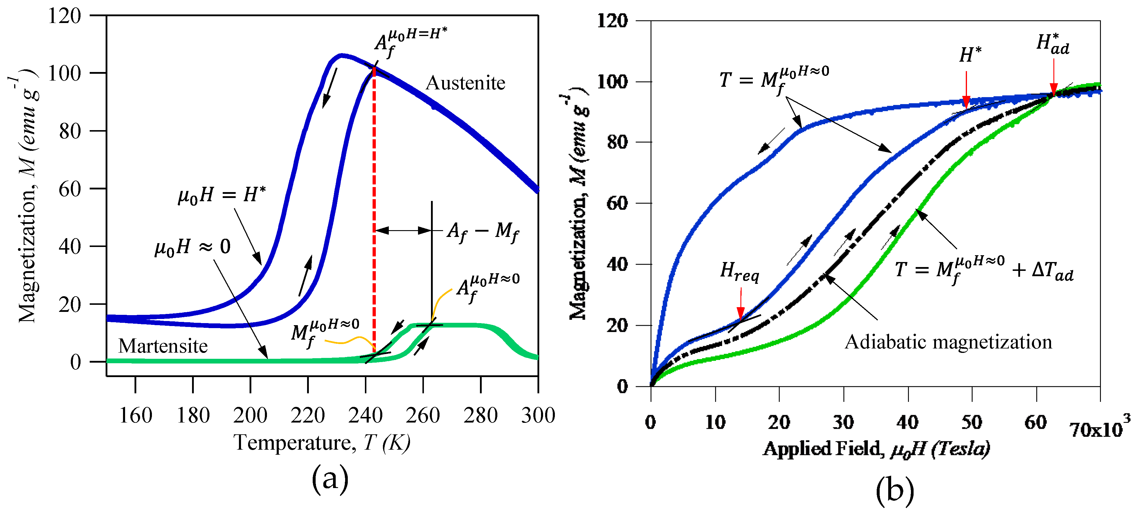
47]. This is illustrated by the thermomagnetic curves in
Figure 2a. On heating the M-phase in a small
, the MMSMA begins to spontaneously magnetize (see green curve) as it transforms into the high temperature A-phase and is accompanied by an endothermic (cooling) reaction from the latent heat of the martensitic transition. On heating, critical M-to-A transformation temperatures are referred to as the austenite start (
temperature and austenite finish (
) temperatures. Conversely, cooling causes an exothermic A-to-M transformation at the critical temperatures denoted as martensite start (
) and martensite finish (
). The difference in
and
has been used to describe energy barriers to the martensitic transformation, including elastic and irreversible parts [
48,
49,
50,
51,
52], and is the main reason for developing an analytical performance metric for only the reversible behavior in first-order materials, as second-order materials do not exhibit these same energy losses or barriers. Moreover, second-order materials exhibit the conventional magnetocaloric effect as described by Equation (7), but first-order materials exhibit magneto-structural transformations which are accompanied by a latent heat component and therefore exhibit “giant” magnetocaloric effects.
Upon applying a constant magnetic field,
, to the MMSMA and measuring magnetization across the reversible martensitic transition, the
,
,
, and
temperatures experience a decrease (see blue curve in
Figure 2a), indicating that the magnetic field stabilized the high-temperature ferromagnetic A-phase. Indeed, each critical temperature exhibits a unique sensitivity to the applied field, also referred to as the Clausius–Clapeyron (CC) slopes,
,
,
, and
. Often, in the literature, these slopes are assumed to be equivalent to
; however, this can be an oversimplification. In inverse giant MCE materials, the CC slopes are negative in sign.
If the MMSMA is held at constant temperature
under zero magnetic field,
, then there exists a field level (
) at which the M-phase will completely transform to the A-phase, as shown in
Figure 2a by a vertical red dashed line. The magnetization response during this isothermal magnetic field-driven transformation at
is depicted in
Figure 2b by a blue curve. To complete the isothermal transformation at
, the
must effectively decrease (at the rate defined by
) to match
. Therefore, we can define
as the field level needed achieve a complete and reversible isothermal martensitic transformation at
, as
[
52]. In this expression,
is assumed to be a positive quantity that simply denotes the sensitivity of the
temperature to the applied
. Similarly, the magnetic field required to initiate the meta-magnetic transition at
can be defined by
, assuming
is a positive quantity. In this context of isothermal meta-magnetic magnetic field-driven transformations, the volume fraction of stabilized A-phase,
, can be computed as
, where
.
Clearly, if the MMSMA is constrained to a constant temperature equal to and then is applied, the complete M-to-A transition will occur. Moreover, subsequent removal of the field will produce the complete A-to-M transformation, making it cyclically reversible. If the same process was performed above , only partial or no transformation will occur on subsequent field cycling.
The magnetization and demagnetization response across the complete magnetic field induced transformation at
in NiMnIn is depicted (blue) in
Figure 2b up to
. In application, the endothermic reaction resulting from the M-to-A transition during adiabatic loading contributes to the temperature change of the MMSMA. Therefore, if the MMSMA was originally exposed to a magnetic field large enough to initiate transformation (see
in the figure) at
, the adiabatic temperature change must be overcome by applying an even greater magnetic field to progress the transformation to completion. For instance, if the complete M-to-A transformation produced
of −5 K, then the temperature barrier that must be overcome to complete the transition could be described by
. In terms of quantifying the magnetic field needed to complete the adiabatic transition, we assume the starting temperature is less than
by an amount equal to
. The magnetic field required to complete the adiabatic transformation at
, shown in
Figure 2b as
, was defined as
, and is again a positive quantity by assuming
is positive. To illustrate the adiabatic magnetization curve up to
, we have depicted an isothermal magnetization curve of our NiMnIn alloy at a temperature lower than
(green) and then found the average magnetization response (see dash-dot-dot curve) between the two temperatures. The adiabatic magnetization curve is essential for later development of the analytical CRP, as it defines the input energy required by the MMSMA to achieve the giant MCE.
First-order phase transitions are associated with a change in crystal symmetry (structure), which implies the
is discontinuous at the thermodynamic equilibrium temperature,
. The free energy above and below
describe that of two separate structural phases with independent physical properties including
,
,
, etc. At
, thermodynamic equilibrium between the two phases leads to the well-known CC relations [
18,
52,
53]. According to Equation (1), the
in either phase of the bulk material is influenced by external stimuli including hydrostatic pressure, temperature, and
(stress or magnetic field).
In the case of M-to-A first-order structural phase transitions [
49,
53,
54,
55] the
of each phase is equivalent at the point of the transition; thus, so is their differential,
Since each phase is exposed to the same driving forces at the point of transition,
Assuming the phase transition occurs in a constant pressure atmosphere,
, Equation (17) can be simplified to
Or
where
is the entropy change, or difference, between the two phases at
,
is the measured change in the
ith extensive property across the first-order transition, and
is the inverse CC slope [
53]. For partial transformations, i.e.,
, only a fraction of the
and
are achieved.
Equation (19) is applicable to magnetocaloric materials that exhibit first-order magneto-structural phase transitions, such as NiMnIn, where
and
= ; thus,
and
for a complete transformation. Equation (19) appears to be similar to Equation (7); however, these two expressions were derived under dissimilar thermodynamic conditions and therefore provide the
for fundamentally different processes. There has been much debate in the literature whether Equation (7) and its discretized form [
56] are applicable to quantify
across first-order transitions [
57]. While we recognize the large body of contributing discussions, this topic is out of the scope of the present work.
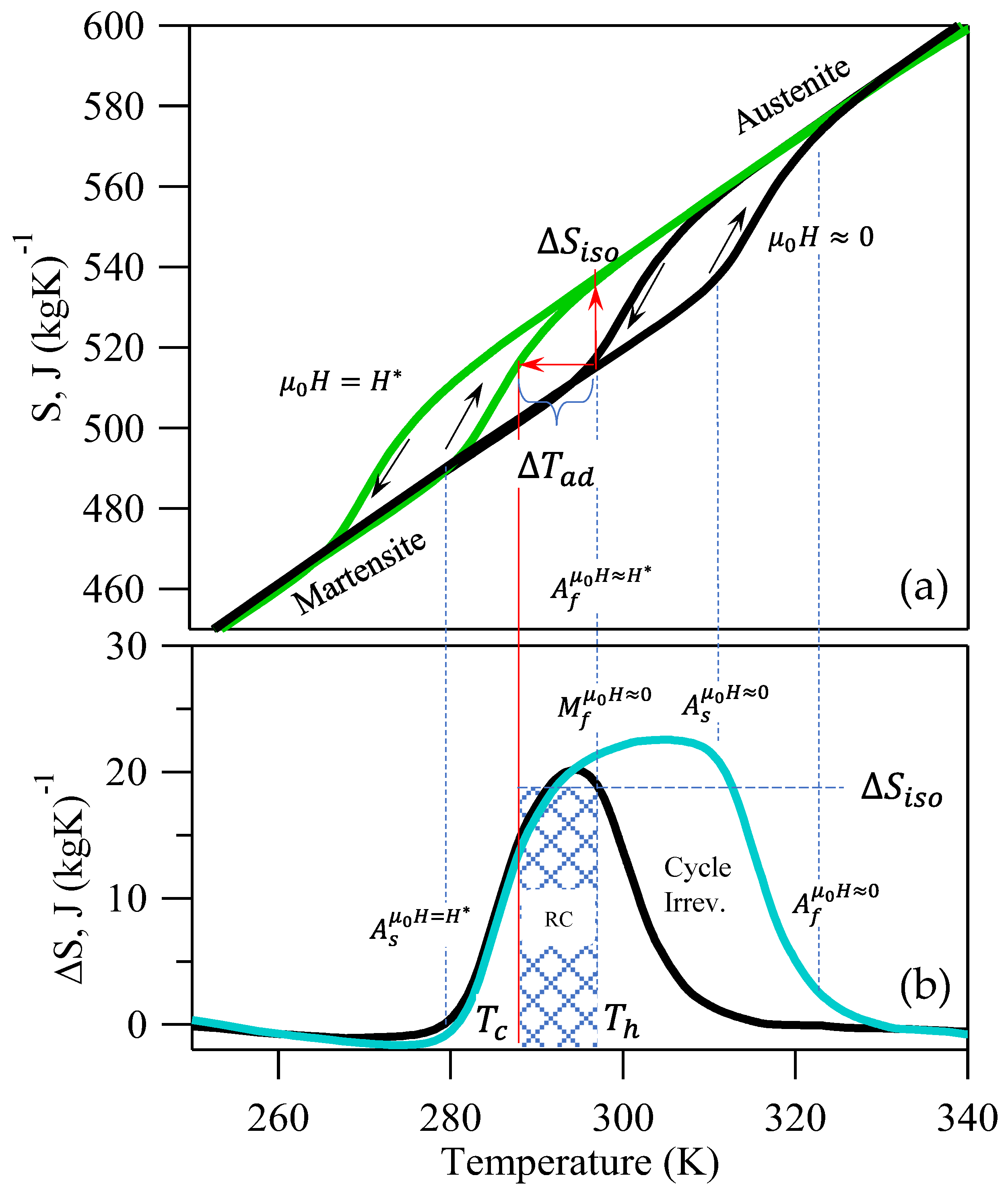
Using the described physics, we aim to develop an analytical form for the CRP that accounts for the cyclic irreversibility in first-order materials. We thus turn our attention to the entropy (
) versus temperature (
) diagrams, as was done with second-order materials (in
Figure 1). The isofield total
vs.
curves are depicted in
Figure 3 for our NiMnIn alloy [
52]. Since
is an extensive thermodynamic property, its behavior parallels the thermomagnetic response depicted in
Figure 2a. On heating the M-phase under no applied magnetic field, the MMSMA undergoes a structural transition starting at the
temperature and finishing at
, as indicated by the abrupt increase in
. On subsequent cooling, a thermal hysteresis is clearly observed when the material transforms back to the M-phase, and the
decreases abruptly.
Similar to the thermomagnetic response in
Figure 2a, the
vs.
response in
Figure 3a depicts a decrease in transformation temperatures under
. It can be seen clearly in
Figure 3a that if the MMSMA was originally at the
temperature and
was applied, then
will equal approximately the entropy difference between A and M. Applying this field results in a decrease in critical transformation temperatures.
Using the applied- and zero-field entropy versus temperature (
) data in
Figure 3, the entropy change,
, has been plotted below by computing the difference between the curves. The entropy change versus temperature depicted by the
curve in
Figure 3 and the corresponding labels are representative of the physics in all inverse NiMn-based first-order magnetostructural transitions. The cyan curve describing the entropy change represents those which are most commonly reported in giant magnetocaloric studies of MMSMAs [
12]. It is crucial to note that the features of the
curve align with critical transformation temperatures from the
diagram above, so they have been labeled explicitly.
Typically, in studies on giant MCE materials, the RC is computed using the commonly reported cyan curve by multiplying by , as was done in Equation (15). Note the encompasses the thermal hysteresis of the diagram above. If field cycling was performed at a temperature above , the MMSMA would only exhibit a partial entropy change on the first field ramping and zero on subsequent, and therefore would be cyclically irreversible—a large difference in the behavior that was described for second-order materials.
As mentioned in
Section 2.2,
, where
was assumed to equal
, and more recently,
[
10,
15]. In first-order materials, we propose
, which is nearly equivalent to the entropy change across the transition (see Equation (19)). It is interesting to note that
appears to be related to critical transformation temperatures in
Figure 3. Since
, we assume
, or
and
. Note that if
, the
RC parameter will yield erroneously high values. Since it is assumed that
,
will be reversible with field cycling. Moreover,
is expected to be cyclically reversible under these constraints.
Oftentimes, in the literature,
is approximated using Equations (8)–(14) [
58] for first-order phase transitions. However, through the author’s experience, this method of computing
often leads to approximations that nearly double that of measured values. In published works, similar discrepancies are typically attributed to non-ideal experimental conditions; however, the author posits that they are the result of neglecting the original assumptions imposed in the development of Equation (8). That is, the expression for
is only valid for one of the two structural phases that exist across first-order phase transitions, and Equation (8) is not applicable when two or more phases co-exist. In the simplification of Equation (14), we assumed
from the second law of thermodynamics. However, A and M phases in first-order materials are well-known to exhibit differences in
as large as 50 J·kg
-1·K
−1 [
59]. Conversely, accurate predictions for
have been developed by Cugini and Porcari et al. [
16,
17], whereby the
diagrams (see
Figure 3) have been analyzed across first-order phase transitions with a discontinuous change in
.
In their work,
was derived across a first-order phase transition in NiMn-based materials through graphical analysis of
diagrams, such as those shown in
Figure 3. The
was determined by assuming isentropic conditions (
, as was performed in deriving Equation (9)) on the same diagram. Cugini and Porcari et al. solved
empirically using similar triangles on the
diagram as
where
is the isobaric heat capacity of the M phase depicted in
Figure 3, and
is the entropy change produced by applying
, i.e.,
. It is important to note that, since Equation (20) is empirical,
was assumed to be a positive quantity used in defining the length of one side of the similar triangles. Similar to
, the sign of the CC slope is neglected here and simply represents the sensitivity of the transformation temperatures to an applied field. When comparing
computed using Equations (14) and (20) with measured values across first-order transitions in the literature, it is clear that predictions computed from Equation (20) more closely match experiments [
52]. Thus, for developing the analytical CRP, herein, Equation (20) was used to compute
for materials demonstrating first-order magnetostructural transitions.
3.1. Refrigeration Capacity (RC) in First-Order Phase Transforming Materials
In a process similar to that applied to second-order materials, Equations (19) and (20) are substituted into Equation (15) to compute the
RC in first-order systems. Assuming that the A-phase in the first-order material is ferromagnetic and the M-phase is non-magnetic, such as those depicted in
Figure 2, applying a sufficient magnetic field to the M phase is expected to produce the M-to-A transition. On removing the applied field, the material will return to the M-phase if the temperature was at or below
.
As such, cycling a sufficient magnitude of magnetic field at temperatures at or below
will produce reversible and repeatable entropy or temperature changes in the magnetocaloric solid. Such reversibility is analogous to that of second-order systems. Therefore, from Equations (19) and (20), assuming the only applied force is
under isothermal conditions and that the magnetocaloric material was originally in the M-phase at the
temperature, the
RC can be defined as
which simplifies to
where
, and
is, in fact, the isothermally applied magnetic field consistent with Equations (19) and (20) and bound between
and
. Within these constraints, if
, then
, and if
, the
will saturate at a maximum.
Per Equation (22), the in first-order materials can be approximated using the magnetization change across the magnetostructural transformation, , the and temperature field sensitivity, the field-free transformation temperatures, and the heat capacity of the M-phase, , at .
3.2. Coefficient of Performance (CRP) in First-Order Phase Transforming Materials
Recent works [
15,
34,
37,
60,
61,
62,
63,
64,
65] have described the problems in using the
RC as a metric to compare the MCE performance of first-order materials because it does not account for the energy input needed to drive the magnetostructural transformation. Moreover, the thermal gradient across which heat is moved is assumed to be the
(the bigger cyan curve in
Figure 3b). A metric that addresses these shortcomings is the coefficient of (refrigeration) performance, CRP, defined as
, where
is the reversible thermal work that can be achieved using the solid refrigerant, and
is the work (in this case magnetic work) required to excite the system. The coefficient of performance applied to a first-order materials was described as [
15,
37,
62]
where the numerator was the
in Equation (15), and the denominator was the magnetic work applied to the first-order material at
, where
. The magnetic field applied to the first-order material in the present case is at
. As shown for completely reversible first-order transitions with field cycling,
in Equation (23) must equal
. In the literature, the CRP was tabulated with Equation (23) for various materials using different quantities for
for the
in the numerator [
37].
has been assumed to be
of the
curve,
, or
, where
was described to be the cyclically reversible
at
. Since no standard is used in the literature, CRPs greater than unity were found when assuming
, because the effect of hysteresis was not removed from the calculation [
37]. In these past works, it is still unclear whether (1)
was computed using Equations (14) or (20) or was from direct measurement, and (2) if
in Equation (23) corresponded to a thermodynamic equilibrium temperature,
. In the NiMn-based material mentioned above, the ferromagnetic A-phase exhibited its own ferromagnetic
, which is often above
. Thus,
.
3.3. Analytical Approach for Computing the CRP in First-Order Phase Transforming Materials
In the present work,
as imposed by the bounds defining the
-, i.e., the first-order material is only cyclically reversible, and thus comparable to second-order materials when excited at or below
. As such, the numerator in Equation (23) has been defined by Equation (22). Furthermore, we have defined
, and the denominator of Equation (23) has become
to be consistent with
diagram in
Figure 3.
In application, the
is achieved by ramping the magnetic field on the first-order material in thermally insulated conditions, and therefore, the magnetic field required to achieve the full temperature and entropy change at
was defined by
(see
Section 3) and is depicted in
Figure 2b. The magnetization change across the complete martensitic transition was defined as
, and therefore, the denominator of Equation (23) has been approximated as the area of a triangle (see magnetization response in
Figure 2b), or
Substituting Equations (24) and (22) in to Equation (23), and assuming
, per the above descriptions, results in the analytical form of the CRP for first-order materials. The analytical CRP reduces to
and is confirmed to be a dimensionless parameter, with limits from zero to unity, that can be quantified with basic and commonly reported materials properties in giant inverse MCE materials. The
in Equation (25) is assumed to be a positive quantity as a result of employing Equation (20) to empirically quantify
. In a previous work [
15], the community was encouraged to publish complete datasets, so that the CRP could be computed with numerically integrated digitized magnetization loops; however, here we find that the CRP can be approximated with
,
,
,
,
,
, and
from only a few basic thermal and thermomagnetic experiments. Moreover, binding
to
ensures that the CRP will be computed for only the reversible part of first-order transformations, which then lends the ability to employ the metric to compare the performance of first-order materials that undergo magnetostructural transformations and hysteresis with those that do not, i.e., purely ferromagnetic coolants.
4. Comparison of CRP in NiMn-Based Meta-Magnetic SMA
The analytical form of the CRP was given in Equation (25), which was defined by physically meaningful and fundamental materials properties. The metric can be used to compare the performance of magnetic refrigerants that exhibit inverse first-order magnetostructural transformations. Moreover, it allows for a uniform comparison in performance in both second-order and first-order materials. Thus, it can serve as a materials design tool to determine the optimal candidate for a solid-state cooling application with a specific
and applied field level. In the present case,
is bound to
, and
is defined as
. Note that the CRP is expected to be zero if
, which would suggest that the thermal hysteresis and (
is too large in comparison with
for any meaningful phase change to take place [
66].
To demonstrate the use of the analytic CRP, data for inverse MCE materials were tabulated in
Table 1 for over forty MMSMAs with various compositions. We found that
and
were scarce in the literature; therefore, Thermocalc was employed to approximate
at
for a few of the compositions and the
, which was needed to compute
, were obtained through digitization of commonly reported isofield thermomagnetization curves. The CRP was computed for each alloy, assuming 5 T was applied at the
temperature.
As shown in
Table 1, nearly half of the listed MMSMA exhibited a non-zero CRP. The alloys that exhibited a CRP of zero required
5 T. Since no M-to-A transformation would be generated by applying 5 T, for these alloys, the
RC, i.e., the numerator of the CRP, was also zero. A larger applied field would result in more alloys exhibiting a non-zero CRP, because a M-to-A transformation may begin to take place. By subjecting all the MMSMAs listed in
Table 1 to the same applied field, the alloys most suitable for a given MCE application could be identified as those with the largest CRP. Interestingly, the alloys containing indium offered the most prevalent non-zero CRP for all the NiMn-based MMSMAs with an applied field of 5 T.
Upon inspecting values in
Table 1, the CRP was non-intuitive and could not be simply predicted using a single material property, such as
. A parametric analysis of each material property would reveal its effect on CRP and would provide a clearer understanding of the important factors dictating performance. Prior to performing a parametric analysis, the CRP was computed for an architype MMSMA to use as a reference. Ni
50Mn
35In
15 at.% was selected as the archetypal alloy, which exhibited the properties listed in
Table 2. Using the characterization parameters in
Table 2, the Ni
50Mn
35In
15 alloy exhibited a
of 10.5 T, a
of 0.6 T, and a
of 19 T. Thus, if
= 5 T, nearly 44% of the M-to-A transformation would take place at
. This material would offer a
of 7.2 K,
RC of 71.6 J·kg
−1 and would require 128.5 J ·kg
−1 to drive 44% of the transformation, resulting in a CRP of 0.55.
With the cumulative data in
Table 1 for all the NiMn-based MMSMA compositions, upper and lower bounds in
,
,
,
,
,
, and
were identified and listed in
Table 2. These bounds were used to perform a parametric analysis in the CRP (Equation (25)) as a function of the given material property. The other properties (not varied) were those of the architype NiMnIn alloy.
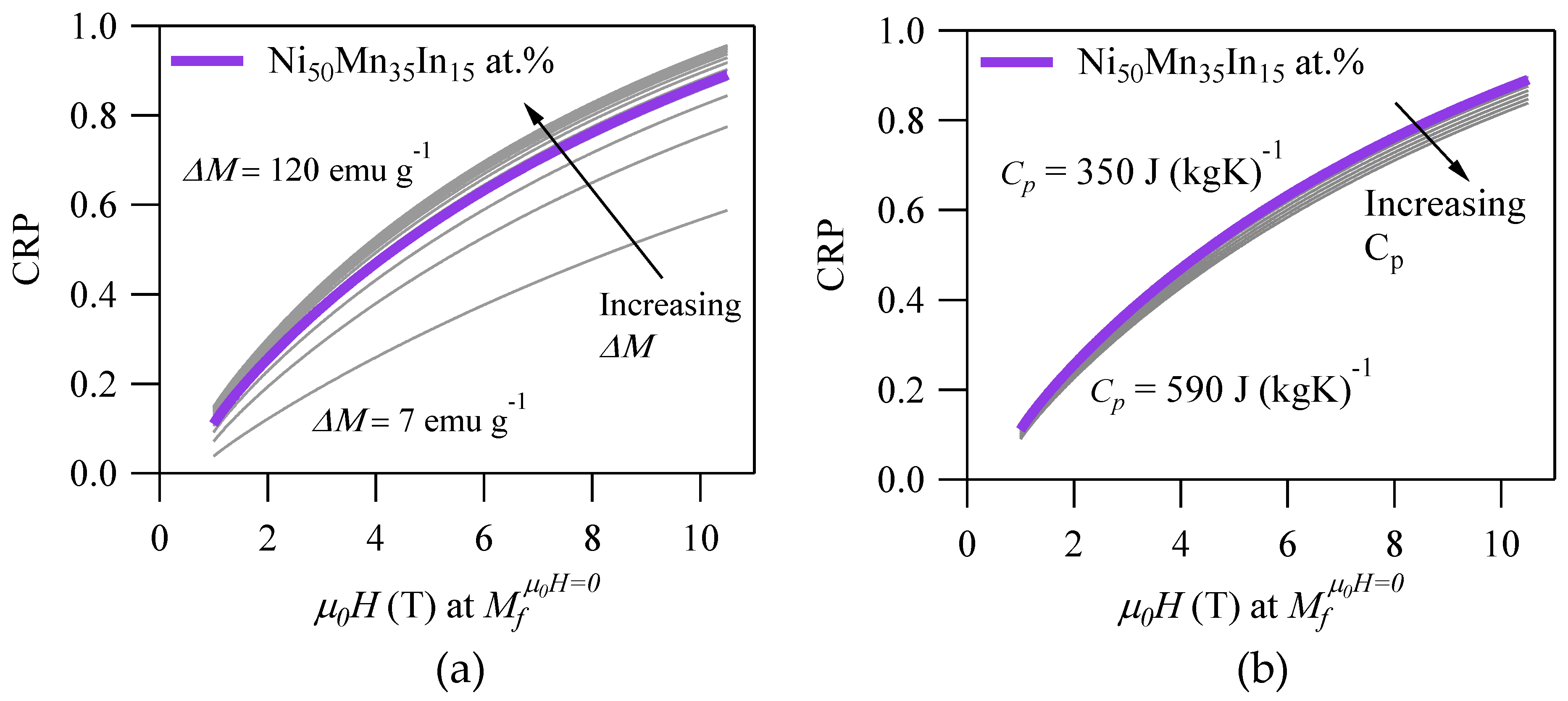
For instance,
Figure 4a depicts the CRP vs.
for various
within the bounds in
Table 2. From the figure, it is clear that the CRP would be reduced significantly for alloys that exhibit
< 27 emu·g
−1. In practice, this would eliminate MMSMAs that are characterized by a paramagnetic austenite from consideration for MCE applications. By decreasing
from 27 emu·g
−1 to only 7 emu·g
−1, the CRP would be reduced by 25% when cycling
. The CRP exhibited less sensitivity to
above 27 emu·g
−1, and therefore, this value should be used as a threshold when selecting materials for MCE applications.
Figure 4b depicts the CRP vs.
for various
. Since the
is present in only one term of the
in Equation (20), and the ratio of the highest to lowest values as given in
Table 2 is low (a factor of two times, compared to nearly 17 times for
), the effect to the CRP is minor. Nonetheless, lower values would obviously produce greater
and a higher
RC. Higher
would, in turn, increase
, which might decrease the CRP, because greater magnetic work would need to be applied to the material to generate the cooling effect. Thus, the CRP of an alloy may be increased by decreasing
, although the change is relatively small.
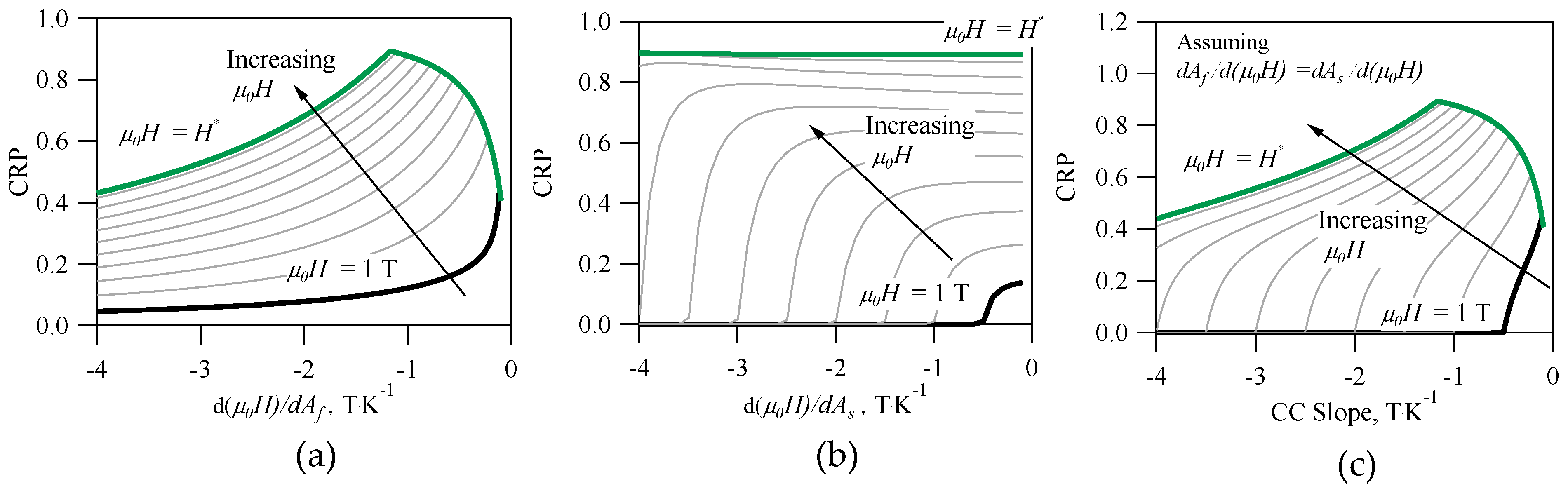
Finally,
Figure 5a–c depict the CRP vs. inverse CC slopes for an alloy with the same properties as the architype NiMnIn. The inverse CC slopes appear to have the greatest influence on the CRP out of all the material properties in Equation (25). This is not surprising, because the entropy change, or
in Equation (19), depends on the inverse CC slope. In
Figure 5a, the CRP is depicted as a function of
for
= 1, 2, 3, 4, 5, 6, 7, 8, 9, 10, and 10.5 Tesla. For the Ni
50Mn
35In
15 alloy,
= 10.5 T. As mentioned earlier,
was used to compute
,
, and the
RC in Equation (22); therefore, the influence of
on the CRP is highly nonlinear. Interestingly, the results in
Figure 5a suggest an optimum may exist in the CRP, which appears to be dependent on
. For example, if the cycled magnetic field was
= 2 T, a CRP of 0.61 would be achievable if
= −4.5 K·T
−1. If
= 5 T, a CRP of 0.79 would be achievable if
= −1.81 K·T
−1. Under the given framework, an absolute maximum in the CRP of 0.89 is attainable if
was applied to the Ni
50Mn
35In
15 alloy as long as
= −0.85 K·T
−1. The maximum CRP rapidly decreases if the magnitude of
is less −0.85 K·T
−1. Many, but not all, of the compositions in
Table 1 that exhibit a CRP of zero also exhibit a
with a magnitude less than −0.85 K·T
−1.
Similarly, the CRP vs.
was plotted in
Figure 5b for an alloy with materials properties matching those of Ni
50Mn
35In
15 at.%. The
parameter was only used in quantifying
, therefore affecting
for a given
. The
parameter does not appear to affect the maximum attainable CRP; however, the results in
Figure 5b can be used to determine acceptable
needed achieve a non-zero CRP.
In most literature, only one CC slope is reported, i.e., the thermodynamic equilibrium point of the forward (A-to-M) martensitic transformation, but in most MMSMAs, there are four separate CC slopes. In the case of the inverse MCE, we focus on the reverse (M-to-A) martensitic transformation, and therefore, the
and
slopes are the most important. Assuming the thermodynamic equilibrium from M-to-A at the
and
exhibit the same sensitivity to
, the CRP vs. the inverse CC slope would exhibit features from both
Figure 5a,b, as depicted in
Figure 5c. In
Figure 5c, non-zero CRP is attained at specific inverse CC slopes and
that also correspond to some CRP maximum.


