
Numerical Solution of Desiccation Cracks in Clayey Soils


Division of Civil & Building Services Engineering (CBSE), London South Bank University (LSBU), London SE1 0AA, UK
Encyclopedia 2022, 2(2), 1036-1058; https://doi.org/10.3390/encyclopedia2020068
Submission received: 22 April 2022
/
Revised: 15 May 2022
/
Accepted: 22 May 2022
/
Published: 24 May 2022
(This article belongs to the Collection Encyclopedia of Engineering)
Definition
:This entry presents the theoretical fundamentals, the mathematical formulation, and the numerical solution for the problem of desiccation cracks in clayey soils. The formulation uses two stress state variables (total stress and suction) and results in a non-symmetric and nonlinear system of transient partial differential equations. A release node algorithm technique is proposed to simulate cracking, and the strategy to implement it in the hydromechanical framework is explained in detail. This general framework was validated with experimental results, and several numerical examples were published at international conferences and in journal papers.
1. Introduction
Crack produced by desiccation in clayey soils is a problem that has implications in a wide range of ground-related fields. Geotechnical engineering, agriculture, mining, radioactive waste storage, tailings reservoirs, gravity dams, and public buildings are all affected by cracks due to desiccation [1,2,3,4,5].
The crack patterns that appear during desiccation are random, unique, and their development depends on multiple factors. Experimental approaches and numerical contributions have been made in the last 50 years [2,6,7,8,9,10,11,12,13,14,15,16,17,18,19,20,21,22,23]. Comprehensive state of the art was published in the last decade [12,24].
The process of cracking due to desiccation in clayey soils is difficult to treat numerically because the features involved are not well understood and they are dependent on one another. The process of initiation and evolution of the cracks includes a desiccation process first (a hydraulic process) and a process of shrinkage after (a mechanical process). The hydraulic and the mechanical components of the problem are both nonlinear processes. Most of the soil’s properties that affect the cracking process depend on the suction (see definition of suction in Equation (3)) or moisture content values. The process is hydromechanical and coupled. Adding to the complexity is the not-yet-well-understood soil–atmosphere interaction. The mineral composition of the clay as well as the salts dissolved in the water could play a role in the process, but this influence is beyond the scope of this hydromechanical formulation.
In the past, several approaches have been presented for dealing with this problem, with models available for each phase. There are numerical approaches in the literature based on the finite element method (FEM), the discrete element method (DEM), the distinct element method (DiEM), the mesh fragmentation technique (MFT), the lattice spring model (DLSM) [2,11,25,26,27,28,29,30,31], etc.
There is a model [32] that presents a relatively simple application of linear elastic fracture mechanics (LEFM) to simulate tension cracks in soils. In that work, however, the soil is not drying, and the fracture toughness can be determined in a relatively easy way at the laboratory for the convenient water content of the specimen. Commercial codes, such as FLAC® [33], based on the finite difference method have been applied for simulating the curling of a high-plasticity clay subjected to desiccation with no restrictions and with no cracks [11]. Rodríguez et al. [2] developed a one-dimensional hydromechanical approach to study the initiation of a crack during a desiccation process applied to mine wastes. The model proposed by Trabelsi et al. [25] takes into account the heterogeneity of the soil and uses as the main variable the porosity to study the initiation and propagation of cracks in thin samples. The distinct element method proposed by Amarasiri et al. [27] (Amarasiri et al., 2011) is an adaptation of the commercial code UDEC® [34] for analysing desiccation cracks in soils. This approach uses an interface element to simulate the cracks but does not calculate the flow in the porous media (the variation of water content with time needs to be known). The discrete element method (DEM) has been used for the simulation of crack desiccation in thin cylindrical specimens [26] using the commercial code PFC3D® [35] in which the variation of the stiffness and the tensile strength was taken into account and drying shrinkage was imposed on each aggregate at the micro-scale. The mesh fragmentation technique [28] uses high-aspect-ratio elements between the standard elements of a mesh making the model easily adapted to standard finite element programs. The lattice spring model DLSM is a two-phase bond model [29]. Finally, there have been several attempts to use simple models of particles connected by springs or viscoelastic Maxwell elements [36].
The classical theories of continuum mechanics, unsaturated soil mechanics, and the strength of materials and concepts in fracture mechanics are the preferable framework when studying problems such as this. The mathematical problem that emerges from the classical theories in this approach is resolved by the finite element method using material parameters obtained from laboratory tests in a controlled environment. Then, the approach is theoretical, experimental, and numerical (Figure 1).
In this entry, the flow in deformable porous media is resolved by the finite element method with a formulation [37]. A release-node technique is used to simulate the cracking process. The capabilities of the approach have been published recently [24,38]. In this approach, desiccation, shrinkage, and cracking are solved without imposing distribution or variation of water content. The system evolves from its initial conditions in suction and displacements first. After a while, the first crack appears when the tensile strength is reached at a point in the soil’s matrix. The release-node algorithm deals with the propagation of the cracks allowing changes in the suction at the boundaries at the new surfaces created by the cracks. Any other technique discussed above to tackle the cracking process can be implemented in the context of the general finite element hydromechanical model proposed here. The more complex the fracture mechanics approach is, the more parameters determined at the laboratory will be necessary and the more numerical instabilities will have to be resolved when simulating the process.
2. Mathematical Formulation and Numerical Solution for Desiccation Cracks in Clayey Soils
Although the three main physical processes involved in the formation of drying cracks (desiccation, shrinkage, and cracking) can be studied separately, to understand and model the process, it is necessary also to consider the interactions and couplings between them. Physically, the problem is coupled because the evaporation of water from the soil matrix produces matrix suction, and this matrix suction produces shrinkage and cracking. Shrinkage and cracking contribute to the desiccation process because deformation forces move the water out of the soil matrix and cracks produce new boundaries that water can use to evaporate.
Desiccation occurs because of a thermodynamical imbalance between the saturated soil mass and the environment (involving mainly temperature and relative humidity), leading to evaporation and water flow through the porous medium. When the process starts, the environment induces suction at the soil–air boundary because the relative humidity of the air is less than the relative humidity of the soil mass. For this reason, the suction is a boundary condition of the hydromechanical problem and the suction gradient in the soil specimen produces a flow of water through the porous medium towards the external surface, resulting eventually in evaporation, while in the soil’s pores an evaporation–condensation process occurs constantly. Desiccation is a non-adiabatic process because energy is needed for the evaporation. This energy comes from external pressures and high temperatures that, together with the soil’s shrinkage, produce changes of water pressure and of suction. This hydromechanical coupling shrinkage-flow is governed by several well-known physics laws: Darcy’s law relates the relative velocity between water and soil with the hydraulic gradient and describes the movement of air when the pores are interconnected; the air dissolution in water is governed by Henry’s law, and the diffusion of air in water is governed by Fick’s law. The soil temperature decreases during desiccation when the energy is taken from the soil. Under non-isothermal conditions, there are other effects, such as Soret’s thermal diffusion of water vapours in the air, because of pressure gradients produced by temperature gradients [39,40,41], vapor effusion, and Stefan’s flow [42].
When suction increases, capillary effects produce shrinkage, reducing the volume of the soil specimen and reduction of the void ratio. This may happen in saturated or unsaturated conditions. At the same time, the increasing suction gives consistency to the solid matrix and increases the stiffness and the tensile strength [15,43,44]. If the deformation is restricted, then, once the tensile strength is reached, cracking develops [9]. There are three types of restrictions to shrinkage: (1) boundary conditions in displacements or stresses (e.g., friction between different portions of soil or adherence with a soil container); (2) concentration of stresses in the soil mass; or (3) heterogeneity or impurities in the soil structure [45].
Desiccation cracks can appear in saturated and/or unsaturated conditions [12]. In fact, at the beginning of the process, the behaviour of the soils is more similar to a liquid with no tensile strength at all. Tensile strength develops because of the increment in suction when the soil acquires consistency. The water loss produces increment in suction that induces unidimensional vertical shrinkage, first, and a three-dimensional shrinkage when the soil becomes stiffer. The changes in the soil properties during the process induce a change in the boundary conditions at the contact between the soil and a container (e.g., loss of adherence or crack formation). Physically, cracking is a boundary condition problem, and, for this reason, a consistent approach must deal with this boundary condition more than facing the problem from the constitutive point of view.
The model presented here is developed in terms of two separated stress variables, suction and net stress, to have the main variables directly related to the experimental results. The consequence of this choice is that coupling of the hydraulic and mechanical problems is made through the material model, and the global system of equations obtained from the finite element method is non-symmetric. Although this is only one of different approaches that can be chosen regarding this topic [46], the numerical results obtained show the present election’s effectiveness.
In order to simplify the hydromechanical analysis, a mechanical constitutive model with a nonlinear elastic relation based on the stress state surface [47,48] is chosen. With this choice, the necessity of a complex stress point algorithm (plasticity model) can be avoided, and an explicit integration scheme can be used. Of course, other plastic models, such as Cam Clay, can be implemented within this general framework.
The hydraulic problem is relatively complex because of the highly nonlinear dependence of the properties and parameters on suction [7,12,49]. Although the hydromechanical analysis is at the core of the crack desiccation problem, it is crucial to have a solver for the simulation of crack initiation and propagation. Cracks are macroscopic discontinuities in the soil matrix that need to be implemented in the numerical formulation. In the present model, a release-node technique is used to simulate the initiation and propagation of a crack. This technique is relatively simple to implement and is effective to simulate the cracks induced by desiccation as is demonstrated in [38]. With this method, the tensile strength is the only parameter necessary to be determined in the laboratory. Although linear elastic fracture mechanics (LEFM) has been proposed as an alternative approach [2,32,50], the fracture parameters for soils are difficult to obtain in comparison, which is the reason why the strength of material approach is preferable.
The model presented here is based on classical theories in the context of geotechnical engineering and is consistent and relatively simple. This is preferable instead of adding additional numerical items to solve this already complex problem. However, complexity can be added gradually to include all the variables and factors that affect the physical process and the numerical results (non-isothermal processes, intrinsic and extrinsic factors, etc.).
2.1. Mathematical Formulation
In the formulation presented, the soil is assumed to be unsaturated during cracking, with negative (tensile) porewater pressure at the initial saturated or nearly saturated stage. This is convenient because conventional unsaturated soil mechanics can be used. The unsaturated soil framework allows setting up a desiccation simulation fixing hydraulic (suction) and mechanical (displacements) boundary conditions. Significant changes in hydraulic and mechanical properties that should be treated as material nonlinearities for consistent modelling are produced by changes in the degree of saturation [51]. This is particularity important in the desiccation problem because changes in volume (shrinkage) and stresses induced by the water loss in the soil mass are produced. There are three fundamental issues during the process of desiccation in soils: (1) volume change associated with water loss; (2) tensile and shear strength properties that depend on the saturation degree changes; and (3) hydraulic behaviour depending on suction or saturation degree [46].
To simplify the numerical analysis, at least regarding the mechanical constitutive relation, a nonlinear elastic model is chosen as an example in this entry. A set of parameters for this material model can be found in Appendix A and results of the model in 2D in Appendix B for Barcelona silty clay desiccated under controlled laboratory conditions [38]. This model is appropriate when the deformations are mainly volumetric, and the shear deformation does not have much relevance (suction is a spherical tensor that induces isotropic deformation). The hypotheses of the model include isothermal processes (the phases are at the same temperature and constant in time), small and slow deformations (infinitesimal quasi-static model), the medium is unsaturated and there are two fluid phases: liquid (water) and gas (dry air and water vapour), the pressure of air is constant and equal to zero (the air flows without resistance), and the state variables of the hydromechanical problem are the displacement of the soil matrix and the suction (tensile porewater pressure).
2.1.1. Mechanical and Hydraulic Constitutive Relations
To resolve the problem of desiccation cracks in clayey soils it is necessary to consider the next definitions and equations:
- Stress state variables.
- Stress–strain–suction relations.
- Stress–strain relation.
- Generalized Darcy’s law for unsaturated soils and permeability tensor.
- Water retention curve.
The concept of state surfaces [47,48] is chosen for the mechanical component of this model, allowing a simple implementation of a nonlinear elastic constitutive law. For the hydraulic component, the relation between suction and degree of saturation is modelled using the van Genuchten’s closed form expression, and the generalized Darcy’s law [52].
Stress State Variables
Historically, for unsaturated soils, an effective stress tensor () similar to the effective stress tensor for saturated soils was proposed [53], as shown in Equation (1):
In Equation (1), is the total stress tensor. The air and water pressure are, respectively, and , is a parameter that depends on the degree of saturation, the stress history, and the soil’s fabric, and is the identity tensor. In this formulation, the matrix suction and the net mean stress define the effective stress tensor through Equation (1). Other authors argue that it is better to work with two separate variables, the net stress and the suction that can be determined at the laboratory [54,55,56,57,58]. This latter approach is followed in this work.
The net stress (stress over the air pressure) and the suction are
Assuming small deformations, the Cauchy strain tensor is expressed as
where is the symmetric gradient operator and is the soil matrix displacement vector. is the symmetric gradient operator in matrix form when using Voigt’s notation.
Stress–Strain–Suction Relations
For oedometric and triaxial deformation and considering only a half-cycle of desiccation, which is the case of the desiccation process, a nonlinear elastic constitutive approach is enough to define the changes in volume and the development of stresses in the soil matrix. The state surfaces [47,48] are experimentally obtained in the laboratory (see Figure 2) and are an interpolation in the space. In this case, Equation (6) is used:
where is the void ratio increment, are state surface parameters calibrated from laboratory tests, and is a reference pressure to avoid logarithm indeterminacy.
Increments in net stresses and/or suction increase the void ratio, which is related to the volumetric deformation by
where is the volumetric deformation and the initial void ratio. In the desiccation problem, deformations occur because of the decrease of void ratio triggered by increments of suction (capillary effect).
Stress–Strain Constitutive Law
The general strain–stress relation must be written in differential form because of the nonlinearity of the material behaviour; Equation (8):
where is the fourth-order tangent stiffness tensor. The deformations are calculated by addition of a component due to the net stress plus a component due to the suction. Equation (9) considers, then, the additive deformation hypothesis:
In Equation (9), the parameter is the volumetric modulus and is the shear modulus of the soil matrix; the parameter is the volumetric modulus due to changes in suction; the factor is a fourth-order compliance tensor, and is a second-order tensor.
The net stress increments can be obtained from (9):
In Equation (10), , is the tangent stiffness tensor.
The compliance and stiffness tensors depend on the volumetric and shear modulus and . The suction tensor depends on the volumetric suction modulus . During the desiccation process, () are variables since the volumetric strain depends on the state surface of the soil. Combining Equations (6) and (7):
The total strain increment and then the volumetric strain can be decomposed into net strain and suction strain increments, and . Incrementally, this is
In Equation (12), and are the tangent moduli that depend on the mean net stress and on suction. Therefore
Moreover, is
Studying Equations (13) and (14) allow to see the relation between the tangent moduli and the volumetric strain:
The increment of the volumetric deformation, , during a time increment
, can be calculated from Equation (11):
Differentiating with respect to the mean net stress and suction :
The tangent elastic moduli can then be obtained from Equations (15) and (17) in terms of the state surface parameters , and the stress variables :
If the air pressure is assumed to be constant and equal to zero, , the elastic moduli can be calculated as in the formulas below:
For simplicity and because the deformation produced by the increment of suction is mainly volumetric, the Poisson’s ratio can be assumed constant. Additionally, a linear elastic relation between the shear and Young’s moduli can be adopted:
The volumetric deformation produced by changes of suction is then
and the stress–strain relation becomes
Finally, in matrix form, the stress–strain relation is
where is the tensor of deformations due to suction and it is spherical () and is the identity tensor. An isotropic nonlinear elastic material is defined by the stiffness tensor . In this constitutive law, volumetric and shear deformations are uncoupled.
Generalized Darcy’s Law for Unsaturated Soils and Permeability Tensor
The generalized Darcy’s law for unsaturated soils is
In Equation (24), is the velocity of Darcy vector; is the gradient of the porewater pressure; is a permeability tensor that changes with water saturation degree (); is the gravity vector; and is the water density.
The permeability tensor in terms of the intrinsic permeability is written as
In Equation (25), is the relative permeability and it is nondimensional. Its values are in the range 0 to 1. This parameter changes with the degree of saturation (here, , where is a constant). The parameter is the dynamic viscosity of water and it is temperature-dependent; is the intrinsic permeability tensor, which is a function of the porosity and of the viscosity and temperature of the fluid. Finally, is the unit weight of water, and is the hydraulic conductivity of the soil.
For cases where the hydromechanical coupling cannot be neglected, it is necessary to relate the saturated hydraulic conductivity to changes of porosity. An expression that can be used for that purpose is
where is the saturated hydraulic conductivity of reference at , and is the saturated hydraulic conductivity for porosity . In the last equation, is a material parameter. For saturated soils, .
Water Retention Curve
The van Genuchten function [59] is adopted in this formulation in order to relate changes between the degree of saturation and the suction when constant air pressure is considered:
where is a material parameter and is the air-entry value for the initial porosity , adopted as the reference value. Function considers the changes of porosity during desiccation and its effect in the water retention curve by means of a parameter . For non-deformable soils , because porosity is constant.
2.1.2. Governing Equations
The theoretical framework is defined using a multiphase approach where every phase (soil matrix, water, and air) fills up the entire domain and is known at the macroscopic level [60]. The process of desiccation is studied in unsaturated conditions considering the water to be in a tensile state of stress once the suction boundary condition has been defined for the hydromechanical problem. The global variables of the hydromechanical problem are the displacement vector of the soil matrix and the suction in the pores. The finite element method has been chosen for the discretisation in space and the finite differences method for the time discretisation of the problem.
The governing equations of this problem are
- Equilibrium equation of the solid particles.
- Balance equation of water.
Equilibrium Equations
In an unsaturated porous medium, the equilibrium equation in terms of total stresses is
Equation (28) is an elliptic partial differential equation where is the total stress tensor, is the net stress tensor, is the air pore pressure, is the average density of the multiphase medium (soil, water, and air), and is the gravity vector.
Assuming the air pressure is constant and equal to zero, , the stress state variables are and , and the equilibrium equation becomes
where the density of the multiphase medium is
where is the density of the solid particles, is the density of water, and is the degree of saturation.
Balance Equations
In an unsaturated porous medium, the fluid mass balance equation (or conservation of water mass) is written as follows:
which is a parabolic equation. Assuming water to be incompressible, the water density is constant:
Combining Darcy’s law, Equation (21), with the balance equation, the general flow equation is obtained:
Adding an additional term including water compressibility, which is usual in this type of problem, a diffusive term which stabilizes the numerical solution and permits dealing with quasi-incompressible and compressible problems is obtained:
where is the water compressibility coefficient.
Assuming that the increment of porosity is equal to the volumetric deformation (), and considering that in general and using the chain rule to evaluate , the following equation is obtained:
For desiccation problems, the saturation degree depends only on the porewater pressure by means of the water retention curve, . Then , and Equation (35) is simplified to
This problem is highly nonlinear because all variables depend on the porewater pressure which is the main unknown variable in this strong form of the hydraulic problem: , , . Also of interest are its gradient and temporal derivative, and, respectively, because they are needed to evaluate the increment of porosity, which is equivalent to the volumetric deformation. Finally, it is also necessary to evaluate the temporal derivative of the porosity, .
The initial and boundary conditions for the transient hydromechanical problem are specified in terms of displacements and of porewater pressure. The initial conditions are
where is the domain and its boundary; is the displacement field of the soil matrix; is the displacement field at the initial time ; and is the initial porewater pressure.
The Dirichlet boundary conditions for the hydromechanical problem are
where and are displacements and pore water pressures at the boundary of the domain.
The Newman’s stress boundary conditions for the hydromechanical problem are
where is the vector normal to the boundary; is the traction vector on the boundary; and is the following operator:
where are the components of the unit vector normal to the boundary.
Finally, the Newman’s flow boundary condition for the hydromechanical problem is
where is the flow perpendicular to the boundary.
2.2. Numerical Approach
This formulation is a one-phase flow in a deforming unsaturated porous media problem known as Richard’s problem [61].
2.2.1. Finite Element Approximation
The main variables and the ones that are unknown in the desiccation problem are the porewater pressure, , and the displacements in the soil matrix, . In the framework of the finite element method, the porewater pressure can be approximated by using the shape functions, , and the pressure, , in the nodes of an element. For a two-dimensional problem, the porewater is calculated as
where is the interpolated value of the porewater pressure. The variation with time of the porewater pressure is given by
Similarly, the displacement vector can be approximate at the nodes in a two-dimensional analysis by using the shape functions, , and the nodal displacements, :
The variation with time is
The incremental form with respect to time of the constitutive Equation (23) is expressed as
The displacement is related to the deformation by Equation [38], and after substituting (44), the following expression of the strain tensor is obtained:
Replacing Equations (43) and (47) in Equation (46):
The integral form of the equilibrium equation is
Replacing Equation (48) into Equation (49):
and considering that
and
The integral form of the hydraulic problem is
where are the weight functions. If the weight functions are such that , then
The u–p Formulation
The well-known u–p formulation [37] is adopted for solving the hydromechanical problem, where are the displacements and is the negative porewater pressure at the gauss points of the finite elements. Equations (50) and (54) are expressed as a non-symmetric system of partial differential equations:
where the tangent matrices of the stress-strain problem are
Stiffness matrix:
Coupling matrix:
Vector of nodal forces:
and the matrices of the flow problem are
Coupling matrix:
Compressibility matrix:
Permeability matrix:
Vector of nodal flow:
If matrix notation is used, the system of partial differential Equation (55) is
This form of hydromechanical problems in unsaturated soils is typical and can be found in the literature [62].
What is different in the derivation using separated variables is that the system is a non-symmetric system of equations because . The constitutive Equation (46) is the one that links the hydraulic variable (pore water pressure) with the mechanical variable (total stress).
Defining the next non-symmetric matrices:
and defining also
the compact form of the hydromechanical problem becomes
This is the differential equation that needs to be solved to simulate the desiccation shrinkage of unsaturated soils.
Time Integration of the Coupled Problem
In Equation (66), the unknown is , which is a vector that contains the unknown displacements and porewater pressures ( and , respectively) at the finite element mesh nodes. The time derivative can be expressed by the generalized trapezoidal method (generalized midpoint rule) as
and the value of the unknown at point is
Replacing Equations (67) and (68) in Equation (66) and multiplying both members by ,
Rearranging:
Placing the unknowns on the left side of the equation:
Equation (71) is a system of equations from which can be calculated from the values of and . This is an implicit method, and it is necessary to solve a system of equations in each time step. is the time interval between and , and the parameter varies between 0 and 1. Expanding Equation (71):
This is a non-symmetric system of nonlinear equations that can be solved using a coupled, staggered, or uncoupled scheme.
2.2.2. Release Node Algorithm
During a process of desiccation in clayey soil, cracking occurs at some point [2,7,12]. However, there are cases where desiccation produces shrinkage but not cracking, such as, for instance, in the curling produced in unrestricted tests [63]. For this problem, the formulation presented until here is directly applicable without any addition [24].
To simulate crack formation and propagation, there are three main variables that need to be established: the value of the stress at crack initiation (), the direction that the crack follows during propagation (), and the length of the crack when it is produced ()
In this approach, the tensile strength of the soil defines the stress value when cracking starts [59]. In the laboratory, the process of desiccation starts with the soil being a slurry with practically no tensile strength. After a while, the soil acquires consistency because of suction increments. During the process, the tensile strength increases first and after a while start decreasing (Figure 3a). This fact can be taken into account adopting an experimental expression to calculate the tensile strength as a function of the current suction, as proposed by [23] and shown in Equation (73).
where is the tensile stress in kPa and is the humidity content in %.
The equation and the parameters that relate the changes in the tensile strength with humidity will be different for different soils. Equation (73) is valid only for a clay from Barcelona, but the principle is general.
The direction of crack propagation can be taken as perpendicular to the maximum principal tensile stress. Since the soil matrix is discretized by a finite element mesh, the amount of propagation of a crack can be assumed to be equal to the length of the finite element. Cracks represent a change of boundaries because new crack surfaces (new boundaries) appear at each increment, and an appropriate algorithm needs to be implemented in the finite element code. Using this method, crack propagation is modelled as a sequence of temporal boundary-value problems. The discrete growing crack is assumed as a discontinuity. In the real soil, crack propagation occurs independently of a mesh. Failure of the material at the crack process zone is a continuous process. This is a limitation, but the simulation is good enough for certain purposes. In the model and in reality, when a new crack develops, new boundaries appear, and it becomes necessary to change the displacement and suction boundary conditions in the model. Then the geometry of the problem changes and it is necessary to solve the new problem to satisfy the equilibrium and balance conditions when the crack is growing.
At any point in the soil mass where the tensile stress reaches the tensile strength, a crack starts, and it propagates if the tensile strength is reached at the crack tip. Figure 3b shows the classical Griffith fracture criterion for a nonlinear elastic material [59]. This criterion is valid for the macroscopic scale, and when the tensile strength is reached, cracking starts instantaneously. There is no damage nor plastic zone at the crack tip. Despite the limitations of this technique in terms of what happens at the cracking area, it is easily implemented in the context of the finite element method and allows a first approach to cracking. The crack-opening mechanism must be established when the crack initiates and propagates. To simplify the analysis, only Fracture Mode I is taken into consideration in in this approach.
Release Node Algorithm
A simple technique to simulate the propagation of a crack in a finite element mesh consists of releasing a node that initially had a displacement boundary condition (Figure 4a) in the case of cracks at the soil–structure interface (e.g., soil in contact with a dam or wall). By releasing the node, after the condition is reached, a new geometric boundary is free to deform, and an elemental crack geometry is added to the model (Figure 4b). In Mode I, a crack propagates following a symmetry line perpendicular to the maximum principal tensile stress. In the case of a crack at the soil–structure interface, only the displacement boundary condition needs to be released. In addition, the new surface in contact with the environment will be subjected to the suction boundary condition and this needs to be added to the model (Figure 4d). In a more general case, when the crack propagation condition is reached on the surface of the soil, the node at the crack tip needs to be split into two nodes (Figure 4f,g) generating two new surfaces and propagating the crack a length equal to the element side . The new node generates a change in the node number list, node coordinates, and element connectivity, and therefore the mesh needs to be updated (this is an elemental re-meshing technique). The forces between the elements (or reactions, , at the boundary) that share the split node become zero after the opening and the system needs to be equilibrated. Some numerical problems can be expected because of the abrupt cancelling of these forces.
To avoid numerical instabilities, the unloading process is made gradually in several steps (Figure 4c,g).
The node release algorithm can be explained as follows:
- Fracture criterion is reached at a point in the soil matrix.
- Keep the external loads constant (suction profile for desiccation problems).
- Calculate reactions at the boundary, , or calculate equivalent forces that keep the split nodes together, .
- Delete the nodal restriction in the contour or split the nodes in the surface of the soil where the tensile strength was reached.
- Add reaction R at the released node (reaction in the contour) or forces in the node that was split.
- Reduce the force or F step by step to zero.
- Add suction on the new surface created by the crack and exposed to the environment.
- Once the model is in equilibrium, check whether the fracture criterion is reached at any other point of the geometry.
- If yes, go to step 3 to initiate again the release node algorithm.
- If no, continue the hydromechanical analysis.
When the crack propagation path is known, this technique is very useful and simple to implement. When desiccation is studied in the laboratory, the first cracks that appear are in the interphase between the soil and the containers, then, the first cracks directions and locations are known. For more arbitrary cracks, this technique is mesh-dependent but works relatively well if the mesh is dense enough. This method effectively calculates the stress state in the soil matrix during desiccation. This stress state is crucial for defining the initiation of the cracks and their propagation using any other alternative method to deal with the cracks.
Limitations of the Model
Several intrinsic factors define the direction of crack propagation: the tensile strength, the initial water content, anisotropy, imperfections, heterogeneity, impurities, the fracture toughness, the initial particle size, and the fabric in the field, just to mention the most important ones. If these intrinsic factors need to be added to the analysis, a more sophisticated fracture approach must be implemented in the context of the finite element hydromechanical model proposed here. Linear elastic fracture mechanics and a heterogeneous, anisotropic plastic material model should be implemented. The imperfections and impurities should be added to the geometry of the problem.
It is important to mention that the validity of the Darcy’s law, symmetry of the strain tensor, and invariability of the Poisson’s ratio are limitations of this model.
In this complex process, even the water density changes with temperature, salt content, permeability of the medium, etc. [64].
Aside from the geotechnical context of this entry, there are chemical, sedimentological, mineralogical, and petrological considerations that can be made to improve the model, adding the relevant parameters and physical laws. The necessary modifications and improvements of the model will depend on the area of interest and the practical application.
However, the formulation presented in this entry is general, so all these changes will be relatively simple to implement from the proposed framework. The challenge will be the determination of the material parameters and dealing with the numerical instabilities of the nonlinear material problem that every extra refinement will introduce to the formulation.
3. Conclusions and Prospects
In this entry, a mathematical formulation and a numerical solution for the analysis of desiccation cracking in clayey soils is presented. This model is hydromechanical and includes all the main variables and features that control the physical process of desiccation in clayey soils. The beauty of this approach is that it is based on fundamental principles. The unsaturated soils mechanics and strength of materials principles are used, avoiding the need for data obtained at the laboratory to force the system to behave as in reality. Once the initial conditions in suction and displacement are set, the system evolves until reaching a new state of equilibrium with the environment. The release node algorithm added to the hydromechanical core allows the study of at least a crack initiation and propagation as is shown in Appendix B.
The model offers a good balance between complexity and relatively simple implementation tools for the analysis of desiccation cracking in clayey soils. All the parameters that control the physical process can be easily determined from conventional experimental tests. The formulation is general and adaptable to more complex problems. The resulting approach helps to understand the process of desiccation cracking in soils.
This hydromechanical model without the cracking algorithm can be used for studying the curling process that soils show in the laboratory without cracks.
This model can be improved to take into consideration boundary effects such as the soil–atmosphere [65]. One way of achieving that is to simulate the fluid of the atmosphere in contact with the soil and its interaction.
The hydromechanical model can be modified to introduce more complex fracture mechanics approaches to have more control on the fracture process. Methods such as the mesh fragmentation technique can improve the treatment of multiple cracks and it can be added to the hydromechanical model presented here.
Heterogeneity and anisotropy can be added via the constitutive laws at a cost of having to determine more elastic parameters.
Imperfections can be added in the geometry or in the mesh.
If there is a need to study the process inside the pores, more sophisticated models can tackle the air dissolution in water governed by Henry’s law and the diffusion of air in water governed by Fick’s law. All these processes can be added at constitutive level using the same hydromechanical core and numerical solution.
If the temperature and chemical processes are relevant variables for a study, a thermal–chemical–hydromechanical formulation will be necessary. Adding the thermal component is relatively simple. The soil temperature decreases during desiccation when the energy is taken from the soil. Under non-isothermal conditions, there are other effects, such as Soret’s thermal diffusion of water vapours in the air, because of pressure gradients produced by temperature gradients, vapor effusion, and Stefan’s flow. All of these can be added to the formulation if necessary.
The hydromechanical core is essential to develop any other model to study the crack desiccation in clayey soils. For this reason, the mathematical formulation and the numerical solution is presented here in every single detail to allow researchers to implement it when necessary. To help with the implementation of the hydromechanical core, a set of parameters are included in Appendix A. Of course, these parameters need to be calibrated for every soil. Numerical examples can be found in previous publications of this author and a sequence of the simulation for a particular laboratory sample is presented in Appendix B. Since experimental validation is crucial for any model, results of experiments and comparison with the numerical approach are presented in Appendix C.
Additionally, the interaction between the soil and the atmosphere is crucial for the complete understanding of the process and for the moment is a topic being researched separately [65].
This model needs to be validated in three-dimensional studies [66] considering several types of soils to be properly validated for a wider range of soils and situations. This is indeed a live line of research of the author.
Funding
This research received no external funding.
Institutional Review Board Statement
Not applicable.
Informed Consent Statement
Not applicable.
Acknowledgments
Support from the Centre for Civil and Building Services Engineering (CCiBSE) at the School of the Built Environment and Architecture, London South Bank University is gratefully acknowledged.
Conflicts of Interest
The author declares no conflict of interest.
Appendix A. Set of Parameters for a Numerical Model for Barcelona Silty Clay

Table A1.
Water retention curve parameters for Barcelona silty clay.
| Void Ratio (e) | Porosity (n) | Dried Unit Weight γd (g/cm3) | fn = exp[−η(n − n0)] | λ | 1/(1 − λ) |
|---|---|---|---|---|---|
| 0.87 | 0.47 | 1.45 | 1.04 | 0.27 | 1.37 |
| 0.75 | 0.43 | 1.55 | 1.07 | 0.25 | 1.33 |
| 0.64 | 0.39 | 1.65 | 1.12 | 0.23 | 1.30 |
| 0.55 | 0.35 | 1.75 | 1.16 | 0.20 | 1.25 |
Table A2.
Parameters used in the numerical analysis of Barcelona silty clay.
| Mechanical Parameters | ||||||
|---|---|---|---|---|---|---|
| State surface parameters | (MPa) | Poisson Ratio | Tensile strength (MPa) | |||
(MPa) | ||||||
| −0.02 | −0.0025 | −0.000039 | 0.023 | 0.1 | 0.4 | 0.0035 |
| Hydraulic Parameters | ||||||
| Initial permeability (m/s) | Material parameter | Initial porosity | Material parameter | |||
| 9.27 × 10⁻¹⁰ | 25 | 0.6 | 3 | |||
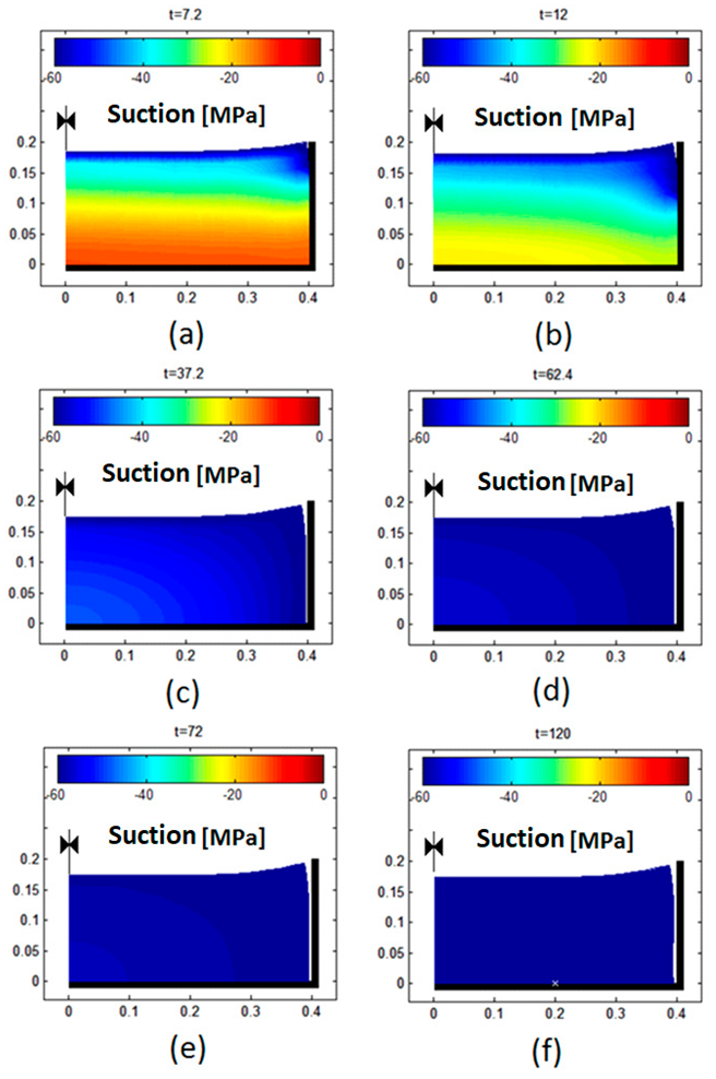
Appendix B. Numerical Results of the Model for Barcelona Silty Clay
Simulation of 120 days of desiccation on a cylindrical soil sample 80 cm in diameter and 20 cm height desiccated under controlled conditions. The figure shows the evolution of the suction in the radial section of the cylindrical sample and the propagation of a crack in contact with the container of the soil in the laboratory. (a) Suction and crack after 7 days of drying; (b) suction and crack after 12 days of drying; (c) suction and crack after 37 days of drying; (d) suction and crack after 62 days of drying; (e) suction and crack after 72 days of drying; (f) suction and crack after 120 days of drying. The results show the effectivity of the release node algorithm to simulate a cracking process by desiccation.
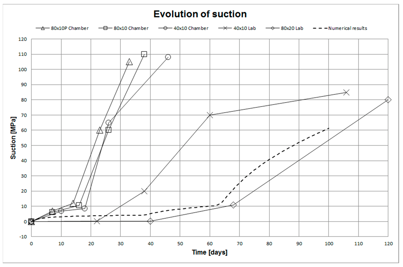
Appendix C. Comparison of Experimental and Numerical Results of the Model
Evolution of suction for different samples of 80/40 cm in diameter and 20/10 cm height in laboratory and environmental chamber conditions. The numerical simulation of radial cross-section 40 cm wide and 20 cm high is included to validate the model with the experiment.
References
- Rodríguez, R.L. Estudio Experimental de Flujo y Transporte de Cromo, Níquel Y Manganeso en Residuos de la Zona Minera de Moa (Cuba): Influencia del Comportamiento Hidromecánico. Ph.D. Thesis, UPC-BarcelonaTech, Barcelona, Spain, 2002. [Google Scholar]
- Rodríguez, R.L.; Sánchez, M.J.; Ledesma, A.; Lloret, A. Experimental and numerical analysis of a mining waste desiccation. Can. Geotech. J. 2007, 44, 644–658. [Google Scholar] [CrossRef]
- Tang, C.-S.; Shi, B.; Liu, C.; Zhao, L.; Wang, B. Influencing factors of geometrical structure of surface shrinkage cracks in clayey soils. Eng. Geol. 2008, 101, 204–217. [Google Scholar] [CrossRef]
- Justo, J.L.; Vázquez, N.J.; Justo, E. Subsidence in saturated-unsaturated soils: Application to Murcia (Spain). In Third International Conference on Unsaturated Soils; Jucá, J.F.T., de Campos, T.M.P., Marinho, F.A.M., Eds.; Balkema: Rotterdam, The Netherlands, 2002; pp. 845–850. [Google Scholar]
- Bronswijk, J.J.B. Modeling of water balance, cracking and subsidence in clay soils. J. Hydrol. 1988, 97, 199–212. [Google Scholar] [CrossRef]
- Kodikara, J.; Barbour, S.L.; Fredlund, D.G. Desiccation cracking of soil layers. In Unsaturated Soils for Asia; Rahardjo, H., Toll, D.G., Leong, E.C., Eds.; Balkema: Rotterdam, The Netherlands, 2000; pp. 693–698. [Google Scholar]
- Ávila, G. Estudio de la Retracción Y el Agrietamiento de Arcillas. Aplicación a la Arcilla de Bogotá. Ph.D. Thesis, UPC-BarcelonaTech, Barcelona, Spain, 2004. [Google Scholar]
- Chertkov, V.Y. Modelling cracking stages of saturated soils as they dry and shrink. Eur. J. Soil Sci. 2002, 53, 105–118. [Google Scholar] [CrossRef]
- Corte, A.; Higashi, A. Experimental Research on Desiccation Cracks in Soil; U.S. Army Materiel Command Cold Regions Research & Engineering Laboratory: Wilmette, IL, USA, 1960. [Google Scholar]
- Hu, L.B.; Hueckel, T.; Péron, H.; Laloui, L. Modeling Evaporation, Shrinkage and Cracking of Desiccating Soils. In Proceedings of the International Association for Computer Methods and Advances in Geomechanics (IACMAG), Goa, India, 1–6 October 2008; pp. 1083–1090. [Google Scholar]
- Kodikara, J.K.; Nahlawi, H.; Bouazza, A. Modelling of curling in desiccation clay. Can. Geotech. J. 2004, 41, 560–566. [Google Scholar] [CrossRef]
- Lakshmikantha, M.R. Experimental and Theoretical Analysis of Cracking in Drying Soils. Ph.D. Thesis, UPC-BarcelonaTech, Barcelona, Spain, 2009. [Google Scholar]
- Lakshmikantha, M.R.; Prat, P.C.; Ledesma, A. Characterization of crack networks in desiccating soils using image analysis techniques. In Numerical Models in Geomechanics X; Pande, G.N., Pietruszczak, S., Eds.; Balkema: Rotterdam, The Netherlands, 2007; pp. 167–176. [Google Scholar]
- Lakshmikantha, M.R.; Prat, P.C.; Ledesma, A. Image analysis for the quantification of a developing crack network on a drying soil. Geotech. Test. J. 2009, 32, 505–515. [Google Scholar]
- Lakshmikantha, M.R.; Prat, P.C.; Ledesma, A. Experimental evidences of size-effect in soil cracking. Can. Geotech. J. 2012, 49, 264–284. [Google Scholar] [CrossRef]
- Lakshmikantha, M.R.; Prat, P.C.; Ledesma, A. Evidences of hierarchy in cracking of drying soils. ASCE Geotech. Spec. Publ. 2013, 231, 782–789. [Google Scholar]
- Lau, J.T.K. Desiccation Cracking of Clay Soils. M.S. Thesis, University of Saskatchewan, Saskatoon, SK, Canada, 1987. [Google Scholar]
- Morris, P.H.; Graham, J.; Williams, D.J. Cracking in drying soils. Can. Geotech. J. 1992, 29, 263–277. [Google Scholar] [CrossRef]
- Nahlawi, H.; Kodikara, J. Laboratory experiments on desiccation cracking of thin soil layers. Geotech. Geol. Eng. 2006, 24, 1641–1664. [Google Scholar] [CrossRef]
- Péron, H.; Hueckel, T.; Laloui, L.; Hu, L.B. Fundamentals of desiccation cracking of fine-grained soils: Experimental characterisation and mechanisms identification. Can. Geotech. J. 2009, 46, 1177–1201. [Google Scholar] [CrossRef]
- Tang, C.-S.; Shi, B.; Liu, C.; Gao, L.; Inyang, H. Experimental Investigation of the Desiccation Cracking Behavior of Soil Layers during Drying. J. Mater. Civ. Eng. 2011, 23, 873–878. [Google Scholar] [CrossRef]
- Tang, C.-S.; Shi, B.; Liu, C.; Suo, W.-B.; Gao, L. Experimental characterization of shrinkage and desiccation cracking in thin clay layer. Appl. Clay Sci. 2011, 52, 69–77. [Google Scholar] [CrossRef]
- Vogel, H.J.; Hoffmann, H.; Roth, K. Studies of crack dynamics in clay soil. I: Experimental methods, results, and morphological quantification. Geoderma 2005, 125, 203–211. [Google Scholar] [CrossRef]
- Levatti, H.U. Estudio Experimental Y Análisis Numérico de la Desecación en Suelos Arcillosos. Ph.D. Thesis, UPC-BarcelonaTech, Barcelona, Spain, 2015. Available online: https://www.tdx.cat/handle/10803/299202#page=1 (accessed on 12 January 2022).
- Trabelsi, H.; Jamei, M.; Zenzri, H.; Olivella, S. Crack patterns in clayey soils: Experiments and modelling. Int. J. Numer. Anal. Methods Geomech. 2012, 36, 1410–1433. [Google Scholar] [CrossRef]
- Sima, J.; Jiang, M.; Zhou, C. Modeling desiccation cracking in thin clay layer using three-dimensional discrete element method. Proc. Am. Inst. Phys. 2013, 1542, 245–248. [Google Scholar]
- Amarasiri, A.L.; Kodikara, J.; Costa, S. Numerical modelling of desiccation cracking. Int. J. Numer. Anal. Methods Geomech. 2011, 35, 82–96. [Google Scholar] [CrossRef]
- Sánchez, M.; Manzoli, O.L.; Guimarães, L.N. Modeling 3-D desiccation soil crack networks using a mesh fragmentation technique. Comput. Geotech. 2014, 62, 27–39. [Google Scholar] [CrossRef]
- Gui, Y.; Zhao, G.F. Modelling of laboratory soil desiccation cracking using DLSM with a two-phase bond model. Comput. Geotech. 2015, 69, 578–587. [Google Scholar] [CrossRef]
- Yan, C.; Luo, Z.; Zheng, Y.; Ke, W. A 2D discrete moisture diffusion model for simulating desiccation fracturing of soil. Eng. Anal. Bound. Elem. 2022, 138, 42–64. [Google Scholar] [CrossRef]
- Nikolic, M. Discrete element model for the failure analysis of partially saturated porous media with propagating cracks represented with embedded strong discontinuities. Comput. Methods Appl. Mech. Eng. 2022, 390, 27. [Google Scholar] [CrossRef]
- Lee, F.H.; Lo, K.W.; Lee, S.L. Tension crack development in soils. J. Geotech. Eng. ASCE 1988, 114, 915–929. [Google Scholar] [CrossRef]
- ITASCA. FLAC3D: Fast Lagrangian Analysis of Continua in Three Dimensions; Version 2.0 Manual; Itasca Consulting Group: Minneapolis, MN, USA, 1997. [Google Scholar]
- ITASCA. UDEC: Distinct-Element Modeling of Jointed and Blocky Material in 2D; Itasca Consulting Group: Minneapolis, MN, USA, 2017. [Google Scholar]
- ITASCA. PFC3D: Particle Flow Code in Three Dimensions; Version 3.0 Manual; Itasca Consulting Group: Minneapolis, MN, USA, 2003. [Google Scholar]
- Musielak, G.; Sliwa, T. Modeling and Numerical Simulation of Clays Cracking During Drying. Dry. Technol. 2015, 33, 1758–1767. [Google Scholar] [CrossRef]
- Zienkiewicz, O.C.; Chan, A.H.C.; Pastor, M.; Paul, D.K.; Shiomi, T. Static and Dynamic Behaviour of Soils: A Rational Approach to Quantitative Solutions. I. Fully Saturated Problems. Proceedings of the Royal Society of London Series A. Math. Phys. Sci. 1990, 429, 285–309. [Google Scholar]
- Levatti, H.U.; Prat, P.C.; Ledesma, A. Numerical and experimental study of initiation and propagation of desiccation cracks in clayey soils. Comput. Geotech. 2019, 105, 155–167. Available online: https://openresearch.lsbu.ac.uk/item/865wv (accessed on 12 January 2022). [CrossRef]
- Platten, J.K. The Soret Effect: A Review of Recent Experimental Results. J. Appl. Mech. 2006, 73, 5–15. [Google Scholar] [CrossRef]
- Ludwig, C. Diffusion zwischen ungleich erwwa”rmten orten gleich zusammengestzter lo”sungen. Sitz Ber. Akad. Wiss. Wien. Math.-Naturw. Kl. 1856, 20, 539. [Google Scholar]
- Soret, C. Sur l’état d’équilibre que prend au point de vue de sa concentration une dissolution saline primitivement homohéne dont deux parties sont portées à des températures différentes. Ann. Chim. Phys. 1881, 22, 293–297. [Google Scholar]
- Mitrovic, J. Josef Stefan and his evaporation–diffusion tube—the Stefan diffusion problem. Chem. Eng. Sci. 2012, 75, 279–281. [Google Scholar] [CrossRef]
- Varsei, M.; Miller, G.A.; Hassanikhah, A. Novel approach to measuring tensile strength of compacted clayey soil during desiccation. Int. J. Geomech. 2016, 16, D4016011. [Google Scholar] [CrossRef]
- Lakshmikantha, M.R.; Prat, P.C.; Tapia, J.; Ledesma, A. Effect of moisture content on tensile strength and fracture toughness of a silty soil. In Unsaturated Soils: Advances in Geo-Engineering; Toll, D.G., Augarde, C.E., Gallipoli, D., Wheeler, S.J., Eds.; CRC Press/Balkema: Leiden, The Netherlands, 2008; pp. 405–409. [Google Scholar]
- Hueckel, T. On effective stress concept and deformation in clays subjected to environmental loads: Discussion. Can. Geotech. J. 1992, 29, 1120–1125. [Google Scholar] [CrossRef]
- Sheng, D. Review of fundamental principles in modelling unsaturated soil behaviour. Comput. Geotech. 2011, 38, 757–776. [Google Scholar] [CrossRef]
- Matyas, E.L.; Radhakrishna, H.S. Volume change characteristics of partially saturated soils. Géotechnique 1968, 18, 432–448. [Google Scholar] [CrossRef]
- Lloret, A.; Alonso, E.E. State surfaces for partially saturated soils. In Proceedings of the XI International Conference on Soil Mechanics and Foundation Engineering, San Francisco, CA, USA, 12–16 August 1985; pp. 557–562. [Google Scholar]
- Barrera, M. Estudio Experimental del Comportamiento Hidro-Mecánico de Suelos Colapsables. Ph.D. Thesis, UPC-BarcelonaTech, Barcelona, Spain, 2002. [Google Scholar]
- Konrad, J.-M.; Ayad, R. An idealized framework for the analysis of cohesive soils undergoing desiccation. Can. Geotech. J. 1997, 34, 477–488. [Google Scholar] [CrossRef]
- Gens, A.; Sánchez, M.; Sheng, D. On constitutive modelling of unsaturated soils. Acta Geotech. 2006, 1, 137–147. [Google Scholar] [CrossRef]
- Van Genuchten, M.T. Closed-form equation for predicting the hydraulic conductivity of unsaturated soils. Soil Sci. Soc. Am. J. 1980, 44, 892–898. [Google Scholar] [CrossRef]
- Bishop, A.W. The principles of effective stress. Tek. Ukebl. 1959, 106, 859–863. [Google Scholar]
- Burland, J.B. Some aspects of the mechanical behaviour of partly saturated soil. In Moisture Equilibrium and Moisture Changes in Soils Beneath Covered Areas; Butterworths: Sydney, Australia, 1965; pp. 270–278. [Google Scholar]
- Bishop, A.W.; Blight, G.E. Some aspects of effective stress in saturated and partly saturated soils. Géotechnique 1963, 13, 177–197. [Google Scholar] [CrossRef]
- Blight, G.E. A study of effective stresses for volume change. In Moisture Equilibrium and Moisture Changes in Soils Beneath Covered Areas; Butterworths: Sydney, Australia, 1965; pp. 259–269. [Google Scholar]
- Aitchison, G.D. Soil properties. In Proceedings of the 6th International Conference on Soil Mechanics and Foundation Engineering, SMFE, Montreal, QC, Canada, 8–15 September 1965; pp. 319–321. [Google Scholar]
- Jennings, J.; Burland, J.B. Limitations to the use of effective stress in partly saturated soils. Géotechnique 1962, 12, 125–144. [Google Scholar] [CrossRef]
- Griffith, A.A. The phenomenon of rupture and flow in solids. Philos. Trans. Roy. Soc. Lond. 1921, 221, 163–198. [Google Scholar]
- Lewis, R.W.; Schrefler, B.A. The Finite Element Method in the Static and Dynamic Deformation and Consolidation of Porous Media, 2nd ed.; Wiley: Hoboken, NJ, USA, 1998. [Google Scholar]
- Richards, L.A. Capillary conduction of liquids through porous mediums. Physics 1931, 1, 318–333. [Google Scholar] [CrossRef]
- Schrefler, B.A.; Simoni, L.; Majorana, C.E. A general model for the mechanics of saturated-unsaturated porous materials. Mater. Struct. 1989, 22, 323–334. [Google Scholar] [CrossRef]
- Nahlawi, H.; Kodikara, J. Experimental observations on curling of desiccating clay. In Third International Conference on Unsaturated Soils; Jucá, J.F.T., de Campos, T.M.P., Marinho, F.A.M., Eds.; Balkema: Rotterdam, The Netherlands, 2004; pp. 553–556. [Google Scholar]
- Ledesma, A. Cracking in desiccating soils. In Proceedings of the 3rd European Conference on Unsaturated Soils, E-UNSAT, Paris, France, 12–14 September 2016. [Google Scholar]
- Cui, Y. Soil-atmosphere interaction in earth structures. J. Rock Mech. Geotech. Eng. 2022, 14, 35–49. [Google Scholar] [CrossRef]
- Zhuang, Z.; Zhu, C.; Tang, C.S.; Xu, H.; Shi, X.; Mark, V. 3D characterization of desiccation cracking in clayey soils using a structured light scanner. Eng. Geol. 2022, 299, 106566. [Google Scholar]
Figure 1.
A theoretical, numerical, and experimental approach to the desiccation crack problem in clayey soils.
Figure 1.
A theoretical, numerical, and experimental approach to the desiccation crack problem in clayey soils.
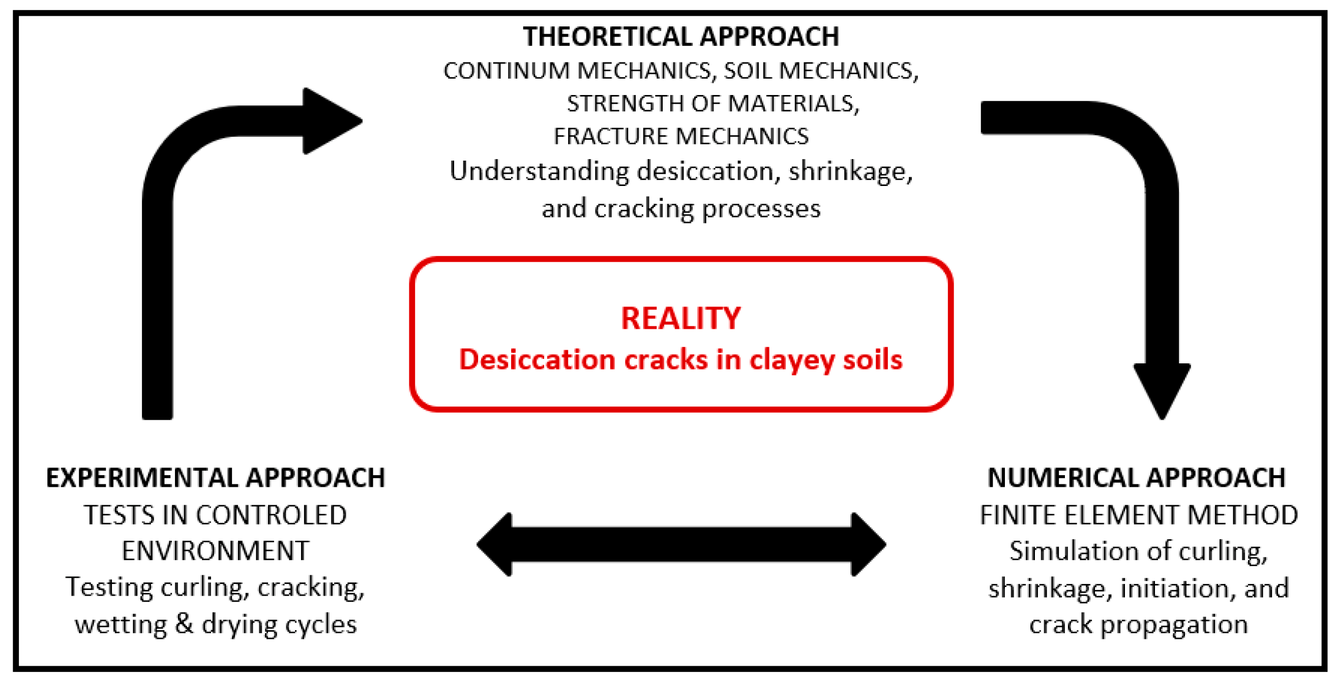
Figure 2.
State surfaces.
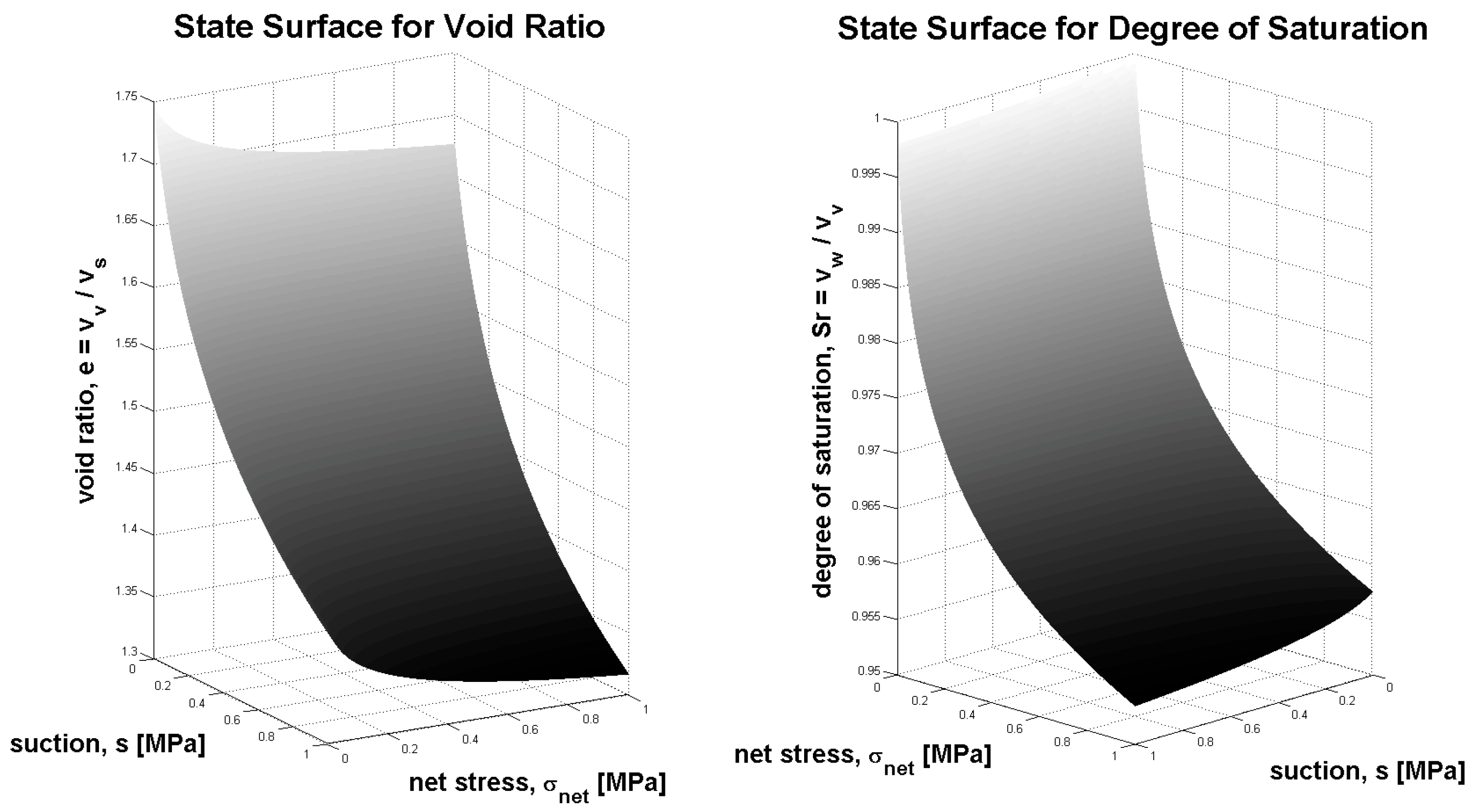
Figure 3.
Crack initiation criteria: (a) tensile strength, moisture-content-dependent [12]; (b) traditional strength of material failure criteria [59].

Figure 4.
Release node algorithm for a contour crack and a crack starting in the middle of the soil surface. Contour crack case: (a) starting scheme in a contour, (b) equivalent starting scheme after reaching the cracking criteria, (c) reaction reduction and application of new suction condition, (d) new contour condition scheme with crack propagated. General crack case: (e) initial conditions, (f) nodes are split and equivalent forces applied, (g) reduction of equivalent forces, (h) new contour condition scheme with crack propagated.
Publisher’s Note: MDPI stays neutral with regard to jurisdictional claims in published maps and institutional affiliations. |
© 2022 by the author. Licensee MDPI, Basel, Switzerland. This article is an open access article distributed under the terms and conditions of the Creative Commons Attribution (CC BY) license (https://creativecommons.org/licenses/by/4.0/).
Share and Cite
MDPI and ACS Style
Levatti, H.U. Numerical Solution of Desiccation Cracks in Clayey Soils. Encyclopedia 2022, 2, 1036-1058. https://doi.org/10.3390/encyclopedia2020068
AMA Style
Levatti HU. Numerical Solution of Desiccation Cracks in Clayey Soils. Encyclopedia. 2022; 2(2):1036-1058. https://doi.org/10.3390/encyclopedia2020068
Chicago/Turabian StyleLevatti, Hector U. 2022. "Numerical Solution of Desiccation Cracks in Clayey Soils" Encyclopedia 2, no. 2: 1036-1058. https://doi.org/10.3390/encyclopedia2020068