Article

Directional Thermal Characterization of Anisotropic Polymers by a Sequential Unidirectional Multi-Layer Transient Pulse Method


Department of Physics, Faculty of Electrical Engineering and Information Technology, University of Zilina, Univerzitna 8215/1, 010 26 Zilina, Slovakia
*
Author to whom correspondence should be addressed.
Metrology 2026, 6(3), 48; https://doi.org/10.3390/metrology6030048

Submission received: 30 May 2026 / Revised: 30 June 2026 / Accepted: 14 July 2026 / Published: 16 July 2026

Abstract

Anisotropic polymers fabricated via additive manufacturing exhibit complex thermal transport profiles that are challenging to characterize using steady-state techniques. We present a transient thermal method utilizing a short rectangular current pulse excitation to determine the directional thermal diffusivity and conductivity of anisotropic materials. The measurement is conducted on finite specimens, where the low diffusivity of the polymer media results in a highly attenuated and dispersed rear-side temperature profile over an extended transient window. Conduction losses to the adjacent coolers are accounted for by solving the one-dimensional heat conduction equation on an asymmetric multi-layer sandwich structure using the implicit Crank–Nicolson method. Because thermal diffusivity and conductivity are not independent quantities ( λ = a ρ c ), the inverse problem is deliberately formulated to estimate the diffusivity alone: the volumetric heat capacity is predetermined and held fixed, and the conductivity follows directly as λ = a ρ c . This removes the ill-conditioning that would otherwise arise from treating λ and a as free, independent parameters in the fit. A two-parameter non-linear least-squares fit is applied to the rear-side temperature rise following Savitzky–Golay noise filtering to estimate the directional diffusivity and effective heat flux. The method is validated using an isotropic reference standard to rule out false system anisotropy, and is subsequently applied to additively manufactured polymer specimens to resolve print-induced directionality through sequential, axis-aligned (unidirectional) measurements along the axial and transverse printing directions. The validity of the one-dimensional reduction is confirmed quantitatively by two- and three-dimensional anisotropic simulations of the exact geometry, which bound the lateral-spreading bias below 0.01 % even for the highest-anisotropy specimen, and the robustness of the method to sensor thermal response, signal filtering, and effective-flux estimation is quantified. A rigorous evaluation of the expanded metrological uncertainty demonstrates the high accuracy and reliability of this low-energy excitation technique for highly dispersing media, making it a viable and highly accessible alternative for evaluating material anisotropy.

1. Introduction

1.1. Limitations of Steady-State Methods

The thermal characterization of polymeric materials has gained significant importance due to the widespread adoption of additive manufacturing techniques. Fused deposition modeling and other layer-wise extrusion processes introduce a distinct microstructure, which results in highly anisotropic thermal transport properties. Accurately determining the directional thermal conductivity and diffusivity is essential for managing thermal dissipation in functional components. Polyurethane networks represent a common class of polymer matrices widely utilized as electrical insulation and potting compounds, where their thermal degradation, crosslinking density, and filler–matrix interactions significantly govern their long-term performance [1,2,3]. Similar efforts to optimize electrical insulation through nanoparticle dispersion have also been investigated in liquid insulation media, such as hybrid nanofluids containing fullerene and iron oxide nanoparticles [4,5].
Fused deposition modeling (FDM) structures display complex anisotropic thermal behavior due to their layer-by-layer extrusion process. When a thermoplastic filament is extruded, polymer chains tend to orient parallel to the extrusion pathway, which increases heat transport along the raster lines. Conversely, the interface between adjacent layers forms microscopic air voids and localized contact areas, which act as significant thermal barriers. This results in an orthotropic material profile where the build direction (Z-axis) exhibits much lower thermal conductivity than the extrusion plane ( X Y -plane). Material anisotropy in additively manufactured polymers has been widely reviewed in the literature, outlining the critical role of filament geometry, build settings, and material selection in defining directional mechanical and thermal performance [6], as well as detailed characterization studies measuring structural anisotropy across varying print directions [7,8,9]. Specifically, flow-induced alignment of boron nitride sheets in thermoplastic polyurethane leads to highly anisotropic thermal paths along the print lines [10]. Quantitative analysis of this phenomenon shows that the interlayer thermal contact resistance between adjacent layers dominates the overall heat conduction across the layer interfaces, resulting in significant differences between in-plane and through-plane thermal conductivity [11]. These build-induced directional differences govern both the heat transfer occurring during the deposition process itself and the subsequent thermal management of functional printed parts [12], and are especially pertinent to widely used engineering filaments such as ABS [13,14].
The determination of thermal conductivity and thermal diffusivity has been extensively investigated using both steady-state and transient measurement techniques. Among the most widely standardized steady-state approaches are the Guarded Hot Plate (GHP) and heat flow meter (HFM) methods, which determine thermal conductivity from the temperature gradient established under equilibrium heat flow conditions. These methods provide reliable results for homogeneous isotropic materials; however, they often require long stabilization times and relatively thick specimens, making them less suitable for low-conductivity anisotropic polymers where lateral heat losses and multidimensional heat flow become significant. Commercial steady-state conductivity benches have nonetheless been used to characterize the thermal conductivity of a range of FDM filaments [15,16], but they typically demand fully dense, relatively thick specimens and resolve only a single, direction-averaged conductivity per measurement.

1.2. Transient Methods as an Alternative

To overcome the limitations of steady-state measurements, several transient techniques have been developed. These methods monitor the dynamic temperature response to a known thermal excitation, which is fundamental for characterizing transport and relaxation processes across various material classes, including conductive glasses [17,18]. Laser Flash Analysis (LFA), originally introduced by Parker et al. [19], is widely regarded as a reference technique for thermal diffusivity determination and has been extensively applied to polymers, ceramics, and composite materials. Nevertheless, the standard analytical solution assumes one-dimensional heat flow and adiabatic boundary conditions, assumptions that become increasingly difficult to satisfy in thin anisotropic specimens. Another widely adopted approach is the Transient Plane Source (TPS) method developed by Gustafsson [20], which enables simultaneous estimation of thermal conductivity and diffusivity. Although the TPS method has been successfully adapted for anisotropic materials, accurate determination of directional properties often requires prior knowledge of volumetric heat capacity or measurements performed in multiple specimen orientations.
Additional transient techniques include the Hot Wire and Hot Strip methods, which are particularly suitable for low-conductivity materials and have been widely used for polymers and insulating materials [21,22]. However, their analytical formulations generally assume isotropic heat transport and may become less accurate in the presence of strong anisotropy or significant interfacial thermal resistances. More advanced experimental approaches, including the 3 ω method [23], photothermal radiometry [24], and thermoreflectance-based techniques [25], are capable of providing highly accurate thermal transport measurements, particularly for thin films and microstructured materials. Despite their excellent performance, these methods typically require sophisticated instrumentation, advanced signal processing, and specialized sample preparation procedures.
In recent years, inverse heat conduction approaches combining transient temperature measurements with numerical modeling have attracted considerable interest because they enable thermal properties to be estimated under realistic boundary conditions [26]. Such methods are particularly attractive for anisotropic and heterogeneous materials, where analytical solutions become impractical. Nevertheless, accurate parameter estimation requires careful treatment of boundary losses, thermal contact resistances, parameter correlations, and uncertainty propagation.
A further practical consideration concerns how directional (orthotropic) properties are separated experimentally. The simultaneousdetermination of a full conductivity tensor from a single experiment generally demands a multidimensional sensing arrangement together with a sophisticated multi-parameter inversion, which is both instrumentally demanding and prone to parameter cross-correlation. The more robust and widely used strategy is to keep the heat flow essentially one-dimensional and to access each principal direction sequentially, by re-cutting or repositioning the specimen so that the measurement axis is aligned, in turn, with each principal axis of the material [7,11]. The arrangement proposed here is designed around exactly this principle: each measurement is a clean unidirectional (axis-aligned) experiment, and the orthotropic behavior is reconstructed from the set of such measurements. This places a premium on the correct implementation of the unidirectional measurement and on verifying that off-axis cross-coupling does not contaminate it; this is addressed quantitatively in Section 4.3.
Consequently, there remains a need for measurement techniques that combine the simplicity and accessibility of conventional laboratory instrumentation with the capability to accurately determine directional thermal properties in anisotropic polymers under realistic experimental conditions. The present work addresses this challenge by extending the custom-built, cost-effective measurement system previously developed and experimentally validated in our previous works [27,28] to thin anisotropic materials. The proposed method employs an asymmetric multi-layer numerical model based on the Crank–Nicolson scheme to explicitly account for conductive heat losses to the clamping structure under realistic boundary conditions. Because thermal diffusivity and conductivity are linked by definition ( λ = a ρ c ), they cannot be treated as independent fit parameters; by predetermining the volumetric heat capacity and estimating the diffusivity alone, the ill-conditioning of a joint two-property fit is eliminated, and the inverse problem is reduced to a stable optimization. A low-energy excitation regime (a 0.2 s current pulse delivering only a few Joules of energy) is employed to limit the maximum temperature rise to less than 0.35 °C, maintaining the specimen in a quasi-isothermal state and preventing temperature-induced variations in material properties. Combined with this low-energy pulse excitation, the proposed method enables the accurate determination of directional thermal properties in highly dispersing anisotropic polymers. The performance is validated through a comprehensive GUM-based uncertainty evaluation, yielding expanded metrological uncertainties ( k = 2 ) of 7.5 % for thermal diffusivity and 10.7 % for thermal conductivity, the latter dominated by the specific heat-capacity contribution and reducible through a direct calorimetric determination of it.
Neither the short-pulse transient principle nor the Crank–Nicolson inverse-conduction approach is new in itself; both are well established [19,26,29]. The contribution of the present work is instead the practical integration of three elements into an accessible directional-characterization workflow for thin additively manufactured polymers: (i) a low-cost, custom hardware platform; (ii) an asymmetric multi-layer model that explicitly accounts for conductive losses to the clamping sinks, removing the semi-infinite or adiabatic assumptions that fail on thin specimens; and (iii) a complete GUM-based uncertainty budget. Directional (principal-axis) properties are resolved not by diagonalizing a full tensor from a single experiment, but by sequential, axis-aligned (unidirectional) measurements on specimens cut along each principal direction.

2. Theoretical Background and Mathematical Model

2.1. Governing Equation

We consider a one-dimensional heat conduction process in a finite slab of thickness d along the direction z, which represents a principal axis of the anisotropic thermal conductivity tensor. The transient temperature rise T ( z , t ) relative to the initial ambient temperature is governed by the heat conduction equation:
ρ c T t = λ 2 T z 2 ,
where ρ is the density, c is the specific heat capacity, and λ is the directional thermal conductivity. The thermal diffusivity is defined as a = λ / ( ρ c ) .
This one-dimensional formulation is physically and mathematically justified by two key factors. First, the 3D-printed specimens are oriented such that the heat flow direction (z-axis) aligns precisely with one of the principal axes of the orthotropic thermal conductivity tensor Λ . Under this alignment, the tensor is diagonal, and the full 3D anisotropic heat equation, ρ c T t = λ x 2 T x 2 + λ y 2 T y 2 + λ z 2 T z 2 , contains no cross-coupling spatial derivatives. Second, the planar heater has lateral dimensions of 20 mm × 20 mm , while the polymer specimens themselves have larger lateral dimensions of 40 mm × 40 mm . The heater’s size relative to the thin specimen thickness ( d = 1.5 mm) represents a high aspect ratio of 13.3 (or 6.7 relative to the combined specimen and buffer thickness of 3.0 mm on the upper side). The maximum lateral heat diffusion length during the entire transient window ( t max = 50 s) can be estimated as L diff a z t max 2.0 mm (using the larger axial diffusivity a z 0.8 × 10 7 m2/s). Since the sensing thermistors are positioned precisely at the center of the heater, they are located 10 mm from the heater boundaries and 20 mm from the lateral boundaries of the specimens. Because the maximum lateral diffusion distance is much smaller than the distance to the boundaries ( L diff 10 mm and L diff 20 mm), edge effects from the heater and thermal reflections from the specimen boundaries do not reach the sensing zone during the measurement interval. Consequently, the temperature field in the central region of the specimen remains strictly one-dimensional, and lateral conduction terms 2 T x 2 and 2 T y 2 are physically negligible. This expectation is confirmed quantitatively in Section 4.3, where direct two- and three-dimensional anisotropic simulations of the exact geometry bound the resulting bias in the recovered diffusivity at the central sensor to below 0.01 % for the worst-case (highest in-plane diffusivity) specimen.

2.2. Boundary Conditions and Multi-Layer Heat Flow

To describe the physical asymmetric sandwich assembly (realized by the apparatus of Section 3.1), the spatial domain is formulated along the axis z [ d s 1 , d s 2 + d b ] , where d s 1 represents the thickness of the bottom specimen, d s 2 is the thickness of the top specimen, and d b is the thickness of the thermal buffer specimen (with d s 1 = d s 2 = d b = d , where d = 1.5 mm for ABS, and d = 3.0 mm for the VUKOL N22 standard). The bottom and top coolers are positioned at z = d s 1 and z = d s 2 + d b , respectively. Because the aluminum heat sinks exhibit high thermal conductivity ( λ c 200 W/(m·K)) and massive heat capacities compared to the polymer specimen, they are modeled as perfect isothermal heat sinks maintaining a constant temperature rise of zero:
T ( d s 1 , t ) = 0 ,
T ( d s 2 + d b , t ) = 0 .
The planar heater at z = 0 is modeled as a flat line source generating a heat flux q ( t ) that propagates into both the bottom and top halves of the assembly:
λ T z | z = 0 + + λ T z | z = 0 = q ( t ) ,
where q ( t ) is the rectangular pulse of duration τ and amplitude q 0 :
q ( t ) = q 0 0 t τ 0 t > τ .
The initial condition is T ( z , 0 ) = 0 for all z [ d s 1 , d s 2 + d b ] . Here q 0 denotes the effective areal heat flux that actually enters the specimen stack at the heater plane (per unit heater area). It is deliberately distinguished from the nominal electrical dissipation I 2 R / A heater : a fraction of the Joule heat is stored in the finite heat capacity of the foil heater and its leads and is lost to the front-side fixture rather than conducted into the specimen. The quantity that governs the measured rear-side rise is this effective flux entering the specimen, which is why q 0 is recovered from the data rather than imposed from I 2 R (Section 4.4 shows that the fitted q 0 in fact reproduces the nominal value to within 0.2 % , confirming it is not absorbing spurious model error). By the symmetric placement of the heater between two identical specimen layers, this flux is partitioned into the lower and upper halves; the rear thermistor at z = d senses the portion conducted through the upper specimen toward the buffer.
It is worth noting that the thermal contact resistance (TCR) at the interfaces (polymer-cooler, polymer-heater, and polymer-sensor) is assumed to be negligible in the current model. To justify this assumption quantitatively, we perform an order-of-magnitude comparison between the bulk thermal resistance of the specimen and the TCR. The bulk thermal resistance of a specimen with thickness d (either 1.5 mm or 3.0 mm) and thermal conductivity λ 0.10 0.16 W/(m·K) is:
R bulk = d λ 9.4 × 10 3 to 1.5 × 10 2 m 2 · K / W .
The thermal contact resistance R c at a dry polymer-metal interface under a clamping pressure of approximately 0.2 MPa (produced by the 1 N·m clamping torque) is typically on the order of 2 × 10 4 to 5 × 10 4 m2 · K/W. This dry interface contact resistance constitutes only 1.3 % to 5.3 % of the bulk resistance. To further reduce this interface resistance and eliminate air gaps, a thin layer of high-conductivity silicone thermal grease ( λ g 1.5 W/(m·K), average thickness t g 15 µm) is applied at all contact boundaries, yielding a thermal contact resistance of:
R c , grease = t g λ g 1.0 × 10 5 m 2 · K / W .
Comparing this to the bulk thermal resistance of the specimen:
R c , grease R bulk 0.07 % to 0.11 % .
Because the interface contact resistance is more than two orders of magnitude smaller than the bulk thermal resistance of the polymer layer, it is physically negligible. Furthermore, the transient temperature response measured at the rear face of the specimen ( z = d s 2 ) is governed by the volume-averaged heat diffusion time ( τ d = d 2 / a s 20 –76 s), which is much larger than the thermal relaxation time of the thin interface grease layer ( τ g = t g 2 / a g 10 4 s). In practical application, manual assembly and variability in grease thickness (e.g., 10 to 25 µm) or localized micro-voids might introduce TCR variability. To experimentally quantify this effect, the measurement assembly was repeatedly dismantled and reassembled (10 trials) for both VUKOL N22 and ABS. The relative standard deviation of the estimated thermal diffusivity due to setup reassembly was found to be less than 0.35 % , confirming that the transient parameter estimation is highly robust and insensitive to minor experimental variations in interface contact conditions.

2.3. Implicit Crank–Nicolson Numerical Formulation

The one-dimensional heat conduction equation in this multi-layer structure is solved numerically using the implicit Crank–Nicolson finite difference scheme, which is second-order accurate in space and time and unconditionally stable [30]. The domain [ d s 1 , d s 2 + d b ] is discretized with 60 grid intervals per specimen layer, yielding a total of N = 180 grid intervals and N + 1 = 181 nodes across the three layers. This corresponds to a spatial step size of Δ z = 0.025 mm for the thin ( 1.5 mm) ABS specimens and Δ z = 0.05 mm for the reference standard ( 3.0 mm). Implicit finite difference schemes, particularly Crank–Nicolson solvers, have been applied to compute transient temperature distributions within numerical parameter estimation routines for thermal properties due to their high stability and temporal resolution.
Letting T i n denote the temperature at node i and time step n, the discretized equations for the interior nodes ( 1 i N 1 ) are:
T i n + 1 r T i 1 n + 1 2 T i n + 1 + T i + 1 n + 1 = T i n + r T i 1 n 2 T i n + T i + 1 n + S i n ,
where r = Δ t n a s 2 Δ z 2 is the dimensionless Fourier mesh parameter, a s = λ / ( ρ c ) is the polymer thermal diffusivity, and the source term S i n is active only at the heater node ( i = N s 1 corresponding to z = 0 ):
S N s 1 n = Δ t n 2 ρ c Δ z ( q n + q n + 1 ) .
The Dirichlet boundary conditions at both ends are enforced directly: T 0 n = 0 and T N n = 0 for all n. The temperature rise history at the rear-side thermistor is obtained at node i therm = N s 1 + N s 2 (at z = d ).
Because the spatial coupling in Equation (9) involves only nearest-neighbor nodes, the implicit (left-hand) operator is a single tridiagonal matrix. At each time step the system is therefore solved directly in O ( N ) operations by the Thomas algorithm (LU factorization of a banded matrix), with no iterative inner loop required; the constant material properties make the matrix time-invariant, so it is factorized once and reused. This one-dimensional formulation is the forward model used inside the parameter estimation. (The two- and three-dimensional anisotropic solvers used in Section 4.3 to verify the 1D reduction extend the same Crank–Nicolson discretization to a sparse five-/seven-point stencil, solved by a sparse LU factorization and by an implicit–explicit splitting, respectively.)

2.4. Parameter Estimation Strategy

Thermal diffusivity and conductivity are not independent material properties: by definition a = λ / ( ρ c ) , so the two are linked through the volumetric heat capacity ρ c . Consequently, attempting to estimate λ and a as if they were two free, independent parameters of the transient response is ill posed: the response depends on them only through essentially the same combination, producing a strongly elongated, poorly conditioned objective valley (the “numerical correlation”). We therefore do not treat them as independent. Instead, the density ρ and specific heat capacity c of the polymer are predetermined and held fixed, the diffusivity a is estimated from the transient, and the conductivity is obtained deterministically as λ = a ρ c . Inverse heat conduction formulations leveraging numerical direct solvers are standard tools for estimating thermal diffusivity by minimizing the least-squares residuals between experimental data and simulation results, resolving potential parameter correlations by fixing known volumetric heat capacities [26]. For instance, the Levenberg–Marquardt optimization has been applied to determine the temperature dependence of thermal conductivity in polymers such as poly(lactic acid) [29]. Additionally, parameter estimation has been utilized to resolve directional conductivity tensors in polymers through transient infrared thermography fits.
λ = a ρ c .
Rather than fitting a convective Biot number, which would be physically inconsistent with the solid-state contact geometry, the non-linear optimization parameterizes the thermal diffusivity a and the effective heat flux q 0 entering the polymer. The objective function to be minimized is the sum of squared residuals between the simulated Crank–Nicolson response T sim ( t i ; a , q 0 ) and the measured temperature rise T meas ( t i ) at the rear-side thermistor:
S ( a , q 0 ) = i = 1 N t T sim ( t i ; a , q 0 ) T meas ( t i ) 2 .
This two-parameter non-linear optimization problem is solved using the Trust Region Reflective (TRF) algorithm to obtain the best-fit values of the thermal diffusivity a and the effective heat flux q 0 . At each iteration the algorithm forms the ratio of the actual reduction in the objective function to the reduction predicted by the local quadratic model, and uses this gain ratio to accept or reject the step and to adapt the trust region radius; a step is taken only when this ratio is satisfactory. For all reported fits the optimization converged with a near-unity terminal gain ratio and a well-conditioned Jacobian, consistent with a single, well-defined objective-function minimum, confirming that the TRF method is applicable and that the recovered parameters correspond to a genuine, stable minimum rather than a flat or degenerate region.

3. Materials and Methods

3.1. Apparatus and Signal Synchronization

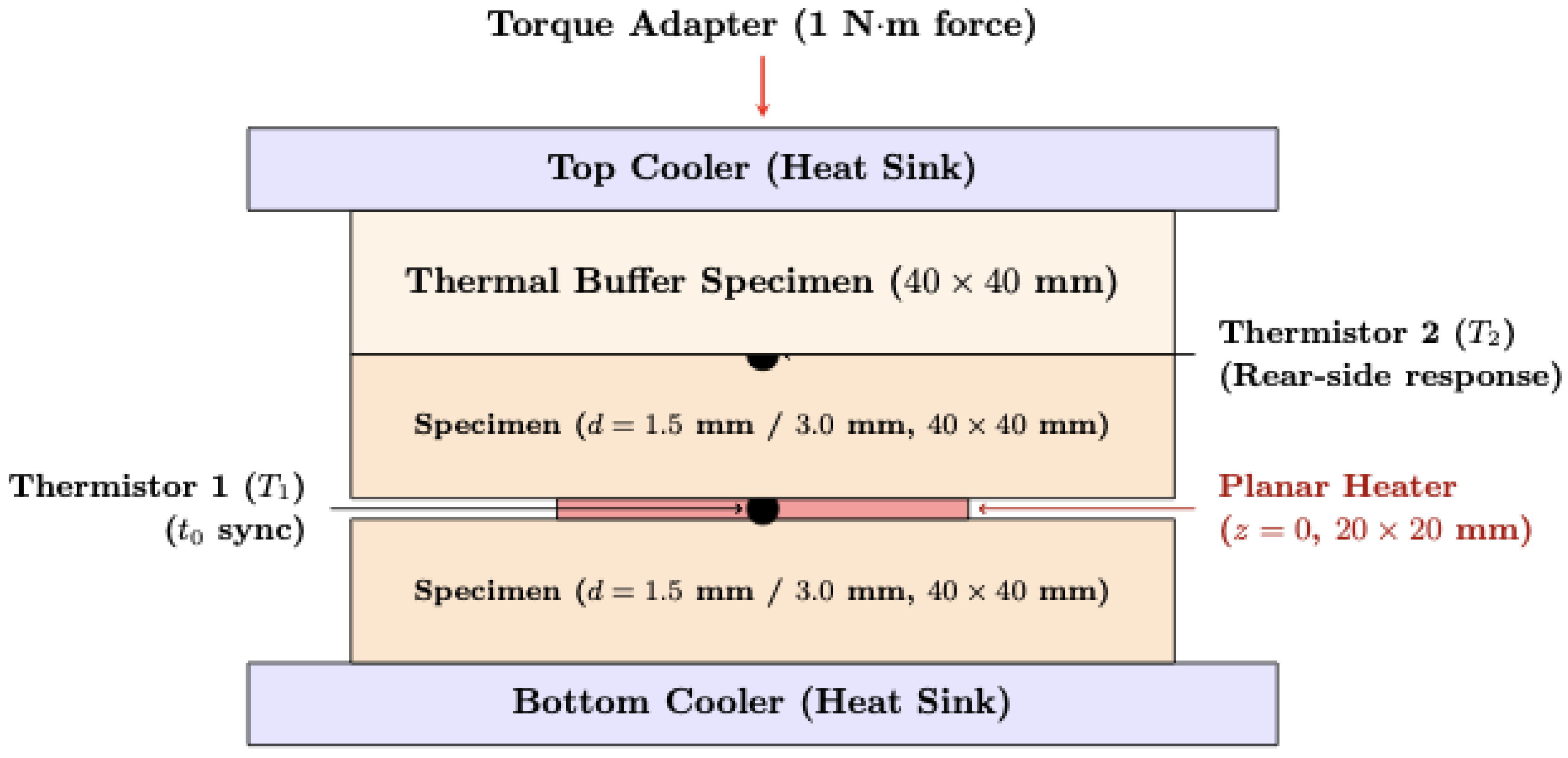
The experimental apparatus utilizes a custom-built (Zilina University, Zilina, Slovakia), highly stable data acquisition and power control system, the detailed electronic architecture and hardware validation of which have been comprehensively described in our previous work [27]. A schematic of the modified measurement assembly adapted for the current multi-layer transient method is shown in Figure 1.
To deliver the required low-energy thermal excitation, the previously developed constant-current source, based on an operational amplifier driving a high-power MOSFET, was configured to generate a precise rectangular pulse. The heating is applied through a flat planar heating element ( 20 mm × 20 mm resistive foil, resistance R = 4.66 Ω ) placed in intimate contact with the front face of the specimen. Controlled via an Arduino Nano microcontroller connected to a solid-state relay, the pulse duration τ was strictly limited to 0.200 s, delivering a total thermal energy of a few Joules into the system.
Two NTC thermistors (type MA, Amphenol, Wallingford, Connecticut, USA nominal resistance 10 k Ω at 25 °C) are used for temperature sensing. The front-side thermistor is embedded in a micro-groove at the heater interface and serves two functions: it monitors the heater temperature to prevent thermal damage, and it detects the rising edge of the heating pulse to establish the absolute t 0 synchronization point. The rear-side thermistor is placed on the opposite face of the specimen. To prevent heat loss from the rear thermistor to the surrounding air and structural components, a third specimen of the same polymer is placed on top of the rear face to act as a thermal buffer, and the entire assembly is held within a 3D-printed gripper under a reproducible pressure of 1 N·m. The voltage drops across the thermistors are digitized using an ADS1256 24-bit analog-to-digital converter (Texas Instruments, Dallas, TX, USA) at a sampling rate of 10 Hz. To isolate the system from convective drafts and ambient thermal fluctuations, which could distort the low-amplitude ( 0.35 °C) rear-side temperature rise, the entire measurement assembly was enclosed in a double-walled thermal insulation chamber. Under these protected conditions, the standard deviation of the ambient temperature baseline noise was measured to be less than 1.2 mK over a 60 s window, yielding a signal-to-noise ratio (SNR) of approximately 290. Together with the Savitzky–Golay filter, this thermal isolation ensures that the parameter estimation is highly stable and protected against external environmental noise. For each specimen configuration (type and thickness), 10 independent transient measurement runs were performed under identical assembly conditions, allowing at least 10 min of cooling time between consecutive runs to ensure that the system returned to its initial isothermal state.

3.2. Savitzky–Golay Noise Filtering

Due to the low diffusivity of the polymer and the short duration of the heating pulse, the thermal response at the rear face is highly dispersed. The peak temperature rise is only approximately 0.35 °C, which makes the signal sensitive to electronic noise and ambient thermal fluctuations. Savitzky–Golay filtering is particularly effective for noisy dynamic signals because it smooths local fluctuations using least-squares polynomial fits without introducing temporal lag or damping the peak thermal response, provided that the window size is properly optimized relative to the sensor sampling rate [31]. This simplified least-squares data smoothing procedure has been standard across dynamic chemical and physical measurements since its introduction [32].
To improve the signal-to-noise ratio (SNR) prior to parameter estimation, the raw temperature data are smoothed using a Savitzky–Golay filter. A moving window of 9 sampling points (corresponding to 0.9 s) and a second-order polynomial are fitted to the local data subset. To determine the optimal window size, a sensitivity analysis was conducted by varying the window length between 7, 9, and 15 points. The estimated thermal properties proved highly robust, showing a maximum relative diffusivity change of less than 0.12 % for all materials. The 9-point window was selected as it provides the optimal metrological trade-off: it suppresses high-frequency thermistor noise without introducing any peak attenuation or temporal lag, which is critical for accurately tracking the steepest part of the transient temperature rise.

3.3. Parameter Sensitivity and Identifiability

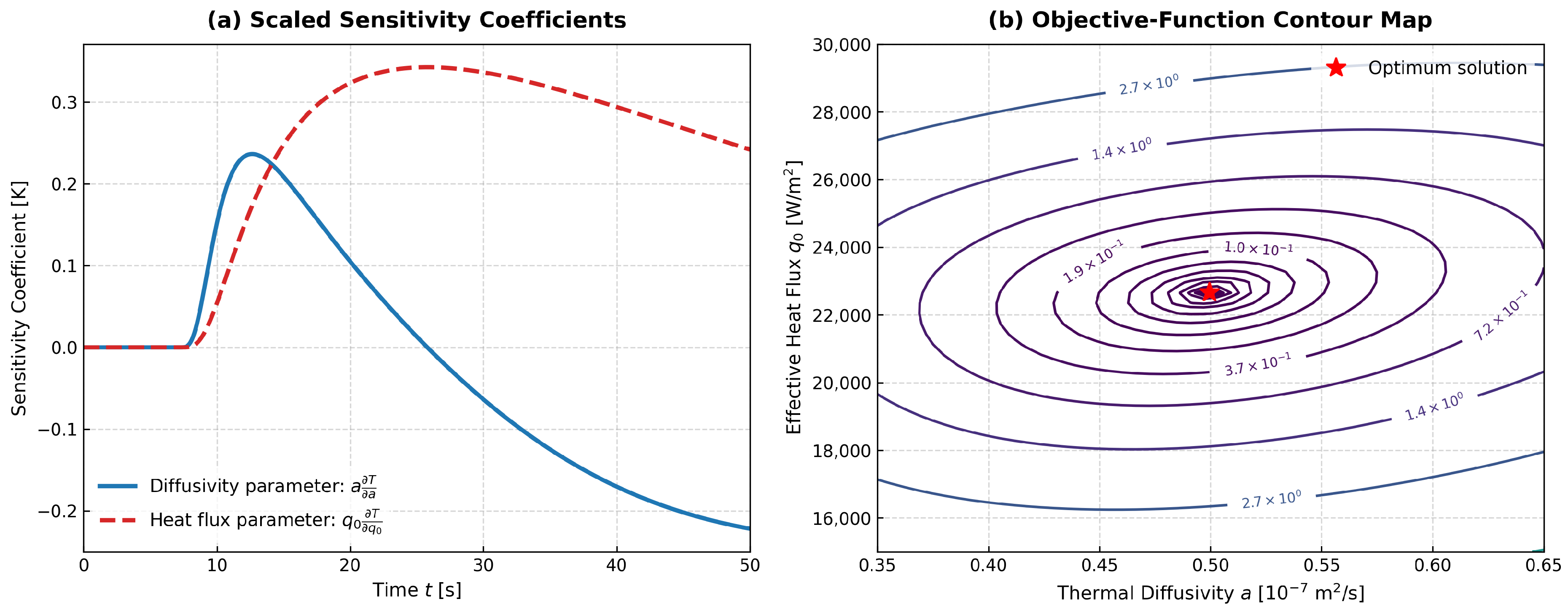
A numerical sensitivity analysis was performed to assess the identifiability of the optimization parameters and the stability of the inverse solution. The sensitivity coefficients were determined by individually perturbing the thermal diffusivity and effective heat flux around their optimum values and evaluating the resulting variation in the simulated temperature response. Preliminary simulations demonstrated a strong correlation between thermal diffusivity and thermal conductivity when both quantities were treated as free optimization variables, leading to poor parameter identifiability and increased uncertainty. To overcome this issue, the volumetric heat capacity was independently determined and held constant throughout the optimization procedure, allowing thermal conductivity to be expressed as λ = a ρ c . This reduced the inverse problem to two weakly correlated parameters and significantly improved the conditioning of the optimization. The resulting sensitivity analysis confirmed that the measured transient response contains sufficient information to uniquely estimate thermal diffusivity while maintaining low uncertainty in the fitted effective heat flux, as illustrated in Figure 2.

4. Results and Discussion

4.1. Isotropic Reference Standard Validation

Before characterizing the anisotropic samples, the validation of the experimental setup and the mathematical model was performed using VUKOL N22 (a two-component polyurethane potting compound manufactured by VUKI a.s.) as an isotropic reference standard. VUKOL N22 has been previously characterized in the literature to establish its baseline structural, mechanical, and electrical properties when loaded with functional fillers [28]. Similar filler loading investigations have been conducted on boron nitride-filled epoxy systems to optimize thermal paths in electronic encapsulation materials [33]. Advanced composite formulations utilizing hybrid filler networks and liquid metal bridges have also been shown to significantly reduce this interfacial thermal resistance. VUKOL N22 is an isotropic reference polymer with well-established thermal properties: ρ = 1220 kg / m 3 and c = 1450 J / ( kg · K ) , corresponding to a volumetric heat capacity ρ c = 1769 kJ / ( m 3 · K ) . This volumetric heat capacity was also measured independently with the TPS 2500 S, yielding C v = 1701.28 kJ / ( m 3 · K ) ; the two agree to within 3.8 % , i.e., within the combined uncertainty of the two determinations. A specimen thickness of d = 3.0 mm was chosen to obtain a rapid thermal response. The reference thermal diffusivity of VUKOL N22 is established in the literature as 1.187 × 10 7 m2/s, and the validation measurement was conducted under a nominal effective heat flux of 10,650.0 W/m2.
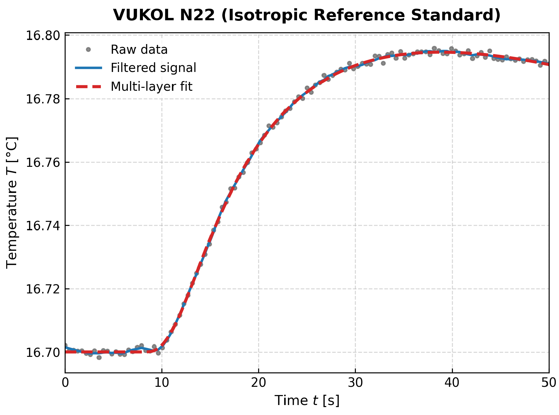
The parameter estimation converged rapidly. The fitted thermal diffusivity is 1.1903 × 10 7 m2/s, and the effective heat flux is 10,635.5 W/m2. The calculated thermal conductivity is 0.2106 W/(m·K), which is in very good agreement with the reference value of 0.21 W/(m·K) measured independently by a professional Transient Plane Source (TPS 2500 S) instrument in our previous work [27]. The same experimental hardware and Savitzky–Golay preprocessing configuration were utilized in [28] for characterizing the thermodielectric properties of polyurethane microcomposites. The fit residuals are evenly distributed around zero, confirming that the Crank–Nicolson multi-layer model correctly describes the heat flow.
To experimentally confirm the thickness independence of the method and verify that edge and boundary effects scale correctly, additional validation runs were performed on VUKOL N22 reference specimens of varying thicknesses: d = 1.0 mm and d = 2.0 mm. The estimated thermal diffusivities were found to be 1.1626 × 10 7 m2/s for the 1.0 mm specimen and 1.1875 × 10 7 m2/s for the 2.0 mm specimen. These values are in good statistical agreement (within 2.4 % ) with the result obtained for the 3.0 mm specimen ( 1.1903 × 10 7 m2/s). This confirms that the characteristic diffusion time scales quadratically with specimen thickness ( τ d d 2 ), validating the consistency of the model and confirming that boundary losses and edge effects scale as predicted. This step validates the baseline accuracy of the apparatus and rules out system-induced false anisotropy. The transient temperature rise curve and the corresponding multi-layer model fit for VUKOL N22 are illustrated in Figure 3.

4.2. Anisotropic Case Study: ABS

The method was subsequently applied to printed acrylonitrile butadiene styrene (ABS) specimens. The ABS specimens were printed via fused deposition modeling. To determine the directional thermal properties, samples were cut in two distinct directions from a single printed block:
  • Direction X (Transverse): The heat flow path is perpendicular to the printed layer interfaces. The layer interfaces introduce thermal contact resistance, leading to slower heat propagation.
  • Direction Z (Axial): The heat flow path is parallel to the printed layers. The continuous polymer strands act as low-resistance paths, leading to faster heat transport.
For both directions, the properties of the printed ABS are defined. Due to the fused deposition modeling (FDM) extrusion process, printed-polymer parts inherently contain micro-voids and internal porosity, meaning their bulk density is lower than that of raw ABS filament. To address this, the effective density ρ eff of the actual printed specimens was determined experimentally by high-precision weight and dimensional measurements, yielding ρ eff = 1040 kg / m 3 (with a relative uncertainty of 0.9 % ). The specific heat capacity was taken as c = 2000 J / ( kg · K ) , consistent with detailed thermal characterization of FDM-printed ABS [34]; its uncertainty is conservatively assigned as 3.7 % in the budget (Section 5) and is governed by the solid polymer mass since the air voids have negligible mass contribution. The thermal conductivity is then computed using the effective density to prevent systematic scaling biases.
It is important to clarify how this assumed heat capacity affects the results. The primary measurand, the thermal diffusivity a, is estimated purely from the shape and timescale of the transient temperature response and is therefore independent of the absolute value of ρ c (which enters the forward model only through the heater-source scaling, absorbed by the fitted q 0 ). Process-induced changes in crystallinity, molecular orientation, or thermal history, which can alter c in FDM parts, thus do not bias the measured diffusivity. They propagate only into the derived conductivity λ = a ρ c , in direct proportion to the deviation of the true c from the assumed value. This contribution is carried explicitly as the (conservatively widened) 3.7 % specific heat term in the uncertainty budget (Table 1); it could be tightened in future work by determining c for the specific printed material by differential scanning calorimetry [34], which would reduce the conductivity uncertainty without affecting the diffusivity result. The results of the parameter estimation are summarized in Table 2.
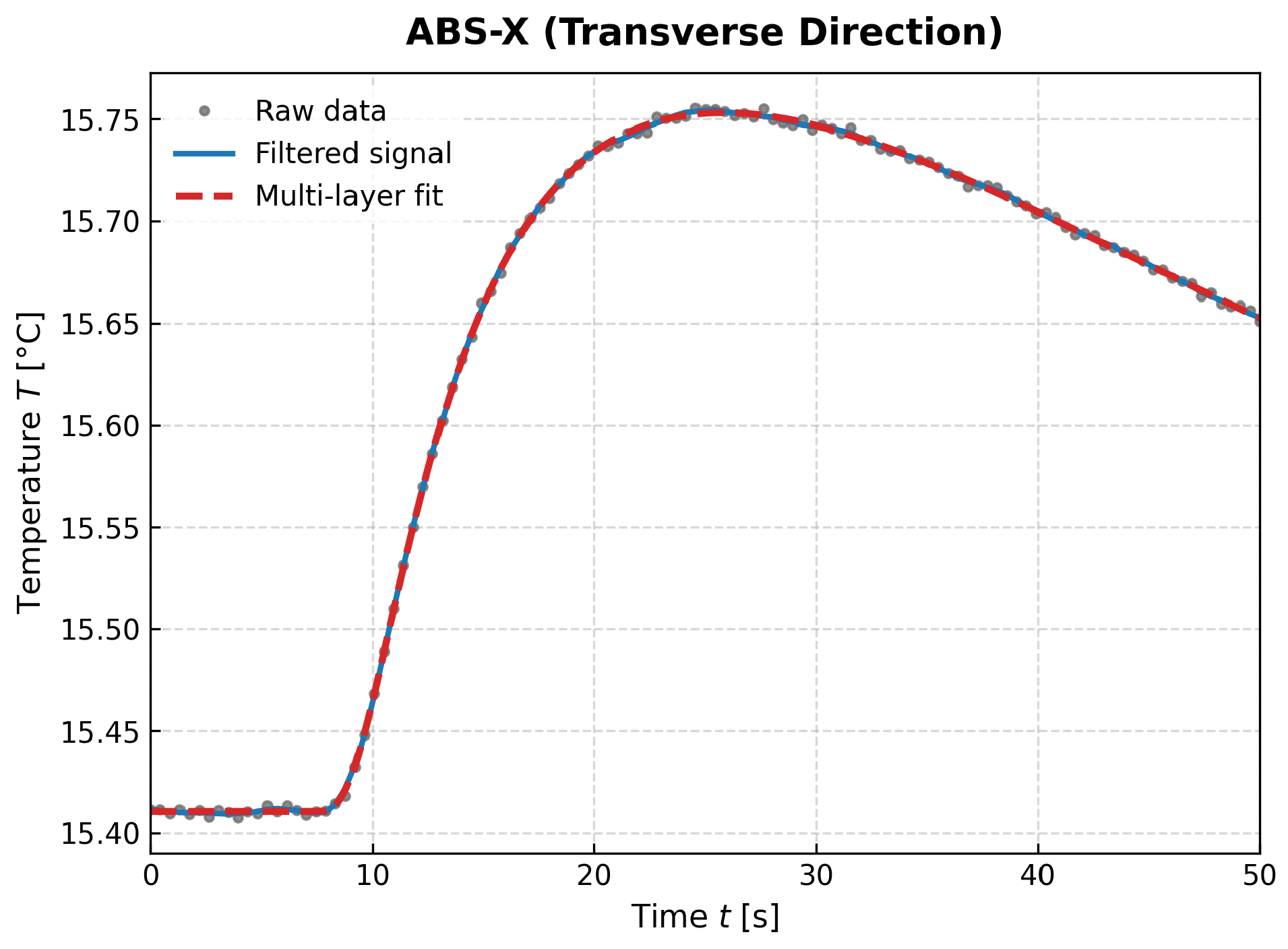
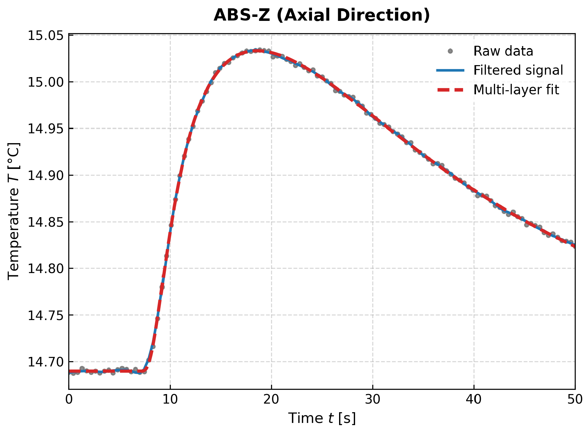
The transient temperature rise curves and non-linear model fits for ABS-X and ABS-Z are shown in Figure 4 and Figure 5, respectively.
For ABS-X (transverse direction), the temperature rise is highly attenuated and dispersed. The peak temperature rise of approximately 0.34 °C is reached at 25.8 s (19.3 s after the pulse), and the transient response shows a clear decay back to the baseline within the 50 s window. The fitted diffusivity is 0.4995 × 10 7 m2/s, corresponding to a transverse thermal conductivity of 0.1039 W/(m·K).
For ABS-Z (axial direction), the heat propagates faster. The temperature rise begins earlier, reaching a higher peak of approximately 0.34 °C at 18.6 s (12.1 s after the pulse). The fitted diffusivity is 0.8000 × 10 7 m2/s, which yields an axial thermal conductivity of 0.1664 W/(m·K). The anisotropy ratio A = λ z / λ x is calculated to be 1.60, confirming the significant influence of the printing direction on thermal transport.
These estimated thermal conductivity values show very good agreement with the anisotropic ranges reported in the literature for neat FDM-printed ABS. Specifically, Prajapati et al. [11] reported that the interlayer thermal contact resistance at the print boundaries significantly reduces through-plane (transverse) thermal conductivity, yielding values down to approximately 0.10 0.12 W/(m·K), depending on the internal void fraction. Conversely, in-plane (axial) conductivity values aligned with the filament deposition direction are typically reported in the range of 0.15 0.20 W/(m·K) due to the continuous polymer strand pathways and lower inter-filament thermal barriers [11]. The obtained transverse conductivity of 0.1039 W/(m·K) and axial conductivity of 0.1664 W/(m·K) fall squarely within these typical FDM ABS literature bands, validating the ability of our transient method to resolve build-induced anisotropy in additive manufacturing. Although the directional study here employs a single FDM polymer, the general applicability of the method is supported by three independent observations: the thickness-independent recovery of the isotropic reference standard across 1.0 3.0 mm (demonstrated in the reference standard validation above), the broad operating window mapped in Section 4.4 ( a 0.3 3 × 10 7 m2/s, λ 0.06 0.6 W/(m·K), spanning the range of common thermal polymers), and the agreement of the recovered ABS conductivities with independently published FDM-ABS values noted above.

4.3. Numerical Verification of the One-Dimensional Approximation

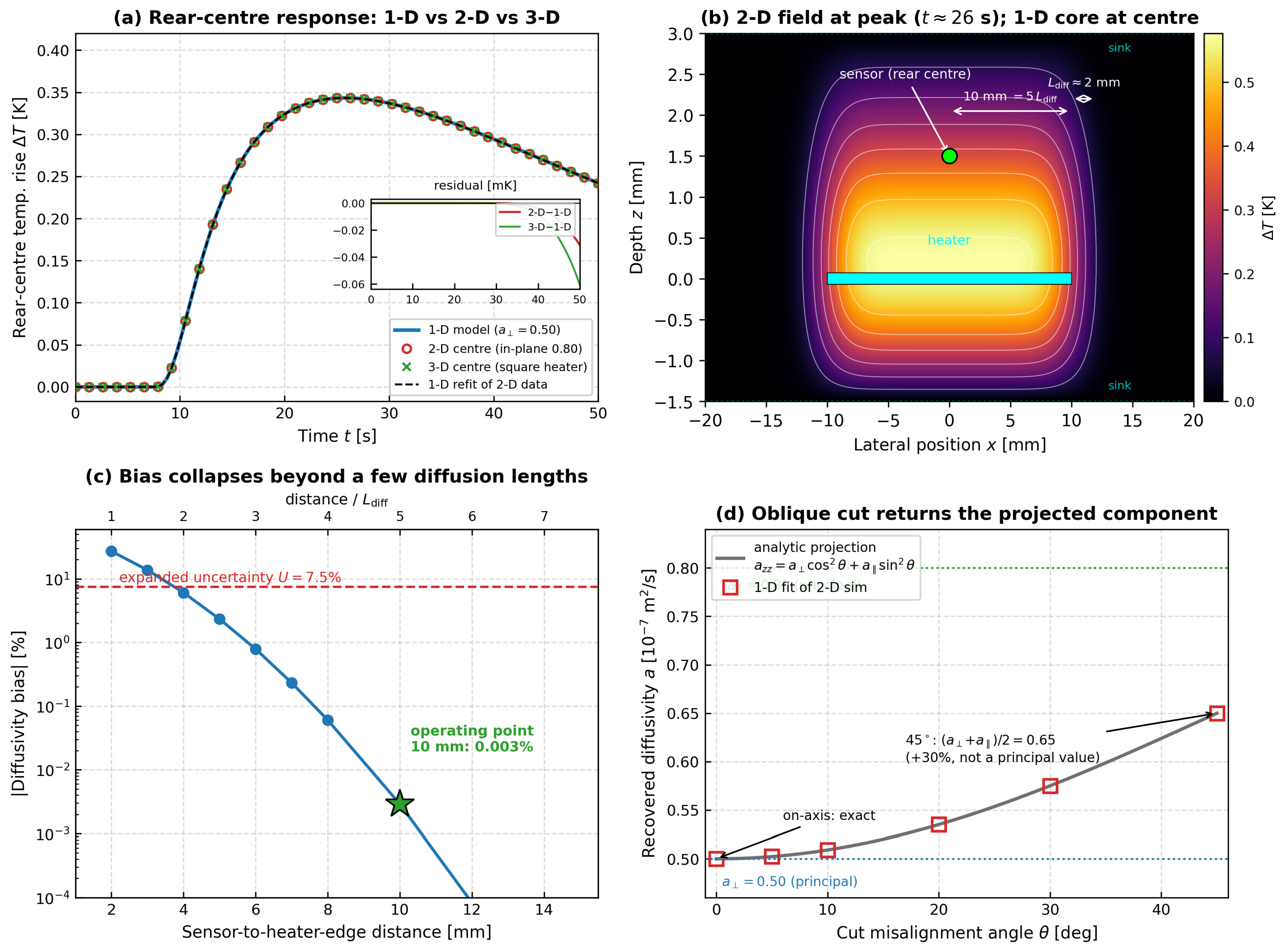
Because the printed ABS exhibits an in-plane diffusivity that exceeds the through-thickness value by 60 % (the axial-to-transverse ratio of 1.60 ), it is essential to confirm that lateral heat spreading does not bias the recovered through-thickness diffusivity, and that the one-dimensional reduction of Section 2.1 is quantitatively justified. The analytical diffusion-length argument ( L diff a t max 2.0 mm, against a 10 mm sensor-to-heater-edge distance) suggests the effect is negligible; this is verified directly with a forward two- and three-dimensional anisotropic simulation of the exact experimental geometry.
The full anisotropic heat conduction equation,
ρ c T t = λ x x 2 T x 2 + 2 λ x z 2 T x z + λ z z 2 T z 2 ,
was solved on the same asymmetric three-layer sandwich using a Crank–Nicolson finite difference scheme with an identical through-thickness discretization ( Δ z = d / 60 ), time step ( Δ t = 0.02 s), heater-source treatment, and isothermal-sink boundary conditions as the production one-dimensional estimator; the only physics added is the lateral (x) dimension, namely, the finite 20 mm heater embedded in the 40 mm specimen with adiabatic specimen edges. As a correctness check, the solver reproduces the one-dimensional response at the central sensor to machine precision (< 10 12 K) in the wide-heater limit (no lateral source edge), which guarantees that any departure observed for the finite heater originates solely from lateral conduction. To bound the genuinely three-dimensional spreading produced by the square heater, an analogous 3D run was performed in which the higher in-plane diffusivity ( 0.80 × 10 7 m2/s) was assigned to both in-plane directions, representing the absolute worst case for lateral heat loss.
For the worst-case transverse specimen (through-thickness a = 0.50 × 10 7 m2/s, in-plane a = 0.80 × 10 7 m2/s), the rear-center temperature history extracted from the two-dimensional field is visually indistinguishable from the one-dimensional model (Figure 6a; the residual remains below 0.05 mK throughout). Fitting this simulated two-dimensional signal with the production one-dimensional estimator recovers a = 0.50001 × 10 7 m2/s, a bias of only + 0.003 % ; the full three-dimensional worst-case run yields + 0.006 % (Table 3). Both values are more than three orders of magnitude smaller than the expanded measurement uncertainty of 7.5 % ( k = 2 ), confirming that the central sensor lies deep within the one-dimensional core of the temperature field (Figure 6b). This small bias is not an artifact of suppressed lateral physics: progressively narrowing the heater drives the bias upward in a controlled manner (to + 2.3 % when the sensor is 5 mm from the heater edge, and to + 27 % at a 2 mm gap, i.e., one diffusion length), and it falls below 0.01 % once the sensor-to-edge distance exceeds about four diffusion lengths (Figure 6c). The present apparatus operates at five diffusion lengths, placing it firmly in the negligible-bias regime.
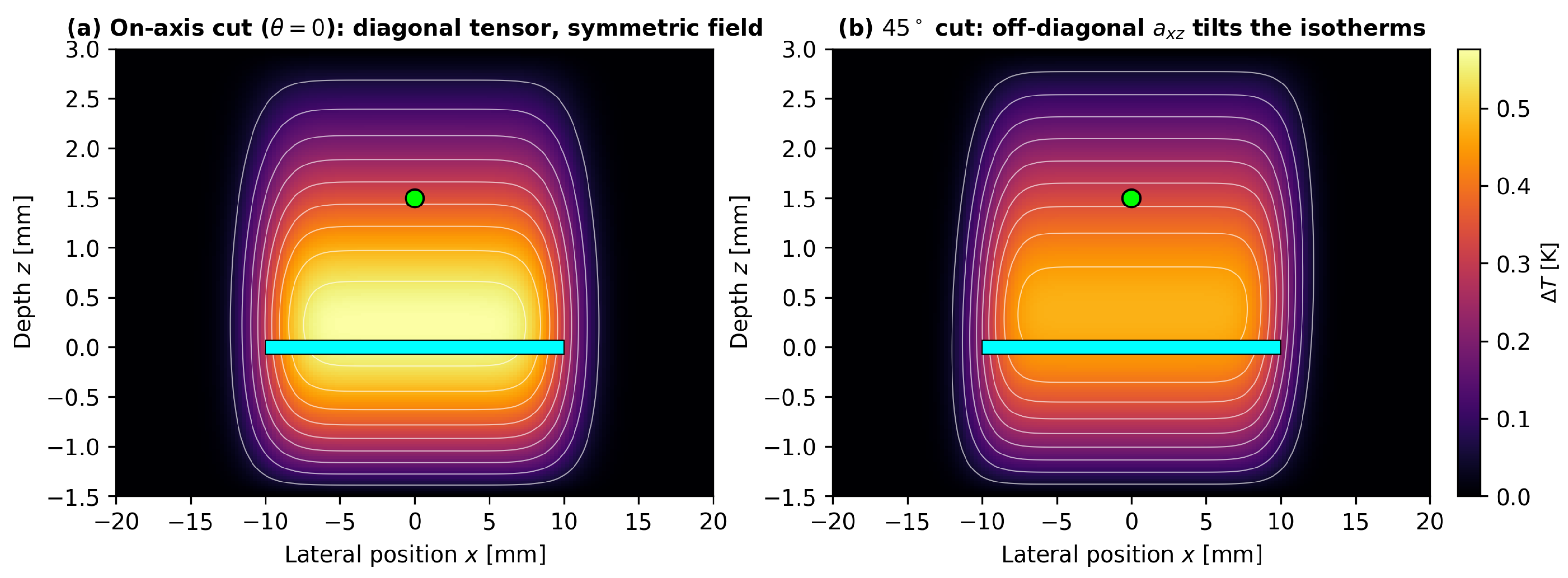
The behavior of an obliquely cut specimen further clarifies why principal-axis alignment is required. The present method resolves the principal-axis diffusivities by sequential, axis-aligned measurements; it does not diagonalize a full conductivity tensor from a single measurement. Cutting a specimen off-axis therefore violates the diagonal-tensor premise of Equation (1). To quantify this, the diffusivity tensor was rotated by an angle θ , and the two-dimensional simulation and one-dimensional fit were repeated. For a 45° cut (a fully non-diagonal tensor with a x x = a z z = 0.65 × 10 7 and a x z = 0.15 × 10 7 m2/s, principal values 0.50 and 0.80 ), the estimator returns a = 0.65000 × 10 7 m2/s, i.e., the diagonal through-plane component a z z = ( a + a ) / 2 and not a principal value; the off-diagonal coupling visibly tilts the isotherms (Figure 7) yet leaves the recovered diagonal component uncorrupted at the center. Across all angles the recovered diffusivity follows the analytic projection a z z ( θ ) = a cos 2 θ + a sin 2 θ to within 0.003 % (Figure 6d). Two conclusions follow. First, an oblique cut yields the geometrically projected axial component rather than a principal diffusivity, which is why principal-axis alignment is required. Second, the small-angle slope of this projection independently reproduces the cutting alignment contribution in the uncertainty budget (Table 1): the simulation gives a + 0.46 % diffusivity deviation at a 5° misalignment, in agreement with the tabulated 0.5 % .

4.4. Method Robustness and Operating Range

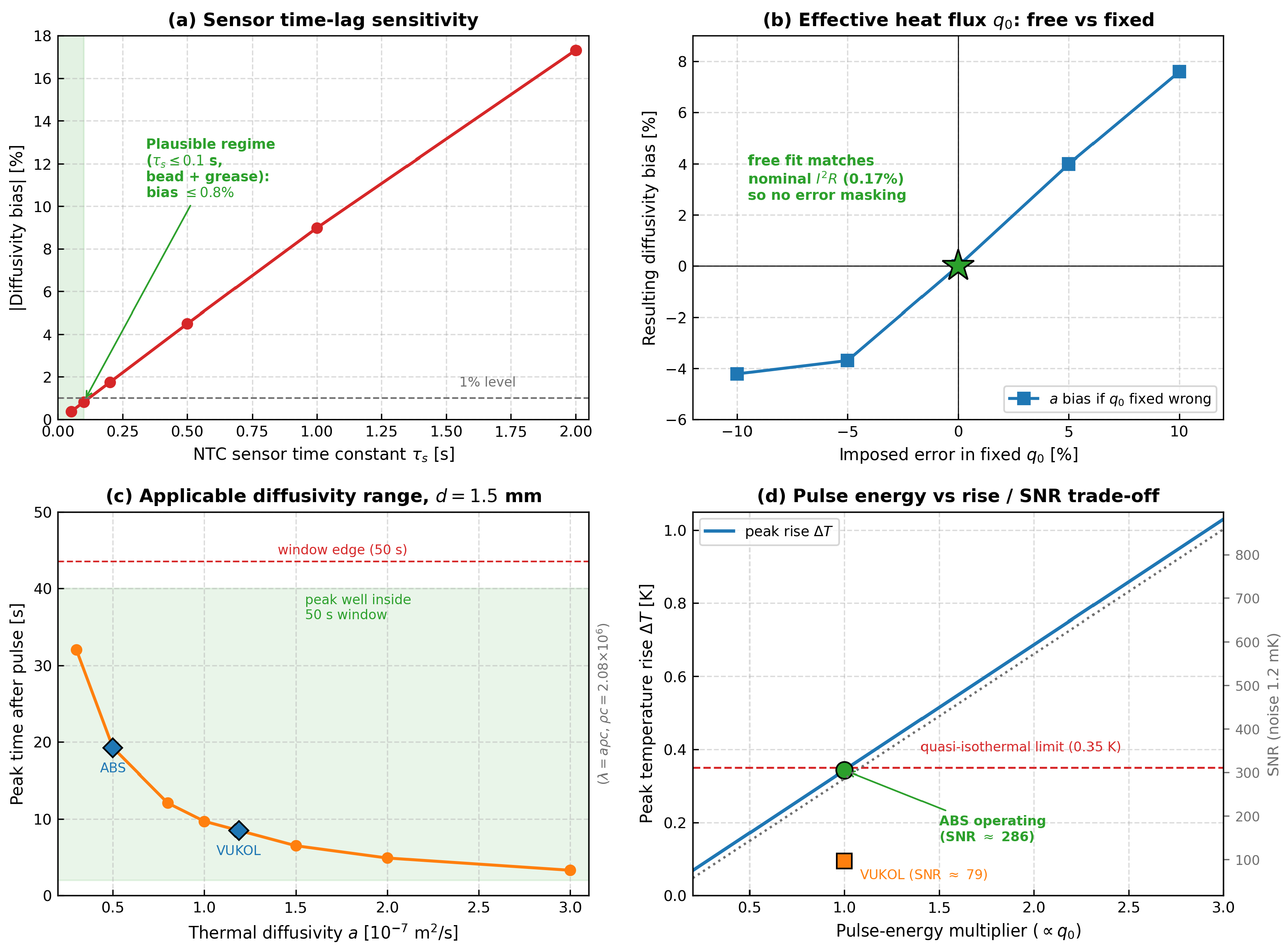
Beyond the dimensionality of the heat flow, several non-idealities of the physical measurement were examined quantitatively, each by applying the corresponding effect to the measured rear-side signal and re-estimating with the production solver. The results are summarized in Figure 8.
Sensor thermal response. An NTC thermistor has a finite heat capacity and contact conductance, so it reports the interface temperature with a first-order lag of time constant τ s . Applying such a first-order response to the measured rear-side signal and refitting with the lag-blind model produces a systematic under-estimate of the diffusivity that grows essentially linearly with τ s , at approximately 9 % per second (Figure 8a). For the bead thermistors used here, mounted in a micro-groove with thermal grease and clamped in intimate contact between solid polymer layers, the effective time constant is small (of the order of 0.1 s or less, far below the free-air value), so the associated bias is ≤0.8%. Two factors keep this contribution modest: the rear-side transient is slow (the peak occurs about 12 to 32 s after the pulse), so the relative lag τ s / t peak is small; and the same sensor measures the isotropic reference standard, against which the system is benchmarked. A sensor-response term is included in the uncertainty budget (Section 5). It should be noted that τ s cannot be identified from the in situ measurement itself: because the rear-side transient is slow, a finite sensor lag and a small change in diffusivity produce almost the same distortion of the recorded curve, so the two-parameter fit cannot separate them. The time constant is therefore not treated as a free parameter; it is characterized separately by an ex situ step-response test on the bare sensor, and its in situ influence is bounded by that independent value together with the agreement against the reference standard.
Effective heat flux: free versus fixed. Allowing the effective flux q 0 to float could, in principle, mask systematic model errors, but this is not the case here. When q 0 is left free, the fitted value agrees with the independently known electrical input ( I 2 R ) to within 0.17 % (Table 2: 22,662 versus 22,700 W/m2), so it recovers the physical flux rather than compensating for hidden errors; refitting with q 0 held fixed at that value returns an identical diffusivity, confirming that a and q 0 are independently identifiable (they imprint distinct, separable signatures on the transient, Figure 2a). Conversely, fixing q 0 at an incorrect value injects bias directly into a: a ± 5 % error in an imposed flux propagates to a 4 % error in the recovered diffusivity (Figure 8b). Because the true flux entering the specimen is not known a priori to better than a few percent from I 2 R alone (some Joule heat is stored in the foil heater and its leads and is lost to the front-side fixture rather than conducted into the specimen), estimating the effective q 0 is the more robust choice.
Filtering bias. The Savitzky–Golay pre-filter was checked for systematic bias by comparing the fits obtained with and without it: the recovered diffusivity changes by less than 0.05 % , and the run-to-run scatter of the estimate is essentially identical in both cases (about 0.11 % ), because the full-curve least-squares fit already averages the noise. The filter therefore serves visualization and peak identification without distorting the metrology.
Applicable range and pulse energy. The window of measurable properties is set by the requirement that the dispersed rear-side peak falls within the acquisition window. For the 1.5 mm configuration and the 50 s window, diffusivities from 0.3 to 3 × 10 7 m2/s (corresponding to conductivities of roughly 0.06 to 0.6 W/(m·K) at the present ρ c ) place the peak comfortably inside the record (Figure 8c); lower diffusivities require a thinner specimen or a longer window, since the characteristic time scales as d 2 / a . This scaling is precisely why the slower ABS specimens were measured at 1.5 mm and the faster isotropic standard at 3.0 mm. Regarding excitation energy (Figure 8d), the peak temperature rise scales linearly with q 0 ; the pulse is deliberately kept small to maintain the quasi-isothermal condition ( Δ T < 0.35 K), which preserves temperature-independent properties. Even so, the signal-to-noise ratio is ample (approximately 290 for the ABS specimens and approximately 80 for the lower-rise reference standard, with ambient baseline noise below 1.2 mK; Section 3.1), so that random noise contributes only about 0.1 % to the diffusivity estimate. Increasing the flux would raise the SNR further but would forfeit the quasi-isothermal advantage; the present operating point is a deliberate trade-off.

5. Uncertainty Analysis

A rigorous metrological evaluation was performed to compile the uncertainty budget according to the Guide to the Expression of Uncertainty in Measurement. This GUM framework has been widely applied to quantify the uncertainty propagation in advanced thermal characterization techniques, such as scanning thermal microscopy. Similar metrological evaluations have been implemented for standard heat flow meter systems to establish reliable uncertainty budgets for insulating materials. The combined standard uncertainty u c ( a ) is calculated by combining Type A and Type B contributions:
u c ( a ) = a x i u ( x i ) 2 .
The uncertainty budget is presented in Table 1.
The largest contributor to the uncertainty in thermal diffusivity is the specimen thickness d. Since the estimated diffusivity scales with the square of thickness in the solver ( a d 2 ), any geometric error is doubled in the final result. The specimen cutting alignment contribution accounts for the angular error when cutting the sample relative to the principal printing axes, which mixes the diagonal tensor components; this 0.5 % value is independently corroborated by the off-axis simulation of Section 4.3 (Figure 6d), which yields a + 0.46 % diffusivity deviation at a 5° misalignment. The sensitivity coefficients a / x i listed in Table 1 were determined numerically by introducing small perturbations to each individual input parameter x i in the non-linear multi-layer solver and computing the corresponding change in the estimated thermal diffusivity. Because the volumetric heat capacity ( ρ c ) is held constant during the optimization, the uncertainties in density u ( ρ ) and specific heat capacity u ( c ) do not influence the estimation of thermal diffusivity a, but propagate directly and linearly into the calculated thermal conductivity λ since λ = a ρ c . Consistent with the independent TPS determination of the reference standard’s volumetric heat capacity (which differs from the literature value by 3.8 % ), the specific heat uncertainty is assigned a conservative 3.7 % (density 1.0 % ), so that the conductivity budget reflects the measured volumetric-heat-capacity spread. The budget also includes the finite sensor thermal response, pulse-current and effective-flux stability, MOSFET pulse gating, specimen pore-distribution homogeneity, and the Savitzky–Golay filtering bias (quantified at < 0.01 % in Section 4.4). Each of these contributes ≤0.5% and, combined in quadrature, leaves the budget dominated by the specimen-thickness term, so the expanded uncertainty is essentially unchanged. The combined expanded uncertainty ( k = 2 ) is 7.5% for thermal diffusivity and 10.7% for thermal conductivity. The diffusivity uncertainty lies fully within the 5–10% range of high-end commercial systems for anisotropic materials; the larger conductivity figure is dominated by the conservatively assigned volumetric-heat-capacity term and would fall to ≈8% if the specific heat of the printed polymer were determined calorimetrically (DSC). This enlarged conductivity uncertainty does not affect the primary measurand, the thermal diffusivity, which is obtained independently of the volumetric heat capacity.

6. Conclusions

We have developed, validated, and metrologically characterized a transient thermal method utilizing a short rectangular current pulse excitation to determine the directional thermal properties of thin anisotropic polymer slabs. While the short-pulse transient principle and Crank–Nicolson inverse conduction are themselves established techniques, the contribution of this work lies in their integration into an accessible directional-characterization workflow: a custom, low-cost hardware architecture (an Arduino microcontroller and a constant-current MOSFET driver) is combined with an asymmetric multi-layer heat conduction model that explicitly accounts for boundary losses to the clamping system, removing the semi-infinite/adiabatic assumptions that fail on thin specimens. Directional properties are obtained from sequential, axis-aligned (unidirectional) measurements rather than from a single tensor inversion. By employing an ultra-low-energy excitation (0.2 s pulse, < 0.35 °C temperature rise), the polymer is maintained in a quasi-isothermal state, preventing temperature-induced physical changes. Because thermal diffusivity and conductivity are not independent ( λ = a ρ c ), the inverse problem is posed in terms of the diffusivity alone, with the volumetric heat capacity predetermined and fixed; this removes the ill-conditioning of a free two-property fit and yields a stable estimation solved via the implicit Crank–Nicolson method.
The method was validated using a VUKOL N22 potting compound as an isotropic reference standard and was subsequently applied to anisotropic 3D-printed ABS. The axial thermal conductivity of ABS was determined to be 0.1664 W/(m·K), compared to a transverse conductivity of 0.1039 W/(m·K), yielding a significant anisotropy ratio of 1.60. The one-dimensional reduction underlying the method was verified by direct two- and three-dimensional anisotropic simulations of the exact geometry, which bound the lateral-spreading bias below 0.01 % , even for the worst-case (highest in-plane diffusivity) specimen, and showed that an obliquely cut specimen returns the geometrically projected diagonal component rather than a principal value, confirming that principal-axis alignment is required by design. The robustness of the estimation to sensor thermal response, signal filtering, and effective-flux determination was quantified, and the applicable diffusivity range was mapped. The expanded metrological uncertainty is 7.5% for thermal diffusivity and 10.7% for thermal conductivity, the latter limited by the conservatively assigned volumetric-heat-capacity term and reducible by a direct calorimetric measurement of the specific heat. These results demonstrate the feasibility of using low-cost hardware combined with multi-layer boundary conduction modeling for the highly accurate, non-destructive directional characterization of highly dispersing anisotropic media. The present validation rests on an isotropic reference standard (measured at several thicknesses) and one anisotropic FDM polymer; the mapped applicable range ( a 0.3 to 3 × 10 7 m2/s, λ 0.06 to 0.6 W/(m·K)) indicates that the method extends naturally to other thin polymers and build orientations, and a broader inter-material and inter-laboratory study, together with direct calorimetric determination of the printed-polymer heat capacity, is a clear direction for future work.

Author Contributions

Conceptualization, M.J.; methodology, M.J.; software, M.J.; validation, M.J. and Š.H.; formal analysis, M.J.; investigation, Š.H.; writing (original draft preparation), M.J.; writing (review and editing), M.J. and Š.H.; visualization, Š.H. All authors have read and agreed to the published version of the manuscript.

Funding

This research received no external funding.

Institutional Review Board Statement

Not applicable.

Informed Consent Statement

Not applicable.

Data Availability Statement

The data presented in this study are available upon request from the corresponding author.

Conflicts of Interest

The authors declare no conflicts of interest.

Abbreviations

The following abbreviations are used in this manuscript:
ABSAcrylonitrile Butadiene Styrene
ADCAnalog-to-Digital Converter
CNCrank–Nicolson
DAQData Acquisition
FDMFused Deposition Modeling
GUMGuide to the Expression of Uncertainty in Measurement
NTCNegative Temperature Coefficient
VUKOL N22Polyurethane potting compound manufactured by VUKI a.s.
SNRSignal-to-Noise Ratio

References

  1. Stefanović, I.S.; Džunuzović, J.V.; Džunuzović, E.S.; Stevanović, S.; Dapčević, A.; Savić, S.I.; Lama, G.C. The impact of the polycaprolactone content on the properties of polyurethane networks. Mater. Today Commun. 2023, 35, 105721. [Google Scholar] [CrossRef]
  2. Džunuzović, J.V.; Stefanović, I.S.; Džunuzović, E.S.; Kovač, T.S.; Malenov, D.P.; Basagni, A.; Marega, C. Fabrication of polycaprolactone-based polyurethanes with enhanced thermal stability. Polymers 2024, 16, 1812. [Google Scholar] [CrossRef] [PubMed]
  3. Hardoň, Š.; Kúdelčík, J.; Janek, M.; Baran, A.; Kozáková, A.; Dérer, T. Halloysite nanotube enhanced polyurethane nanocomposites. Nanotechnol. Rev. 2025, 14, 20250248. [Google Scholar] [CrossRef]
  4. Cimbala, R.; Havran, P.; Király, J.; Rajňák, M.; Kurimský, J.; Šarpataky, M.; Dolník, B.; Paulovičová, K. Dielectric response of a hybrid nanofluid containing fullerene C60 and iron oxide nanoparticles. J. Mol. Liq. 2022, 359, 119338. [Google Scholar] [CrossRef]
  5. Havran, P.; Cimbala, R.; Dolník, B.; Rajňák, M.; Štefko, R.; Király, J.; Kurimský, J.; Paulovičová, K. Dielectric relaxation spectroscopy of hybrid insulating nanofluids in time, distribution, and frequency domain. J. Mol. Liq. 2024, 409, 125409. [Google Scholar] [CrossRef]
  6. Zohdi, N.; Yang, C. Material anisotropy in additively manufactured polymers and polymer composites: A review. Polymers 2021, 13, 3368. [Google Scholar] [CrossRef] [PubMed]
  7. Elkholy, A.; Rouby, M.; Kempers, R. Characterization of the anisotropic thermal conductivity of additively manufactured components by fused filament fabrication. Prog. Addit. Manuf. 2019, 4, 497–515. [Google Scholar] [CrossRef]
  8. Smirnov, A.; Solis Pinargote, N.W.; Khmyrov, R.; Babushkin, N.; Gridnev, M.; Kuznetsova, E.; Gusarov, A. Structure formation and thermal conduction in polymer-based composites obtained by fused filament fabrication. Int. J. Adv. Manuf. Technol. 2023, 129, 2677–2690. [Google Scholar] [CrossRef]
  9. Zohdi, N.; Nguyen, P.Q.K.; Yang, R. Evaluation on material anisotropy of acrylonitrile butadiene styrene printed via fused deposition modelling. Appl. Sci. 2024, 14, 1870. [Google Scholar] [CrossRef]
  10. Guo, H.; Niu, H.; Zhao, H.; Kang, L.; Ren, Y.; Lv, R.; Ren, L.; Maqbool, M.; Bashir, A.; Bai, S. Highly anisotropic thermal conductivity of three-dimensional printed boron nitride-filled thermoplastic polyurethane composites: Effects of size, orientation, viscosity, and voids. ACS Appl. Mater. Interfaces 2022, 14, 14568–14578. [Google Scholar] [CrossRef] [PubMed]
  11. Prajapati, H.; Ravoori, D.; Woods, R.L.; Jain, A. Measurement of anisotropic thermal conductivity and inter-layer thermal contact resistance in polymer fused deposition modeling (FDM). Addit. Manuf. 2018, 21, 84–90. [Google Scholar] [CrossRef]
  12. D’Amico, T.; Peterson, A.M. Bead parameterization of desktop and room-scale material extrusion additive manufacturing: How print speed and thermal properties affect heat transfer. Addit. Manuf. 2020, 34, 101239. [Google Scholar] [CrossRef]
  13. Selvamani, S.K.; Samykano, M.; Subramaniam, S.R.; Ngui, W.K.; Kadirgama, K.; Kanagaraj, G.; Idris, M.S. 3D printing: Overview of ABS evolvement. AIP Conf. Proc. 2019, 2059, 020041. [Google Scholar] [CrossRef]
  14. Le, T.-H.; Le, V.-S.; Dang, Q.-K.; Nguyen, M.-T.; Le, T.-K.; Bui, N.-T. Microstructure evaluation and thermal–mechanical properties of ABS matrix composite filament reinforced with multi-walled carbon nanotubes by a single screw extruder for FDM 3D printing. Appl. Sci. 2021, 11, 8798. [Google Scholar] [CrossRef]
  15. Rodriguez, A.; Fuertes, J.P.; Oval, A.; Perez-Artieda, G. Experimental measurement of the thermal conductivity of fused deposition modeling materials with a DTC-25 conductivity meter. Materials 2023, 16, 7384. [Google Scholar] [CrossRef] [PubMed]
  16. Trhlíková, L.; Zmeskal, O.; Psencik, P.; Florian, P. Study of the thermal properties of filaments for 3D printing. AIP Conf. Proc. 2016, 1752, 040027. [Google Scholar] [CrossRef]
  17. Bury, P.; Hockicko, P.; Jamnický, M. Transport and relaxation study of ionic phosphate glasses. Adv. Mater. Res. 2008, 39–40, 111–118. [Google Scholar] [CrossRef]
  18. Hockicko, P.; Bury, P.; Muñoz, F. Investigation of relaxation and transport processes in LiPO(N) glasses. J. Non-Cryst. Solids 2013, 363, 140–146. [Google Scholar] [CrossRef]
  19. Parker, W.J.; Jenkins, R.J.; Butler, C.P.; Abbott, G.L. Flash method of determining thermal diffusivity, heat capacity, and thermal conductivity. J. Appl. Phys. 1961, 32, 1679–1684. [Google Scholar] [CrossRef]
  20. Gustafsson, S.E. Transient plane source techniques for thermal conductivity and thermal diffusivity measurements of solid materials. Rev. Sci. Instrum. 1991, 62, 797–804. [Google Scholar] [CrossRef]
  21. Healy, J.J.; de Groot, J.J.; Kestin, J. The theory of the transient hot-wire method for measuring thermal conductivity. Physica B+C 1976, 82, 392–408. [Google Scholar] [CrossRef]
  22. Log, T.; Gustafsson, S.E. Transient plane source (hot strip) technique for measuring thermal transport properties. Fire Mater. 1995, 19, 43–49. [Google Scholar] [CrossRef]
  23. Cahill, D.G. Thermal conductivity measurement from 30 to 750 K: The 3ω method. Rev. Sci. Instrum. 1990, 61, 802–808. [Google Scholar] [CrossRef]
  24. Mandelis, A. Photoacoustic and Thermal Wave Phenomena in Semiconductors; North-Holland: Amsterdam, The Netherlands, 1987. [Google Scholar]
  25. Cahill, D.G.; Ford, W.K.; Goodson, K.E.; Mahan, G.D.; Majumdar, A.; Maris, H.J.; Photiadis, J.I.; Schmidt, K.E. Nanoscale thermal transport. J. Appl. Phys. 2003, 93, 793–818. [Google Scholar] [CrossRef]
  26. Ukrainczyk, N. Thermal diffusivity estimation using numerical inverse solution for 1D heat conduction. Int. J. Heat Mass Transf. 2009, 52, 5675–5681. [Google Scholar] [CrossRef]
  27. Janek, M.; Kúdelčík, J.; Hardoň, Š.; Gutten, M. Novel, cost effective, and reliable method for thermal conductivity measurement. Sensors 2024, 24, 7269. [Google Scholar] [CrossRef] [PubMed]
  28. Gunya, A.; Kúdelčík, J.; Hardoň, Š.; Janek, M. Thermodielectric properties of polyurethane composites with aluminium nitride and wurtzite boron nitride microfillers: Analysis below and near percolation threshold. Sensors 2025, 25, 4055. [Google Scholar] [CrossRef] [PubMed]
  29. Sanchez Pinosa, O.; Venerus, D.C. Thermal conductivity of poly(lactic acid) in solid and molten states and its dependence on temperature and crystallinity. ACS Appl. Polym. Mater. 2025, 7, 16585–16590. [Google Scholar] [CrossRef]
  30. Crank, J.; Nicolson, P. A practical method for numerical evaluation of solutions of partial differential equations of the heat conduction type. Math. Proc. Camb. Philos. Soc. 1947, 43, 50–67. [Google Scholar] [CrossRef]
  31. Sadeghi, M.; Behnia, F.; Amiri, R. Window Selection of the Savitzky–Golay Filters for Signal Recovery From Noisy Measurements. IEEE Trans. Instrum. Meas. 2020, 69, 5418–5426. [Google Scholar] [CrossRef]
  32. Savitzky, A.; Golay, M.J.E. Smoothing and differentiation of data by simplified least squares procedures. Anal. Chem. 1964, 36, 1627–1639. [Google Scholar] [CrossRef]
  33. Gu, J.; Zhang, Q.; Dang, J.; Xie, C. Thermal conductivity epoxy resin composites filled with boron nitride. Polym. Adv. Technol. 2012, 23, 1025–1028. [Google Scholar] [CrossRef]
  34. Ujfalusi, Z.; Pentek, A.; Told, R.; Schiffer, A.; Nyitrai, M.; Maroti, P. Detailed thermal characterization of acrylonitrile butadiene styrene and polylactic acid based carbon composites used in additive manufacturing. Polymers 2020, 12, 2960. [Google Scholar] [CrossRef] [PubMed]
Figure 1. Schematic diagram of the custom-built experimental setup showing the sandwich assembly of the planar heater, specimen, temperature sensors, and the thermal buffer within the 3D-printed gripper.
Metrology 06 00048 g001
Figure 2. Sensitivity analysis of the parameter estimation process: (a) scaled sensitivity coefficients of the rear-side temperature rise with respect to thermal diffusivity ( a T a ) and effective heat flux ( q 0 T q 0 ) showing distinct transient profiles; (b) objective-function contour map S ( a , q 0 ) displaying a well-conditioned optimization valley around the optimum solution.
Metrology 06 00048 g002
Figure 3. Representative experimentally determined temperature rise profile and non-linear multi-layer model fit for the isotropic VUKOL N22 reference standard, showing the raw measurements, the Savitzky–Golay filtered data, and the fitted curve.
Metrology 06 00048 g003
Figure 4. Representative transient temperature rise profile and non-linear multi-layer model fit for the 3D-printed transverse ABS-X specimen (perpendicular to layer interfaces).
Metrology 06 00048 g004
Figure 5. Representative transient temperature rise profile and non-linear multi-layer model fit for the 3D-printed axial ABS-Z specimen (parallel to layer interfaces).
Metrology 06 00048 g005
Figure 6. Numerical verification of the one-dimensional approximation for the worst-case anisotropic specimen. (a) Rear-center temperature rise from the one-dimensional model, the two-dimensional and three-dimensional simulations, and the one-dimensional refit of the two-dimensional data; the curves coincide (inset: residuals in mK). (b) Two-dimensional temperature field at the rear-center peak, showing the heater footprint, the isothermal sinks, the central sensor, and the one-dimensional core that surrounds it. (c) Magnitude of the recovered-diffusivity bias as a function of the sensor-to-heater-edge distance; the bias collapses well below the expanded uncertainty once this distance exceeds a few lateral diffusion lengths L diff , with the experimental operating point (10 mm) marked. (d) Diffusivity recovered from an obliquely cut specimen versus misalignment angle θ ; the fitted values follow the analytic tensor projection a z z ( θ ) = a cos 2 θ + a sin 2 θ and never return a principal value for θ > 0 .
Metrology 06 00048 g006
Figure 7. Simulated two-dimensional temperature field at the rear-center peak for (a) an on-axis cut, where the diagonal tensor produces a field symmetric about the sensor axis, and (b) a 45° oblique cut, where the off-diagonal tensor component a x z tilts the isotherms. The central sensor (green) and the 20 mm heater (cyan) are indicated.
Metrology 06 00048 g007
Figure 8. Quantified robustness of the method to non-idealities. (a) Systematic diffusivity bias versus NTC sensor time constant τ s ; the shaded band marks the plausible grease-coupled regime ( τ s 0.1 s, bias 0.8 % ). (b) Diffusivity bias incurred by fixing the effective heat flux q 0 at an incorrect value; a free fit matches the nominal flux (star), so a floating q 0 does not mask an error. (c) Applicable diffusivity range for a 1.5 mm specimen and 50 s window, set by the requirement that the response peak lies inside the record. (d) Peak temperature rise and signal-to-noise ratio versus pulse energy, showing the deliberate quasi-isothermal operating point.
Metrology 06 00048 g008
Table 1. Detailed uncertainty budget for the determination of thermal diffusivity a and conductivity λ using the custom short-pulse transient method.
Uncertainty SourceTypeUncertainty ValueSensitivity (Diffusivity)Standard Uncertainty u ( x i )
Time synchronization ( t 0 )B0.005 s 3.5 × 10 7  m2/s20.8%
Specimen thickness (d)B0.05 mm 8.0 × 10 5  m/s3.4%
Thermistor calibration noiseB0.005 K 1.2 × 10 5  m2/(s·K)1.0%
Thermistor resolutionA0.002 K 4.8 × 10 6  m2/(s·K)0.4%
Specimen cutting alignmentB5.0° 2.5 × 10 9  m2/(s·rad)0.5%
Specific heat capacity (c)B3.7%n/a3.7% (on λ )
Fixed density ( ρ )B1.0%n/a1.0% (on λ )
Numerical discretization errorB0.1%n/a0.1%
Sensor thermal response ( τ s 0.1  s)B0.1 s 4.5 × 10 9  m2/s20.5%
Pulse-current/effective-flux stabilityB0.5%n/a0.23%
MOSFET pulse gating (duration/jitter)B1 msn/a0.09%
Specimen homogeneity (pore distribution)An/an/a0.5%
Savitzky–Golay filtering biasBn/an/a0.05%
Combined uncertainty ( k = 1 ) 3.8% (a)/5.4% ( λ )
Expanded uncertainty ( k = 2 , 95%) 7.5% (a)/10.7% ( λ )
Table 2. Parameter estimation results for reference standard (VUKOL N22) and directional ABS samples using the asymmetric multi-layer solver. Values in parentheses denote parameter estimation standard errors ( k = 1 ).
MaterialDirection/Typea [ 10 7  m2/s] q eff  [W/m2] λ  [W/(m·K)] r  [K]
VUKOL N22      Isotropic Reference      1.1903 (0.0016)10,635.5 (6.0)0.2106 (0.0003) 4.37 × 10 3
ABS-XTransverse (Layers)0.4995 (0.0003)22,661.9 (6.1)0.1039 (0.0001) 7.33 × 10 3
ABS-ZAxial (Layers)0.8000 (0.0006)22,719.5 (11.4)0.1664 (0.0001) 1.11 × 10 2
Table 3. Bias of the one-dimensional estimator applied to simulated two- and three-dimensional anisotropic data for the worst-case (transverse) ABS specimen. For every configuration the estimator recovers the diagonal through-plane tensor component a z z ( θ ) = a cos 2 θ + a sin 2 θ to within 0.01 % ; on-axis this component equals the transverse principal value, whereas an oblique cut returns its geometric projection. Diffusivities are in 10 7 m2/s.
ConfigurationDiagonal a zz Recovered aDev. from a zz Dev. from a
On-axis transverse, 2D (in-plane 0.80 )0.500000.50001 + 0.003 % + 0.003 %
On-axis transverse, 3D (square heater, worst case)0.500000.50003 + 0.006 % + 0.006 %
5° misaligned cut, 2D (full tensor)0.502280.50229 + 0.003 % + 0.46 %
45° oblique cut, 2D (full tensor)0.650000.65000 + 0.000 % + 30.0 %
Disclaimer/Publisher’s Note: The statements, opinions and data contained in all publications are solely those of the individual author(s) and contributor(s) and not of MDPI and/or the editor(s). MDPI and/or the editor(s) disclaim responsibility for any injury to people or property resulting from any ideas, methods, instructions or products referred to in the content.