Abstract
Conducting measurements is a daily and time-consuming process that is critical to the manufacturing industry. The most widespread way to carry out the measuring process is using a Coordinate Measuring Machine (CMM). In this paper, a methodology is presented to accelerate the measuring procedure by optimally programming a CMM. The proposed methodology utilizes the information from a computer-aided design (CAD) file and the capabilities of CMMs in order to optimize the measurement process. An improved artificial fish swarm algorithm was modified to meet the requirements of the measurement process and the capabilities of the CMMs. In addition, the ant colony optimization method is applied to extract the optimal sequence of measurements throughout the multiple areas on the component. The resulting optimal path also utilizes the free areas between the different manufactured features of the component. Finally, the resulting path is collision-free, ensuring the integrity and the safety of the CMM. The proposed methodology is verified through real-world experiments.
1. Introduction
The advancement and the increasing application of manufacturing technology have widely expanded the use of CMMs. Measuring the tolerances of manufactured parts is a required daily concern in the production cycle of the manufacturing industry. A key task of this process is the inspection of the manufactured part using a CAD drawing. Many of the manufactured parts come from the same CAD drawing. Thus, their inspection process can be automated and performed repeatedly by a CMM without the need for operator intervention. The CMM’s probe path planning can be generated either manually or using a path planning method. Several methodologies have been developed for finding the optimal path that connects two points without causing any collision or damage to the robot. Some of the successful path planning algorithms are the ant colony optimization (ACO) [1], genetic algorithms [2], rapidly exploring random tree (RRT) [3], neural network [4], probabilistic roadmap algorithm (PRM) [5] and A* algorithm [6].
Coordinate measurements can be performed using a CMM or directly on machine tools. Measuring systems can be classified into two main types based on whether they are equipped with contact or non-contact measuring probes [7]. The machines equipped with contact measuring probes are widely used in inspection tasks. However, the disadvantage of their inherent low speed is the only reason that prevents them from being used profitably for the repetitive measurement of complex parts [8]. During the measurement process using a CMM, only a finite number of points on the examined part are sampled [9].
A CMM is utilized to capture the spatial coordinates of a single or multiple points on the component’s surfaces. The acquired data are used to mathematically formulate the geometrical and dimensional attributes of the components. Parameters measurable with a CMM include distances between points, feature centers, lines or planes, as well as diameters of circular, cylindrical or spherical features, and angles formed between lines, planes or axes. Moreover, the evaluation of parameters related to the tolerances can be performed such as flatness, cylindricity, surface profile, parallelism, angularity, perpendicularity, coaxiality and symmetry. These parameters provide essential information for ensuring that the examined component complies with the design specifications.
1.1. Literature Review
Sadaoui et al. proposed an approach for generating the path of a laser sensor integrated with a CMM on different measurement planes [10]. Morozov et al. suggested a computer-aided scan path planning applied using a robotic arm for non-destructive testing [11]. Masood et al. nominated an algorithm to generate the tool path using point cloud data [12]. Fountas and Vaxevanidis used swarm-based evolutionary algorithms for the 3D tool path trajectory optimization [13]. Lin et al. recommended an approach for measurement path planning of airfoils [14]. Stojadinovic et al. presented a path planning model based on a CAD model for measuring a prismatic part using a CMM [15]. Wan et al. suggested an optimization to the inspection path of a propeller to reduce the inspection time by 60% and decrease the inspection error by 8 μm [16]. Ma et al. proposed a contour-based path planning method using Monte Carlo estimation in the cost function [17]. Mansour et al. proposed a hybrid optimization method to determine the optimal placement of a measured component in the operation space of a CMM and the optimal trajectory of the CMM’s probes in order to reduce the measurement time [18].
Jin et al. proposed a modified RRT algorithm for generating paths and used a B-spline interpolation algorithm to smooth them [19]. Ou et al. introduced a method that combines adaptive visibility graphs and the A* algorithm to improve the path planning efficiency of mobile robots [20]. Li et al. used an improved twin delayed deep deterministic policy gradient algorithm for improved path planning generation in a dynamic environment [21]. Shujuan et al. used an A*, the Hungarian and a genetic algorithm with an improved bat algorithm for assigning multiple target points and solving the path planning problem in a dynamic environment [22]. Huang et al. proposed an improved bidirectional RRT* path planning algorithm with adaptive search strategy assignment mechanism in order to find the optimal path in 3D environments [23]. Zhou et al. suggested a bio-inspired algorithm that uses the basic mechanisms of plant growth, including phototropism, negative geotropism and branching for finding the optimal path in a 3D environment with static obstacles [24]. Chowdhury et al. nominated a reverse glowworm swarm algorithm for solving the path planning problem in a 3D environment with static and dynamic obstacles [25].
1.2. Problem Statement
Many times, multiple measurements in different areas need to be taken to fully measure a component. Using a CMM with a contact measuring probe, due to its manufacturing limitations, requires more time, and the search for a solution to speed up the measuring process using the existing machines is an open field of research. The measuring time can be increased unnecessarily due to the fact that the measurements in the different areas of the part are not performed in the optimal order, and the measuring probe travels long distances from one area to another. Thus, the component’s measurement time is increased without gaining any advantage.
1.3. Contribution
Currently, despite the wide application of path planning algorithms in mobile robots, their use in measuring multiple path optimization is very limited. In this paper, the methodologies proposed in [26,27] are combined in order to minimize the probe’s travel distances between the multiple areas of measurements. Furthermore, a novel use of the grid environment for representing 3D CAD components in the context of path planning is presented. The objective function of [27] is also modified properly in order to enable the algorithm to be applied for the purpose of finding the optimal path in an environment where the number of obstacles is significantly higher than the number of free movement points. The methodologies were applied for the 3D path planning of CMM with a contact measuring probe for the task of inspection of manufactured parts from a CAD file in order to optimize a production cycle in the manufacturing industry. Through the presented methodology, a new field of application for the well-known Traveling Salesman Problem (TSP) is highlighted, extending its use beyond classical optimization contexts. Specifically, TSP principles are adapted and applied to optimize measurement sequencing in CMM processes, demonstrating their relevance in a novel industrial and metrological setting.
2. Materials and Methods
2.1. Three-Dimensional Grid Creation
The modeling of the CMM’s movement space around the measured component is accomplished using the 3D grid environment method. The 3D grid consists of many elementary finite rectangular parallelepipeds suitably arranged in the 3D space. The space occupied by each elementary finite rectangular parallelepiped is represented by a discrete point placed at the coordinates of its gravity center. Each discrete point is associated with the volume defined by the boundaries of its corresponding elementary finite rectangular parallelepiped. Every discrete point functions independently, without interdependence on neighboring points. The 3D grid environment is employed to computationally simulate the physical volume of a given area. Figure 1a shows the elementary finite rectangular parallelepiped and its discrete point in red. Figure 1b shows the 3D grid environment.
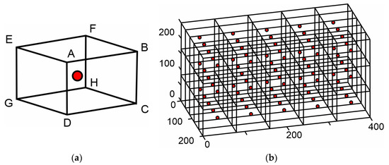
Figure 1.
Example of 3D grid environment creation: (a) elementary finite rectangular parallelepiped; (b) 3D grid environment example in mm.
Then, the component’s CAD is placed within the 3D grid and the discrete points of the elementary finite rectangular parallelepipeds whose areas intersect the CAD model are considered as obstacles and are represented in black. It is worth noting that even if a small part of the CAD is located in the region of the finite rectangular parallelepiped, its discrete point is considered an obstacle. Figure 2a shows a 2D example of placing a CAD file in a grid environment and Figure 2b the representation of obstacles. The modeling accuracy depends on the grid’s density.
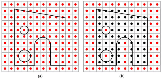
Figure 2.
Example of creation of the grid environment using the information from a CAD file: (a) incorporation of 2D CAD representation in grid environment; (b) depiction of a CAD surface within the grid environment by using obstacles.
Figure 3 shows an example of defining the dimensions of the grid environment for a 3D component. In this example, it is assumed that the measurements will be at the top area of the part. The dimensions are defined based on the areas of the piece where the measurements will be conducted. If measurements are to be taken on the sides of the piece, additional space needs to be set to examine alternative paths that better simulate the real-world movement environment of the CMM’s probe. However, defining too much extra space leads to an increase in the number of the grid environment’s points and requires more computational time to solve the problem without necessarily leading to improved solutions.
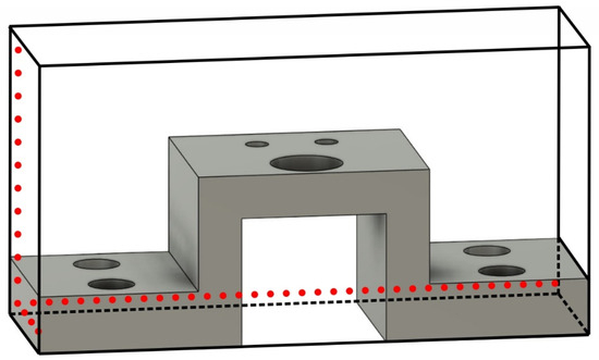
Figure 3.
Example of defining the dimensions of the 3D grid environment taking into account the component’s measurement areas.
2.2. CMM’s Movement Simulation
Simulating the CMM’s real-world motion capabilities in the artificial 3D environment is important for the results credibility. The CMM can move freely in all directions of the 3D space, into its workspace. The motion capabilities in all directions and the 3D model of 24 possible movement points described in [27] can perfectly simulate the movement capabilities of the CMM and were used in this paper. The artificial fish can move in all the environment’s discrete points except in those that are considered obstacles. The grid environment is defined within the CMM workspace; if any elementary finite rectangular parallelepiped is located beyond, the workspace’s spatial boundaries are identified as obstacles.
Some other advantageous factors during the CMM’s probe path planning process are the linear motion between the coordinates in 3D space and the small number of points on the final path. The measuring probe is very sensitive and if it unexpectedly touches a part of the component during its transfer from one area to another while the measuring process is not being performed, it may break or the probe protection system of the CMM may be activated and completely immobilize the machines. Both circumstances negatively affect the measuring process by greatly increasing the cost and the measurement time unnecessarily. The length of the curved movement between two points can, in some cases, be shorter than the combination of multiple linear movements in order to travel the same distance. This phenomenon occurs due to the discretization of the environment. However, during the transfer process, the probe is located at a greater distance from the examined part and the contact due to some micro-scaled mistake placement of the piece becomes more difficult. Figure 4 shows an example of transferring from one point to another using a curved trajectory and a multiple linear trajectory. The reduced number of points of the total path accommodates the rectilinear transport from one point to another without intervening intermediate points of the same line equation and the resolution of movement constraints in a grid environment as described in [28]. Moreover, the slightly enlarged representation of the CAD model in the form of obstacles described in Section 2.1 assists in avoiding this phenomenon.
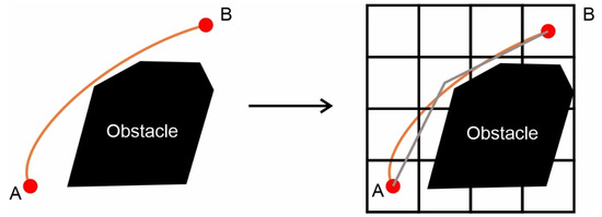
Figure 4.
Examples of curved and multi-linear paths to connect point A to point B.
The method of multiple lasers as described in [27] ensures the above-mentioned advantages and, as shown in [28], the formed path is expected to be shorter than the one formed in [26] and to simulate more accurately the real-world movement capabilities of CMMs. The difference in the length of the formed paths is mainly due to the fact that the methodology presented in [27] adopts the 3D model of 24 possible movements points, while the methodology in [26], the model of 8 possible movement points. An additional reason for the reduction in path length is the implementation of the ray tracing algorithm in [27], which further decreases the length of the formed paths.
2.3. Three-Dimensional Path Creation
Adopting the environment creation methodology described in Section 2.1, depending on the complexity of the component, dense and complex 3D environments are often created. The number of obstacles may exceed the number of feasible movement points. Therefore, the 3D path planning algorithm should be able to effectively respond to the characteristics and peculiarities of the environment.
The 3D path planning problem is solved using the improved artificial fish swarm algorithm (AFSA) and the multiple laser method proposed in [27]. The artificial fish swarm algorithm is a parallel stochastic search algorithm. Some of the beneficial features of the algorithm are the robustness, large tolerance of parameter setting, global searchability and the infectivity of initial values. Its main disadvantage in the process of finding the optimal path in 3D environment is the lack of some form of memory which is effectively solved by the multi-laser method. On the other hand, the ant colony optimization (ACO) proposed in [26] is extensively used to solve the path planning problem but is relatively sensitive to the initial parameters, which are greatly affected by the number, the location and the density of the obstacles in the 3D environment. In addition, the suboptimal parameter tuning can reduce the algorithm’s searchability. In a dense 3D environment, the ACO faces difficulty in finding the optimal path, requiring several iterations and increased computational time to find the optimal path.
General Algorithm’s Methodologies
The improved AFSA, which is used to find the optimal 3D path, includes the methodologies proposed in [27]. The utilized algorithm integrates the AFSA with the ray casting algorithm.
The CMM probe is capable of unrestricted movement in all directions of the 3D environment. The path planning algorithm needs to accurately simulate this capability. Thus, the 3D model of 24 possible movement points is used. The 24 possible movement points model allows the agents to select their next position from a set of 24 movement points in 16 different directions from their current position. The algorithm in [26] employs the model of 8 possible movement points. This model enables movement to the 8 closest points in 8 different directions from its current position. The 3D models of 8 and 24 possible movement points model allow the agent to additionally navigate to all vertical discrete points of the 8 or 24 fundamental possible movement points. Figure 5a and 5b show the 8 and 24 possible movement points models, respectively.
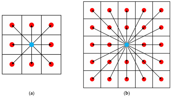
Figure 5.
Representation of movement points navigation models from the current position: (a) the navigation model of 8 possible movement points; (b) the navigation model of 24 possible movement points.
AFSA is a bio-inspired artificial intelligence algorithm that computationally simulates 4 behaviors of natural fish swarms in order to solve complex optimization problems [29,30]. Nominally, the behaviors employed are prey, follow, swarm and random behavior. Behaviors are used to select the agent’s next movement point from the set of points resulting from the 3D 24 possible movement points model.
In prey behavior, the artificial fish selects the next possible movement point from its visual field according to Equation (1). The indexes i and j indicate the current and the next possible location, respectively. The selection of the next possible point of movement is followed by the evaluation of the value of its objective function. A comparison is conducted between the values of the objective functions of the current position fi(x,y,z) and the selected one fj(x,y,z). If the value fj(x,y,z) > fi(x,y,z) the artificial fish will move a step closer to the selected location according to Equation (2). The Euclidean norm ||Xj − Xi|| = dij represents the distance between the points i and j. If this condition is not satisfied, the process of selecting the next movement point according to Equation (1) will be repeated. This procedure can be repeated as many times as specified by the parameter fishTryNum. If the number of attempts exceeds the number specified by the parameter fishTryNum, then the random behavior is performed.
The follow behavior compares the value of the objective function of the best possible position of the other fish in the visual range with the current position of the swarm. In the case where the value of the objective function of the current position is lower than the optimal one and the optimal position is not crowded, the artificial fish moves closer to the optimal position according to Equation (3). If any of the above conditions are not satisfied, the prey behavior is executed. Equation (4) determines whether the crowded condition is satisfied. The variable nf represents the number of fish in the location and N is the total number of previous fish. The variable δ represents the crowded degree 0 < δ < 1.
The swarm behavior compares the value of the objective function of the central position of the previous fish and the current. The center position is calculated according to Equation (5). The index C represents the center position. In the case where the value of the objective function of the central position is greater than the current one and is not crowded, then the artificial fish moves towards it according to Equation (6). The crowded degree is calculated according to Equation (4). In case the above conditions are not satisfied, the prey behavior is executed.
The random behavior moves the fish randomly to a new location according to Equation (7). The implementation utilizes the behavior proposed in [28] to replace random behavior.
The approaches provided in [27] regarding the 3D heatmap model, including both 3D simple and advanced eliminations, were also employed. The integration of the ray casting algorithm into the AFSA is accomplished as described in [27].
The objective function in Equation (8) was used to find the optimal path. In Equation (1) x, y, z are the Cartesian coordinates of the points, the index i represents the current location of the fish and the index ending represents the ending point location. The coefficients w1, w2 and w3 represent the importance of the safety value factor and the total movement point factor and the distance of the current fish position to the final position, respectively. Compared to [27], the coefficient w3 was added to improve the evaluation of each possible movement point due to the increased mesh density and the existence of multiple obstacles.
Equations (9) and (10) are utilized to calculate the safety value and total movement point factor, respectively. The variable k is the total number of discrete points that a fish can move from its current location, the variable g is the total number of points that are considered as obstacles from its current position and the variable w is the total number of eliminated points from the set of possible movement points due to the existence of obstacles.
2.4. Travel Salesman Problem
The optimal sequence of conducting the measurements in different areas of the component is found by solving the TSP. The TSP in a 3D environment with obstacles was solved according to the methodology proposed in [26]. First, a rectangular matrix A with dimensions m m is created. The number m is equal to the total number of different areas where the probe needs to be moved to take measurements. The rows of the table correspond to the starting measurement location of the path and the columns to the ending point. The elements of the table correspond to the length of the route formed for the corresponding pair of starting and ending points. In the elements of the main diagonal of the table, the starting and ending points coincide and the length of the route is 0. Completing all elements in the table is a fundamental requirement for solving the TSP. The length and the shape of the formed path were found according to Section 2.3 and inputted to the ACO for solving the TSP.
In addition, similar to matrix A, matrix B is created. The only difference between them is that instead of inputting the lengths of the paths, the value of the pheromone’s value is stored. The trajectory must be executed by the CMM’s probe in a continuous movement. Consequently, the ending point of a given path is automatically designated as the starting point of the subsequent path. In order to find the optimal solution, it is also required to define the starting location of the measurements. From the current position, the objective functions are calculated for all possible movement positions, and the roulette method is used to select the next location. The roulette method is a stochastic technique for conducting a selection among a set of choices with different possibilities of selection. The possibilities of selection of each point from the set kp of possible movement points are calculated based on Equation (11). The variable τ expresses the pheromone concentration for the given time t while fi,j(t) is the objective function. The variables α and β are the weighting factors of each term.
The selected point is recorded as the current position of the ant, and the process is repeated until the route formed has passed through all the desired points. When the process of selecting the next point of movement is complete and the ant is transported to it, the pheromone is locally updated in the corresponding element of table B according to Equation (12). The coefficient q denotes the rate of decrease in the pheromone q . The local pheromone update decreases the possibility of reselecting the same point from the next ant. This strategy encourages the artificial ants to explore different alternative paths throughout the environment. Once all ants in the colony have completed the path generation process for the shortest path in the colony, the global pheromone update is performed according to Equations (13) and (14). The coefficient p denotes the rate of update of the general pheromone. The increase encourages the ants of the next colony to explore solutions around an existing solution so as to correct possible errors. The coefficients gAnt and D are constants, Nmax denotes the maximum number of iterations, Nc the number of iterations performed and the denominator of Equation (14) denotes the length of the chosen path formed by the artificial ant kAnt. The solution of TSP requires the definition of some additional parameters: the parameter MaxItTSP, representing the maximum number of iterations, and initPher, denoting the initial pheromone value.
The objective function used for solving the TSP is given by Equation (15). It only takes into account the distance of the current point from the next possible point. The index cur denotes the current position and the index the next possible position.
2.5. Measurement Parameters Definition
The presented methodology facilitates the measurement of all parameters that can be evaluated by the CMM. As outlined in the introduction, the evaluation of geometrical characteristics is carried out by creating mathematical models of the component’s surfaces based on the coordinate information of the points collected by the CMM. These measurement operations can be classified into two categories, depending on whether they require the recording of a single point in a region or the acquisition of multiple points. Measurement parameters such as line creation or plane definition require the recording of a single point in an area, while parameters such as circle creation require the recording of multiple points. The objective of the proposed methodology is to determine the shortest possible path necessary to perform the predefined measurements. For parameters that require the acquisition of multiple points, the path length associated with their execution is predetermined and remains constant, regardless of the measurement sequence. For this reason, such parameters are represented in the grid environment by a point that may be positioned either at the beginning or within the central region of the measurement area. The placement of the points depends on the spatial extent of the region encompassing the acquired measurement data. In the case of circular features, for example, where a minimum of three closely positioned points is required to define the geometry, the representative point is typically located at the center of the circle. Similarly, parameters requiring the acquisition of a single point are also represented by a single point within the grid environment.
Figure 6 summarizes the execution sequence of the previous steps.
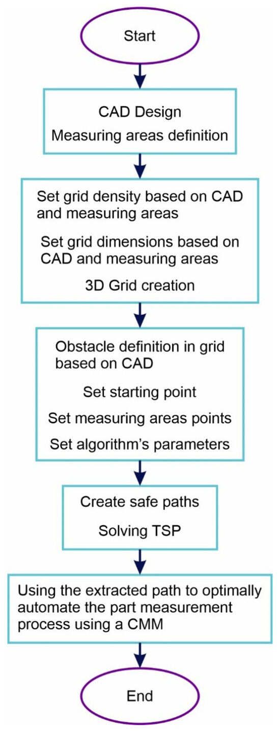
Figure 6.
Steps of the procedure.
3. Results
The 5-axis CMM shown in Figure 7a was used for the application of the proposed procedure. Figure 7b shows the experimental measuring component. A large number of measurement procedures provided by CMMs can be simulated on the experimental measuring component. More specifically in this example, measurements are conducted on the inner perimeter of two holes, around the small cylinder in area 1, at two points on the surface of the workpiece and on the inclined surface of area 8. In Figure 7b, the positions of the points on the surface of the component are shown in purple. Furthermore, in this example, a thin grid environment is used to emphasize the description and clear presentation of the methodology. The positions of the measurement points and the accuracy of the results can be significantly improved by using a denser grid environment. The presented methodology was developed using Matlab R2016a (The MathWorks, Inc., Natick, MA, USA) and python (Python Software Foundation, Wilmington, DE, USA). The operation of the CMM was facilitated using the PC-DMIS 2021.2 (Hexagon Manufacturing Intelligence, North Kingstown, RI, USA) software package.
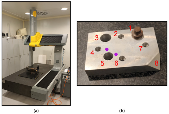
Figure 7.
Experimental set-up: (a) 5-axis Coordinate Measuring Machine (CMM); (b) experimental component.
Figure 8 shows the 3D environment and the modeling of the component in the form of obstacles resulting from the CAD file. The points where the measurement procedures will be performed are marked in green. In the case where the measurement points are located around the perimeter of the component, during the environment creation process, it would be necessary to have free movement points around the component. However, in the examined scenario, the measurement points are located on the component, thereby it is not necessary to add additional free movement points surrounding the component. Adding additional free points increases the complexity of the 3D space and the computational resources without benefiting the search for finding a shortest path.

Figure 8.
Three-dimensional representation of the measurement environment.
The parameters used for the 3D path planning algorithm are the following, MaxIt = 50, MaxStepsNum = 30, numFish = 130, fishTryNum = 15 and δ = 0.2, w1 = 1.4 w2 = 0.3, w3 = 4. The variable MaxIt represents the maximum iteration number for AFSA, MaxStepsNum specifies the maximum allowable number of nodes in a generated path; if the MaxStepsNum number is exceeding, the path is discarded as a non-optimal solution. The parameter numFish represents the number of fish in the swarm. Regarding the creation of the obstacle, heatmap were defined as obsHeatVal = 150, heatIncrCoef = 0.4, obsNearHeatVal = 90, obsNearHeatVal2 = 40. The parameter obsHeatVal represents the heat value of each obstacle, the heatIncrCoef corresponds to the coefficient of increasing the heat across the map, the parameters obsNearHeatVal and obsNearHeatVal2 represent the update of heat values in the first and the second stage of heatmap’s creation. The bonuses of the heatmap are divided in the following way. If the heatmap value, hv, for the point where the fish is located is less than , then the objective function of the possible points that are distanced is calculated by a coefficient bh = 1.15, where mh is the mean of heatmap values, da is the length of the side from an elementary square of the grid. If the and for the points distanced or da the bh = 1.06. If the and for the points distanced bh = 1.06. If for the points distanced or bh = 1.06. The parameters for ACO and solving the TSP are the following MaxItTSP = 40, α = 1, β = 1, q = 0.2, p = 0.3, gAnt = 0.2, D = 100 and initPher = 600. Comprehensive descriptions of the parameter tuning process in ACO and AFSA are available in the original research works cited in references [26] and [27], respectively.
In this section, the results from the proposed procedure are presented. Figure 9 shows in magenta the path resulting from the above procedure. The algorithm efficiently finds the shortest path that connects all the measuring points. Thus, the sequence of carrying out the measurements is determined in order to reduce as much as possible the probe’s transfer time between the measurement areas and accelerate the measuring process. It is worth noting that the final path even takes advantage of the size of the hole in area 3 so that the probe approaches the target point passing as close as possible to the component’s surface without touching it. The straight segments that connect the distant target points without passing through any intermediate point are due to the use of the multiple laser method.
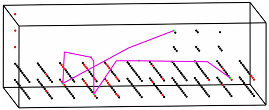
Figure 9.
Resulting path of measurements.
Figure 10a–h show the CMM’s probe location during the execution of the resulting path. The probe was successfully moved to the final coordinates of the resulting points without colliding with the experimental component. As can be seen from the images, the piece was placed in the inner part of a vice in order to immobilize it and keep it stationary during the measurement process. This procedure is widely applied in the measurements. It is worth noting that the positions of the vice and the point O (0,0,0) of the component’s virtual grid in the CMM operating space are known. The transfer of the probe to the initial coordinate position of the resulting path is carried out from a safe area to ensure that there will be no collision before the path is executed. As the measurements are to be performed above the plane of the vice and the designed path will lie within the component’s volume or the space above it, the vice does not influence the measurement process and therefore does not require to be modeled in the grid environment. If measurements were to be conducted on the side surface of the component, it is probable that the created path would traverse through the spatial area occupied by the vice. Under these circumstances, it would be necessary to model in the grid environment the parts of the vice that may hinder the movement of the probe. The entire vice would need to be modeled in the grid environment in the case where the locations of the examined measurements were on multiple components in the CMM’s operation environment.
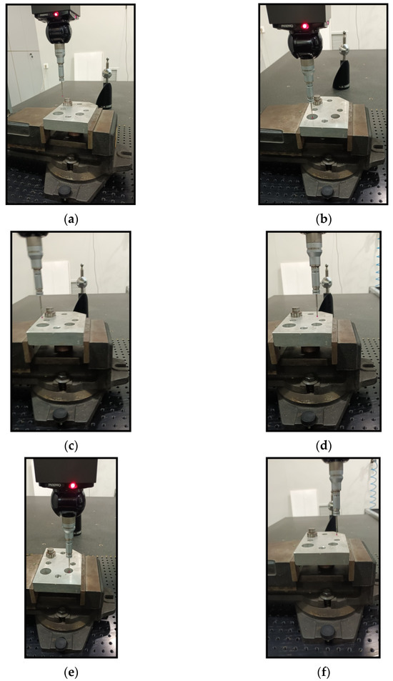
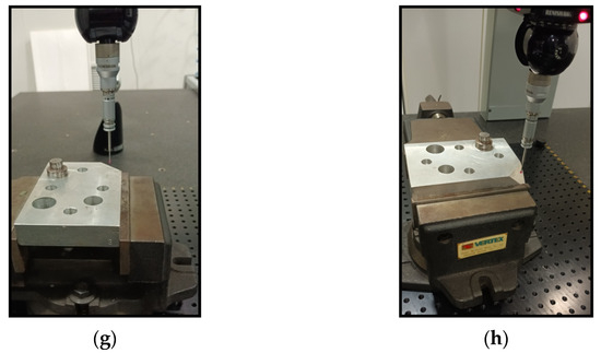
Figure 10.
The resulting path is executed by the CMM: (a–h) depiction of the CMM probe’s spatial location during the path execution.
Figure 11a–d depict the length distribution diagrams of the length per iteration of the formed alternative points sequences. Although the initial total path length is relatively high, the algorithm, after some iterations, converges towards the optimal solution. The length of the resulting path is 327.53 mm. The total computational time for formatting the required paths and solving the TSP was measured at 148.7 s.
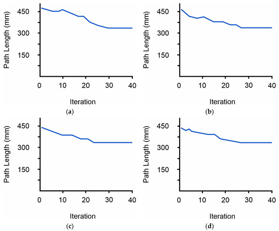
Figure 11.
Diagrams of path lengths per iteration for solving the TSP: (a) Case A for the sequence of inputted points; (b) Case B for the sequence of inputted points; (c) Case C for the sequence of inputted points; (d) Case D for the sequence of inputted points.
The sequence of inputted points does not affect the length of the final solution; it alters the resulting path length per iteration diagram as well as the dynamics of the algorithm’s convergence. This is evident in Figure 11a–d where each diagram was generated from a different inputted sequence of points. The variations in the dynamics of the convergence of the algorithm are not related to the sequence of input points but to its inherent stochastic behavior and the initial values of the parameters. Specifically, the roulette wheel method enables the random selection of all the available options. Even though the possibility of selecting some options is low, they can still be selected. This variability can lead to different convergence patterns.
The presented methodology cannot be compared with some of the state-of-the-art (SOTA) methods due to the fact that SOTAs have not yet been applied by researchers to solve the problem of finding the optimal sequence of measurements using a CMM. Until now, there is no alternative methodology to address the TSP in a complex environment with obstacles. The current approaches are limited to cases where the path length between regions is known without taking into account the existence of obstacles between regions [31]. TSP is applied in fields such as vehicle routing, logistics optimization and various scheduling problems [31]. Its applications in the CMM and measuring operations remain unexplored. More information on the comparison of the AFSA integrating the ray casting algorithm for the generation of the individual paths with the other SOTAs can be found in [27].
Figure 12a and 12b present examples of thin and dense grid environments, respectively. The grid environment in both cases represents a space with the same dimension to ensure the comparability between the results. The starting point is represented in green and the ending point in blue. The environment has dimensions . The grid environment of Figure 12a consists of 192 discrete points, whereas the grid depicted in Figure 12b contains 1536. Each district point represents a volume of in Figure 12a and mm in Figure 12b. The obstacles in both environments represent the same component. In the thin grid, the phenomenon of obstacle overexpansion is strongly observed, especially in the representation of the component’s vertical dimension. It is supported by the fact that, in the thin environment, the vertical dimension is modeled through discrete points corresponding to spatial intervals of 600 mm, while in the dense grid, the same dimension is represented with discrete points of 450 mm. Moreover, the holes of the components in the dense environment are represented with four discrete points, compared to one in the thin grid. The algorithm in both cases has formed the optimal paths. In the case of Figure 12a, the length of the formed path is 2026.2 mm, while for the grid in Figure 12b it is 1668.9 mm. The differences between the lengths of the formatted paths are attributed to the phenomenon of the obstacle’s overexpansion. The computational time for path generation was 13.79 s and 97.24 s for the thin and dense environments, respectively. Figure 12c and 12d presents the diagrams of the formatted path’s length per iteration for the environments in Figure 12a and 12b, respectively. The diagrams reveal that the variation in path lengths is notably lower in the thin environment than in the dense environment. This is attributed to the fact that in the thin environment, the number of discrete points is lower compared to the dense one; as a result the number of alternative paths that can be evaluated is smaller. The zero entries in the diagram of Figure 12c represent paths that concluded in dead-ends and were excluded. The parameters utilized for both environments were identical and their values aligned with those presented at the beginning of the section.
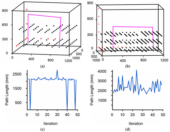
Figure 12.
Path planning in thin and dense grid environment: (a) path planning represented in thin grid environment; (b) path planning represented in dense grid environment; (c) path’s length diagram for thin grid environment; (d) path’s length diagram for dense grid environment.
The examples presented in Figure 12a,b evidence that grid density and object representation accuracy influence the algorithm’s convergence speed and the quality of the final solution. The phenomenon of obstacle overexpansion can be avoided by increasing the density of the grid. The dense grid environments favor a more accurate representation of the pieces, especially in cases where there are curved sections or holes. If the utilized grid is too thin, the curved sections and holes may be represented as distorted or vanish entirely. The density and size of the grid should be chosen to align with the geometric characteristics and dimensions of the represented component.
4. Discussion
This paper presented an approach to reduce the measuring time of a component using an existing CMM without any external interference to the machine or the component. The reduction in components’ measuring time contributes to the acceleration of the manufacturing process and reduces the production costs in an efficient, dynamic and intelligent way, without needing to invest additional funds or resources. The proposed methodology can be applied to any component as long as its CAD file is available in advance.
The measurement time is reduced by optimizing the sequence of measurements. The proposed methodology highlights a novel application of the famous TSP, expanding its scope beyond conventional optimization domains. By tailoring TSP-based optimization to the sequencing of measurements in CMM processes, the study establishes its applicability and value in advanced industrial metrology.
This paper presented the modeling of a component based on its CAD information by appropriately defining the feasible movement points and obstacles in the 3D grid method. Its modeling also takes into account the component’s areas where the measurements will be conducted so that the final results can be executed by the CMM in real-world conditions. An artificial fish swarm algorithm integrated with a ray casting algorithm was successfully modified to meet the requirements of the CMM’s measurement process. The results of the formed 3D paths are used by an ant colony optimization algorithm to solve the Traveling Salesman Problem in a 3D environment with obstacles. The problem’s solution provides the final path and sequence of measurements taking into account the particularities of each component. The final path is also taking advantage of the areas that are located very close to the workpiece and the CMM can move freely without colliding with any part of the manufactured component.
A crucial element for the successful implementation of the presented methodology is the representation of the components in a grid environment. The dimensions and density of the grid impact the algorithm’s convergence rate and the quality of the final path. In thin grids, the phenomenon of obstacle overexpansion may occur, leading to a generalized or less detailed representation of the component’s geometric features. However, thin grids reduce the algorithm’s execution time. In dense grid environments, the phenomenon of obstacle overexpansion is mitigated. They also allow a more accurate precise representation of component geometric characteristics, particularly in the presence of curved profiles or holes. The increased numbers of discrete points in dense grids lead to a longer convergence time for the algorithm. In the examined examples, the algorithm required 85,81% less time in the thin grid to determine the optimal path. Nonetheless, in the dense grid, it generated a path that was 17.63% shorter.
The combination of modeling and algorithms presented in this paper ensures that the final path is the shortest possible and can be applied in real-world conditions. Future research may include the following:
- Advanced grid configuration that dynamically adjusts in some areas;
- Developing a modified AFSA to find the optimal path in a grid environment that is dynamically adjusted in some regions.
Author Contributions
Conceptualization, I.C., G.M., V.P., M.T.M. and A.T.; methodology, I.C., G.M., V.P., M.T.M. and A.T.; software, I.C., V.P. and M.T.M.; validation, G.M. and A.T.; formal analysis, G.M. and A.T.; investigation, I.C., G.M., V.P., M.T.M. and A.T.; data curation, G.M., M.T.M. and A.T.; writing—original draft preparation, I.C., G.M., V.P., M.T.M. and A.T.; writing—review and editing, I.C., G.M., V.P., M.T.M. and A.T.; visualization, I.C., V.P. and M.T.M.; supervision, G.M., M.T.M. and A.T.; project administration, G.M. All authors have read and agreed to the published version of the manuscript.
Funding
This research received no external funding.
Data Availability Statement
Data will be available upon request from the corresponding authors.
Conflicts of Interest
The authors declare no conflicts of interest.
References
- Liu, C.; Wu, L.; Xiao, W.; Li, G.; Xu, D.; Guo, J.; Li, W. An Improved Heuristic Mechanism Ant Colony Optimization Algorithm for Solving Path Planning. Knowl.-Based Syst. 2023, 271, 110540. [Google Scholar] [CrossRef]
- Ab Wahab, M.N.; Nazir, A.; Khalil, A.; Ho, W.J.; Akbar, M.F.; Noor, M.H.M.; Mohamed, A.S.A. Improved Genetic Algorithm for Mobile Robot Path Planning in Static Environments. Expert Syst. Appl. 2024, 249, 123762. [Google Scholar] [CrossRef]
- Fan, H.; Huang, J.; Huang, X.; Zhu, H.; Su, H. BI-RRT*: An Improved Path Planning Algorithm for Secure and Trustworthy Mobile Robots Systems. Heliyon 2024, 10, e26403. [Google Scholar] [CrossRef] [PubMed]
- Diao, X.; Chi, W.; Wang, J. Graph Neural Network Based Method for Robot Path Planning. Biomim. Intell. Robot. 2024, 4, 100147. [Google Scholar] [CrossRef]
- Zheng, X.; Cao, J.; Zhang, B.; Zhang, Y.; Chen, W.; Dai, Y.; Zhao, J. Path Planning of PRM Based on Artificial Potential Field in Radiation Environments. Ann. Nucl. Energy 2024, 208, 110776. [Google Scholar] [CrossRef]
- Rao, J.; Xiang, C.; Xi, J.; Chen, J.; Lei, J.; Giernacki, W.; Liu, M. Path Planning for Dual UAVs Cooperative Suspension Transport Based on Artificial Potential Field-A* Algorithm. Knowl. Based Syst. 2023, 277, 110797. [Google Scholar] [CrossRef]
- Wdowik, R.; Magdziak, M.; Ratnayake, R.M.C.; Borsellino, C. Application of Process Parameters in Planning and Technological Documentation: CNC Machine Tools and CMMs Programming Perspective. Procedia CIRP 2018, 78, 43–48. [Google Scholar] [CrossRef]
- Soni, J.; Pantawane, P.D. Review Paper on Probing System of CMM; COPEN: San Francisco, CA, USA, 2019. [Google Scholar]
- Dhanish, P.B.; Mathew, J. Effect of CMM Point Coordinate Uncertainty on Uncertainties in Determination of Circular Features. Measurement 2006, 39, 522–531. [Google Scholar] [CrossRef]
- Sadaoui, S.E.; Mehdi-Souzani, C.; Lartigue, C.; Brahim, M. Automatic Path Planning for High Performance Measurement by Laser Plane Sensors. Opt. Lasers Eng. 2022, 159, 107194. [Google Scholar] [CrossRef]
- Morozov, M.; Pierce, S.G.; MacLeod, C.N.; Mineo, C.; Summan, R. Off-Line Scan Path Planning for Robotic NDT. Measurement 2018, 122, 284–290. [Google Scholar] [CrossRef]
- Masood, A.; Siddiqui, R.; Pinto, M.; Rehman, H.; Khan, M.A. Tool Path Generation, for Complex Surface Machining, Using Point Cloud Data. Procedia CIRP 2015, 26, 397–402. [Google Scholar] [CrossRef]
- Fountas, N.A.; Vaxevanidis, N.M. Intelligent 3D Tool Path Planning for Optimized 3-Axis Sculptured Surface CNC Machining through Digitized Data Evaluation and Swarm-Based Evolutionary Algorithms. Measurement 2020, 158, 107678. [Google Scholar] [CrossRef]
- Lin, X.; Jiang, S.; Liu, X.; Yang, K. The CMM Measurement Path Planning for Blade Surface Based on the Contour Measurement. In Proceedings of the 2011 2nd International Conference on Digital Manufacturing and Automation, ICDMA 2011, Zhangjiajie, China, 5–7 August 2011; pp. 1228–1232. [Google Scholar] [CrossRef]
- Stojadinovic, S.; Majstorovic, V.D.; Durakbasa, M.N. A Feature—Based Path Planning for Inspection Prismatic Parts on CMM. In Proceedings of the XXI Imeko World Congress, Prague, Czech Republic, 30 August–4 September 2015. [Google Scholar]
- Wan, N.; Jiang, R.; Zhao, H.; Zhang, S. An Inspection Path Optimization of Impeller for Balancing Efficiency and Accuracy. Measurement 2019, 141, 472–485. [Google Scholar] [CrossRef]
- Ma, D.; Ma, T.; Li, Y.; Ling, Y.; Ben, Y. A Contour-Based Path Planning Method for Terrain-Aided Navigation Systems with a Single Beam Echo Sounder. Measurement 2024, 226, 114089. [Google Scholar] [CrossRef]
- Mansour, G.; Sagris, D.; Tsagaris, A. CMM Path Planning, Position and Orientation Optimization Using a Hybrid Algorithm. Int. Rev. Mech. Eng. (IREME) 2017, 11, 144. [Google Scholar] [CrossRef]
- Jin, X.; Yan, Z.; Yang, H.; Wang, Q. A Practical Sampling-Based Motion Planning Method for Autonomous Driving in Unstructured Environments. IFAC-PapersOnLine 2021, 54, 449–453. [Google Scholar] [CrossRef]
- Ou, J.; Hong, S.H.; Song, G.; Wang, Y. Hybrid Path Planning Based on Adaptive Visibility Graph Initialization and Edge Computing for Mobile Robots. Eng. Appl. Artif. Intell. 2023, 126, 107110. [Google Scholar] [CrossRef]
- Li, P.; Chen, D.; Wang, Y.; Zhang, L.; Zhao, S. Path Planning of Mobile Robot Based on Improved TD3 Algorithm in Dynamic Environment. Heliyon 2024, 10, e32167. [Google Scholar] [CrossRef] [PubMed]
- Huang, S.; Chen, W.; Lu, B.; Xiao, F.; Shen, C.; Zhang, W. An Improved BAT Algorithm for Collaborative Dynamic Target Tracking and Path Planning of Multiple UAV. Comput. Electr. Eng. 2024, 118, 109340. [Google Scholar] [CrossRef]
- Huang, H.; Shang, Y.; Liu, X.; Liu, X.; Qi, P. An Improved Bi-RRT*-Based Path Planning Algorithm with Adaptive Search Strategy Assignment Mechanism for Ultra-Low-Altitude Penetration of Fixed-Wing Aircraft. Aerosp. Sci. Technol. 2024, 152, 109363. [Google Scholar] [CrossRef]
- Zhou, Y.; Su, Y.; Xie, A.; Kong, L. A Newly Bio-Inspired Path Planning Algorithm for Autonomous Obstacle Avoidance of UAV. Chin. J. Aeronaut. 2021, 34, 199–209. [Google Scholar] [CrossRef]
- Chowdhury, A.; De, D. RGSO-UAV: Reverse Glowworm Swarm Optimization Inspired UAV Path-Planning in a 3D Dynamic Environment. Ad Hoc Netw. 2023, 140, 103068. [Google Scholar] [CrossRef]
- Mansour, G.; Chouridis, I.; Tsagaris, A. Finding the Optimal Path in a 3D Environment with Predefined Obstacles. Int. J. Adv. Mechatron. Syst. 2024, 11, 50–62. [Google Scholar] [CrossRef]
- Chouridis, I.; Mansour, G.; Papageorgiou, V.; Mansour, M.T.; Tsagaris, A. Enhanced Hybrid Artificial Fish Swarm Algorithm for Three-Dimensional Path Planning Applied to Robotic Systems. Robotics 2025, 14, 32. [Google Scholar] [CrossRef]
- Chouridis, I.; Mansour, G.; Tsagaris, A. Three-Dimensional Path Planning Optimization for Length Reduction of Optimal Path Applied to Robotic Systems. Robotics 2024, 13, 178. [Google Scholar] [CrossRef]
- Neshat, M.; Sepidnam, G.; Sargolzaei, M.; Toosi, A.N. Artificial Fish Swarm Algorithm: A Survey of the State-of-the-Art, Hybridization, Combinatorial and Indicative Applications. Artif. Intell. Rev. 2014, 42, 965–997. [Google Scholar] [CrossRef]
- Poudel, S.; Arafat, M.Y.; Moh, S. Bio-Inspired Optimization-Based Path Planning Algorithms in Unmanned Aerial Vehicles: A Survey. Sensors 2023, 23, 3051. [Google Scholar] [CrossRef] [PubMed]
- Matai, R.; Singh, S.; Lal, M. Traveling Salesman Problem: An Overview of Applications, Formulations, and Solution Approaches. In Traveling Salesman Problem, Theory and Applications; IntechOpen: London, UK, 2010. [Google Scholar] [CrossRef]
Disclaimer/Publisher’s Note: The statements, opinions and data contained in all publications are solely those of the individual author(s) and contributor(s) and not of MDPI and/or the editor(s). MDPI and/or the editor(s) disclaim responsibility for any injury to people or property resulting from any ideas, methods, instructions or products referred to in the content. |
© 2025 by the authors. Licensee MDPI, Basel, Switzerland. This article is an open access article distributed under the terms and conditions of the Creative Commons Attribution (CC BY) license (https://creativecommons.org/licenses/by/4.0/).