Abstract
Metrological traceability is essential for ensuring the accuracy of measurement results and enabling a comparison of results to support decision-making in society. This paper explores a structured approach to modelling traceability chains, focusing on the role of residual measurement errors and their impact on measurement accuracy. This work emphasises a scientific description of these errors as physical quantities. By adopting a simple modelling framework grounded in physical principles, the paper offers a formal way to account for the effects of errors through an entire traceability chain, from primary reference standards to end users. Real-world examples from microwave and optical metrology highlight the effectiveness of this rigorous modelling approach. Additionally, to further advance digital systems development in metrology, the paper advocates a formal semantic structure for modelling, based on principles of Model-Driven Architecture. This architectural approach will enhance the clarity of metrological practices and support ongoing efforts toward the digital transformation of international metrology infrastructure.
1. Introduction
Traceability is a fundamental concept in metrology. Quantities must be expressed on a metrologically traceable measurement scale to enable meaningful comparison. For this reason, traceability is critical to the functioning of international quality infrastructures (QIs) and to the dissemination of measurement units within the global measurement system [1]. Also for this reason, traceability is often mandated when critical decisions depend on measurements of physical quantities.
A pair of international arrangements that rely on traceability have been established. These arrangements have fostered the development of national and international quality infrastructure, which provides access to necessary traceable measurement services in society. In 1999, the International Committee for Weights and Measures (CIPM) Mutual Recognition Arrangement (MRA) provided a framework for national metrology institutes (NMIs) to demonstrate the equivalence of their measurement capabilities to those of international peers [2]. Similarly, in 2001, the International Laboratory Accreditation Cooperation (ILAC) multi-lateral MRA provided a framework to support the provision of calibration and testing services across the developed world [3].
The concept of traceability emerged late in the 20th century [4]. Four possible definitions for traceability were considered in an early paper by Belanger [5,6]. In 1982, Nicholas and White, in their monograph Traceable Temperatures, proposed a variation on one of Belanger’s suggestions [7]. Then, in 1984, the first edition of the Vocabulary of Metrology (VIM) included an entry for traceability, drawing on another of Belanger’s suggestions ([8], 6.12). Later editions of the VIM expanded and refined the definition of traceability. The second edition, in 1993, emphasised that traceability was a quantitative characteristic of measurement by including reference to uncertainty ([9], 6.10). This revision coincided with the release of the first edition of the Guide to the Expression of Uncertainty in Measurement (GUM) [10]. The current definition of traceability in the third edition of the VIM is as follows ([11], 2.41):
metrological traceability
This incorporates terms with specific meanings—measurement result, calibration, and measurement uncertainty—which are also defined in the VIM. The definition is accompanied by eight explanatory notes, one of which elaborates on the meaning of reference.property of a measurement result whereby the result can be related to a reference through a documented unbroken chain of calibrations, each contributing to the measurement uncertainty.
It is notable that the definition of traceability includes a requirement for documentation. Metrology is a scientific discipline, and traceability is one of its fundamental principles. It is unusual to see such a practical requirement being specified in a scientific definition. However, traceability plays the functional role in society of ensuring the reliability of measurements. The need for documentation stems from the real-world requirement to audit the reliability of the measuring stages along a traceability chain. Thus, the VIM definition integrates both the scientific concept of traceability and the practical necessity of generating records that can be audited.
The term “traceability” encompasses a range of meanings. As De Biève notes, “traceability is a general (superordinate) concept” [12]. The description of metrological traceability in the VIM is a specialised interpretation. The VIM associates traceability with measurement uncertainty; however, it is beneficial to distinguish between them. De Biève opines that traceability is a prerequisite for the evaluation of measurement uncertainty [13]; thus, measurement uncertainty cannot be meaningfully assessed without first establishing traceability—a view shared by Ehrlich and Rasberry [14]. This highlights the importance of structure—or configuration—in traceability: the way in which stages in a traceable measurement are designed to provide a link back to a metrological reference.
In this article, we emphasise the importance of modelling such configurations and suggest that this task should be clearly distinguished from the evaluation of uncertainty; however, in practice, they are often conflated. For example, Cox and Harris describe the evaluation of uncertainty as comprising two phases: first, the formulation of a model; and second, its evaluation [15]. They emphasise that the first phase must be carried out by metrologists, to identify and capture all relevant information, whereas the second is a computational task. The GUM and its supplements also presuppose a mathematical model of the measurement has been formulated [16]. We agree with Cox and Harris that model formulation is the responsibility of the metrologist. However, we stress that this should involve modelling of the physical measurement. The calculation of uncertainty will ultimately use information from this model to construct a suitable computational form—a process that might itself be viewed as a kind of modelling by a statistician, because abstract statistical concepts may be introduced. We believe that maintaining a clear separation between measurement modelling and the evaluation of uncertainty is beneficial.
The international metrology community has recently embarked on a digital transformation of its systems and processes, which may entail substantial change [17]. This initiative is motivated by a belief that significant gains in efficiency and reliability can be achieved. However, designing a digital infrastructure that simply automates the various tasks that people perform today is unlikely to foster innovation. Metrology is practised by skilled professionals throughout the world’s quality infrastructures, whose work is shaped by their interpretations of authoritative documents like the VIM and GUM. The implementation details can vary—between organisations, between economies, and between regional metrology organisations. This diversity will complicate an overarching digitalisation of quality infrastructure activities, as neither the analysts eliciting business requirements nor the metrologists describing their work have explicit guidance about the balance between practical considerations and scientific requirements. For example, the definition of traceability does not explain the purpose for measurement uncertainty or why documentation is needed [18]. These important aspects are left to the discretion of metrologists.
This article examines traceability as a fundamental scientific principle and advocates for explicit measurement modelling, which provides direct and valuable insights into how various types of measurement achieve traceability. Starting with a few basic assumptions, we show that measurements can be modelled with mathematical expressions. These models can represent the influence quantities that ultimately determine the accuracy of measurement results at the end of a traceability chain. Traceability is established by accounting for these influences; indeed, the elements that need to be “traced” along a metrological traceability chain are the residual measurement errors arising from uncontrolled influences. Mathematical notation provides a concise, consistent, and logical structure, offering several advantages: it transcends linguistic differences, is widely understood, and facilitates rigorous analysis.
The structure of this article is as follows. The next section introduces some foundational assumptions and a notation for measurement modelling. Section 3 illustrates modelling in a variety of scenarios, including ratio and difference measurements, international comparisons, intrinsic and quantum-based standards, and sensor networks. Section 4 examines the possibility of evaluating models and establishes a connection between modelling and the calculation of measurement uncertainty. Section 5 examines a way of structuring semantic model information to better align scientific concepts with digital systems development. This approach will facilitate the digitalisation of metrological processes and enhance interoperability. Section 6 discusses our contention that residual measurement error is central to a scientific description of traceability. It highlights examples from microwave metrology, optical goniometry and an international measurement comparison where modelling has improved measurement accuracy and information flow along traceability chains. Our conclusions are summarised in Section 7, which is followed by three appendices. Appendix A develops a model for calibrating a simple linear measuring system, Appendix B summarises a method for evaluating measurement uncertainty as described in the original GUM, and Appendix C outlines a method for evaluating uncertainty provided in supplements to the GUM.
2. Modelling
2.1. Basic Assumptions and Notation
A few simple assumptions provide a foundation for modelling. The first is that the quantity intended to be measured can, for all practical purposes, be uniquely defined. This quantity is called the measurand ([16], 3.1.3). A second assumption is that the measurand cannot be determined exactly; the value obtained by measurement is an approximation—an estimate—of the measurand. Consequently, since the exact value of the measurand is unknowable, the deviation of a measured value from the measurand cannot be determined either. Nevertheless, the best estimate of this deviation is usually zero (It is generally assumed that any known effect causing bias in a measurement will be corrected, ensuring that the measured value remains unbiased).
These assumptions suggest three entities for modelling measurements. Our notation distinguishes between them (if conventional notation in a technical discipline cannot be easily reconciled with the one proposed here, unknown-value terms may be underscored (e.g., ) rather than capitalised):
- 1.
- A known value—such as the indication of a measuring system—is denoted by a lower-case italicised term (e.g., y);
- 2.
- An unknown value—such as a measurand—is represented by an upper-case italicised term (e.g., Y); and
- 3.
- An unknown residual value that has an estimate of zero—such as the difference between a measured value and the measurand—is denoted by an upper-case italic E and a suitable subscript to label the term (e.g., ).
In this notation, the second assumption above—that a measurand cannot be determined exactly—may be expressed simply as
where Y represents the measurand, y is its estimate, and the difference between them is the residual error term . The subscript of corresponds to the estimate of the measurand, because a different estimate would yield a different residual value.
2.2. Static Models
A measurement model is an equation that expresses a measurand in terms of the other definite quantities involved in a measurement. Equation (1) is the most general form of a measurement model, comprising only two quantities: the (known) measured value and the (unknown) difference between that value and the measurand. The equation expresses the fact that the measurand’s value could be determined if the residual measurement error were known. It shows that determines the accuracy of the measured value y as an approximation of the measurand Y. In practice, information about the likely magnitude of is attributed to the measurement uncertainty associated with the measured value, y.
Note that this model provides a static view of what occurs during a measurement. Each term represents a definite quantity, although some values are not known. This is analogous to a coin toss where the outcome remains covered by a hand: the result is definite but unknown to observers. A static representation does not inherently distinguish between systematic and random measurement errors, so careful consideration is sometimes required to avoid ambiguity when developing models and assigning identifiers to model terms. For example, if a measurement is affected by a random error, the corresponding term may include an instance identifier. The residual random error in the ith measurement could be denoted , where i serves to distinguish individual instances as needed.
2.3. Model Building
Modelling provides a quantitative framework to describe measurement results. Model construction is guided by the intended purpose. The level of detail required in a model depends on the information desired about a measurement. Since no measurand can be determined exactly, Equation (1) serves as a generic model applicable to any measurement. However, it provides no insight into the quantities influencing the measurement result. An essential part of metrologists’ work is to identify the influence quantities that affect a measurement and incorporate these factors into a model, which can be analysed to evaluate the measurement uncertainty. Such models usually have many terms. However, between the extremes of a completely generic model and one describing a specific measurement in detail, models with just a few terms that summarise a measurement result can also be employed. For instance, it may be convenient to represent the combined effect of numerous random influence factors using a single term, while modelling systematic errors individually [19]. For example, when two systematic effects, A and B, influence each measurement of Y, a suitable model could be
where represents the combined effect of random errors in the ith measurement of Y.
2.4. Traceability
The accuracy of information obtained by measurement at the end of traceability chains is critical. It must be possible to assess whether the measurement accuracy available is fit for purpose in a given context. Along a chain, the accuracy of measuring systems must be accounted for to assess the likely magnitude of residual measurement error at each stage. That is why national metrology institutes invest significant resources in developing and maintaining realisations of measurement scales for SI base units and other related quantities, known as primary measurement standards. These standards provide the initial stage in the dissemination of units of measurement; they anchor traceability chains, so reliable information can be obtained later at their endpoints.
Calibration is the metrological process used to disseminate measurement units along a traceability chain. It characterises a measuring system and enables measured values to be traced back to calibration standards, and ultimately to primary standards. Calibration is carried out in two distinct phases ([11], 2.39). First, the response of the system being calibrated to certain reference standards is determined. This information is then used in the second phase to establish a relationship describing the system’s response to an unknown measurand—in other words, to construct a measurement model. The two phases are distinct in their modelling requirements. The first focuses on the behaviour of the measuring system and requires a model that can explain non-ideal behaviour. During this phase, the model terms that characterise non-ideal behaviour are measured. The second phase establishes a measurement model which incorporates the terms measured in the first phase.
A simple example helps to illustrate these ideas. The behaviour of a mass balance is modelled by a systematic effect, O, which offsets balance readings, and a random error, , which represents the inherent variability of repeated balance readings. The ith balance indication is
where M is the mass being measured. Equation (3) describes the behaviour of the measuring system, but it is not a measurement model. The system response is the focus of this equation, which is sometimes referred to as an observation equation.
In the first phase of calibration, a measure of the fixed offset can be obtained by looking at the response of the balance to a mass standard. This mass,
is not exactly known, but when placed on the balance, the indication is
Rearranging, we obtain a measurement model for the offset
The measured value of O is the difference between the balance indication, , and a reported value of the mass standard, . This is associated with two components of error: one due to the repeatability of the balance and another associated with the accuracy of the value, , attributed to . The offset O may be summarised for modelling as
where
In the second phase of calibration, a measurement model for the calibrated balance can be established, which incorporates the information about its offset. The model relates a balance indication, , to the measurand,
Equation (10) involves two measurement stages along a traceability chain: one is a determination of the reference mass, ; the other is a measurement of some mass, M, using the calibrated balance. Calibration of the system makes a connection between these two stages. The residual error in the value , which is an estimate of M, has three components, one of which is from the previous stage. Thus, to properly account for measurement error in M, we should also know about the measurement error in the calibration standard used.
Although not shown in the example, traceability requires links to be created all the way up the chain to a primary standard or suitable reference. Here, inherently depends on other measuring systems, unless the measurement of was performed using a primary mass standard. These other measuring systems must be calibrated too. This reflects the nature of a traceability chain, in which documented auditable links are forged by successive calibrations.
2.5. Topology
Traceability chains are not necessarily simple linear structures linking one measurement stage to the next. Chains can divide into multiple branches and continue to grow through independent calibrations and measurement processes. They may also merge, either as independent chains converging or as previously divided branches recombining.
With careful labelling of terms, modelling can represent these structures, enabling thorough analysis. For instance, consider two masses, and , weighed using the same calibrated balance. The individual measurements can be modelled as:
These are independent branches; however, if we are interested in the mass difference, , the branches recombine when the difference is evaluated. Subtracting (12) from (11) and simplifying, we obtain a model for the difference measurement,
The individual mass readings are correlated by terms associated with calibration; however, Equation (13) shows these shared effects do not influence the mass difference measurement.
Modelling can capture variations of this scenario. Suppose, the same mass reference is used to calibrate the balance before each measurement (see Figure 1). To distinguish the influence quantities arising during these calibrations, we write:
where “” labels quantities from one calibration, and “” labels those from the other. The mass difference is now
The quantities arising in balance calibrations no longer cancel; however, the mass difference measurement remains insensitive to the mass calibration standard.
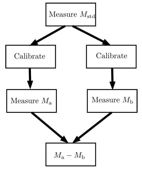
Figure 1.
A measurement of mass difference offers an example of a traceability chain that divides and later recombines. The chain bifurcates when a mass balance is calibrated using the same mass, , before each measurement. Distinct influence quantities arise during these calibrations and the mass measurements that follow, but the influences associated with the determination of are shared and correlate the individual mass measurements. The chains combine when the mass difference is evaluated.
An intriguing outcome in these examples is the apparent insensitivity of the difference measurement to the mass standard used for calibrating the balance: it seems that a traceable calibration standard is unnecessary. However, this conclusion arises from the simple model adopted for the measuring system, which provides a very basic representation of the balance. This issue is revisited in Section 3.2.
3. Different Traceability Scenarios
The principal argument of this article is that physical modelling can describe the relationship between a measurand and a measured value of that measurand. The measurand is a defined quantity, whereas a measured value is the outcome of a real-world process (a measurement) influenced by various physical factors. The challenge lies in finding a suitable model to represent the relationship between a measured value and the measurand in different situations.
3.1. Quantity Ratios
Mathematical measurement models must adhere to the rules of quantity calculus and the laws of physics. One such rule is that, for terms to be legitimately added or subtracted, they must represent quantities of the same kind. Therefore, only quantities of the same kind can be compared by difference. On the other hand, there is no such restriction on the multiplication and division of quantities. A product of quantities is understood to be proportional to its various factors. Thus, the ratio of two quantities of the same kind is sometimes said to be “dimensionless”, meaning that the ratio does not depend on the units used to express values in the numerator and denominator.
This raises an interesting question about traceability: what is an appropriate reference to establish traceability when a measurand is the ratio of two quantities of the same kind? Before addressing this, it is important to clarify a potential source of confusion. In dimensional analysis, dimensionless quantities are treated as pure numbers, which is convenient for mathematical analysis of dimensional problems; however, this is not appropriate when modelling measurements. Quantities defined as ratios of the same kind of quantity should be regarded as distinct quantities in their own right. For example, the linear scale factor, which is a ratio of lengths, is clearly not the same as emissivity, which is a ratio of energies.
When a measurand is defined as the ratio of quantities, there are two possible approaches to establish traceability to an appropriate reference, thereby anchoring the traceability chain. One approach is to trace back to a primary standard for the ratio quantity itself; the other is to trace back to standards for the individual quantities in the numerator and denominator (This is not limited to ratios of the same kind of quantity. For instance, measurements of speed can be traced back to standards of length and time). The first case is no different from establishing traceability to any quantity for which a reference of the same kind is available; the traceability chain can be straightforwardly modelled back to a primary standard.
The second case can be affected by common factors associated with the traceability chains of the numerator and the denominator. For instance, using the same system to measure both quantities may result in the cancellation of some terms. Nevertheless, it is important to consider the situation carefully. Appendix A describes an example where a linear system measures the ratio of two quantities, and . The measurement model, given in Equation (A6), is
where G is a gain factor, and O is a fixed offset. The gain factor cancels in the model of the ratio measurement (A11):
However, during calibration, the measured value of the offset (A5) is actually influenced by the system gain. Equation (A12), in the appendix, provides an expression for the ratio measurement model that shows how traceability is derived from the standards used to calibrate the system. Thus, the traceability of a measurement of the ratio of Q is established through traceability chains that refer back to Q for both the numerator and the denominator.
3.2. Quantity Differences
In Section 2.5, a simple mass balance was used to show how calibration creates links between the stages of a traceability chain. However, we noted that the chain was abruptly truncated when the balance was incorporated into a model of a mass difference measurement. In fact, the balance’s representation was quite simple: it accounted for a fixed offset and a repeatability error but assumed a perfect response to mass increments. This model allowed the balance to be calibrated by just measuring its offset. Since an offset does not affect the measurement of a mass difference, the representation effectively truncated the traceability chain for a mass difference.
A better representation of a balance could take account of the sensitivity, or gain, of its response to different masses. One way to do this is to introduce a gain factor, G, to the original model. The observation equation for an indication is then
where M, O, and represent the measurand, offset, and random error, respectively, as before. The parameters G and O must be determined by calibration, which requires at least two calibration standards, and (Appendix A gives the calibration equations for a generic linear system measuring Q, rather than M).
The mass difference measurement model is now
which does not depend on the balance offset. However, the measurement model of G used during calibration depends on and . Thus, the traceability of mass difference measurements using this model would be established in terms of the balance response to changes in mass.
3.3. Measurement Comparisons
As noted in the Introduction, the CIPM MRA [2] provides reliable quantitative information on the metrological compatibility of similar calibration and measurement services at different NMIs. To maintain entries in the MRA, NMIs are expected to participate regularly in international measurement comparisons relevant to their services [20]. In these CIPM key comparisons, a group of NMIs each measure a suitable measurand—often a stable property of an artefact—and then the comparison coordinator applies an agreed method of analysis to the results.
Comparison analyses can assess the reliability of participants’ measurement capabilities. For a measurand Y, participant “a” submits a result , participant “b” submits a result , and so on, with each result accompanied by a corresponding statement of uncertainty. In modelling terms, it may be assumed that , , and so forth, where the residual errors represent the extent to which each result deviated from the measurand. A comparison analysis estimates the residuals , , etc., which are called degrees of equivalence (DoEs). DoEs can be compared with the uncertainty information provided for each result by the participants. If a DoE is larger than can be explained by a statistical interpretation of the uncertainty, it suggests a problem with the participant’s measurement analysis. Likely, some sources of measurement error have not been properly accounted for in the measurement model.
After a CIPM key comparison has been completed, similarly structured RMO key comparisons can be carried out by regional metrology organisations (RMOs). Participation in RMO comparisons gives many more NMIs the opportunity to register and maintain claims under the MRA. To evaluate NMI performance across all comparisons, each RMO comparison must include several participants from the initial CIPM comparison. The systematic effects associated with measurements made by these linking participants introduce correlations in the results. However, such linking effects can be accounted for when measurement models are combined with the algorithms used for comparison analysis. This is described in a report on the analysis methods recommended by the Consultative Committee on Photometry and Radiometry (CCPR) [21]. Succinct measurement models, using one residual error term to represent combined random effects and one to represent combined systematic effects, were used in that analysis. More detailed measurement models, representing the various influence quantities of each comparison participant, can be handled using specific data processing that is designed to evaluate a digital representation of measurement models [22]. Doing so provides more insights into the comparison analysis outcomes.
3.4. Traceability of Intrinsic and Quantum-Based Standards
Intrinsic measurement standards are standards based on an inherent and reproducible property of a phenomenon or substance ([11], clause 5.10). They serve as metrological references with assigned consensus values, such as the triple point of water.
From a modelling perspective, a measurement involving an intrinsic standard can be represented by the generic model (1),
where the single term represents the combined effects of all influence quantities. This term can be expanded into an appropriately detailed model of the realisation of a particular standard. It is recognised that there are generally two sources of uncertainty in the realisation of an intrinsic standard: one associated with the consensus value (common to all realisations) and the other associated with the specific implementation. In modelling terms, this means that an intrinsic standard may have an error that is common to all standards of the same type, arising from the process that fixed a consensus value (an estimate). A second, implementation-specific error, results from influence factors in the realisation of a system.
Comparison with other standards provides evidence that the system in question is adequately represented by its model—that no unaccounted-for influences introduce bias or reduce precision—and that it is metrologically compatible with the measurand. The need to compare systems is fundamentally the same as for the metrology comparisons, described in Section 3.3. To claim traceability, the metrological compatibility of realisations must be demonstrated. Without such verification, traceability cannot be assured [23].
Quantum-based standards are a type of intrinsic measurement standard. These standards rely on the realisation of certain physical properties with well-defined values determined by quantum mechanical phenomena, such as the Josephson effect or the quantum Hall effect. The need for calibration to establish traceability in such systems is seemingly unnecessary. However, their realisation is not immune to influence factors, and so careful characterisation is required, and comparison with independently verified systems is necessary [24].
3.5. Traceability in Sensor Networks
Sensor networks are multiple interconnected systems of sensors, which monitor physical parameters in their environment and transmit data to a central system for aggregation and analysis. The complex topology of many sensor networks presents challenges in establishing metrological traceability. The typical hierarchical structures, where measurement standards and calibrations are used to disseminate traceability, are not easily applied to sensor networks.
Measurement modelling can help by representing sensor measurement results. For example, when sensors are manufactured in large numbers as batches, the characteristics of a batch can be estimated from a smaller sample. This characterisation can be done using traceable measuring systems. The data obtained could be incorporated in sensor models, with batch characteristics represented by common terms for all sensors, sample variability between sensors represented by sensor-dependent fixed-effect terms, and, lastly, variability between repeat observations with individual sensors represented by random effect terms. Errors due to sampling variation could also be included. Modelling in this way allows the data processing to account for systematic effects, enabling the extraction of more precise information from aggregated measurements [25]. Many modern sensors are equipped with data processing capabilities, so sensor models could be integrated in the devices to provide plug-and-play functionality.
4. Model Evaluation
Having mathematical models that represent measurement results raises an important question: can the models be evaluated? Although all terms are assumed to have definite values, some remain unknown, making the computational task seem ill-defined. Nevertheless, terms that are not exactly known can be expressed as the sum of a (known) estimate and an (unknown) residual error. In this form, models can be evaluated by taking zero as the estimate for all residual error terms. This calculation yields the measured value—the best estimate of the measurand.
However, residual measurement errors determine the ultimate accuracy of measured values, which must be accounted for when reporting traceable measurement results. These error terms should not be overlooked. They are the subjects of interest in an evaluation of measurement uncertainty.
In metrology, measurement uncertainty is quantified using probabilistic concepts. However, since probability can be interpreted in different ways, so too can uncertainty. The frequentist interpretation, where probability represents the long-run relative frequency of events, is likely familiar to most readers and is consistent with the GUM [16]. However, the Bayesian view, which is based on a state of knowledge, has been emphasised in later supplements to the GUM [26,27].
While exploring the consequences of adopting different definitions of probability—and, by extension, uncertainty—is beyond the scope of this article, this section focuses on how static measurement models can be used as a foundation for uncertainty calculations. The modelling approach described here is grounded in general physical principles, providing a robust framework for the description of measurements. Decisions about data handling—such as the choice of an appropriate probability interpretation—can be made at the end of a traceability chain based on the type of information required.
4.1. Traceability Chains
A traceability chain consists of a succession of carefully linked stages. While we may say that a “measurement” is performed at each stage, it is the combination of stages that constitutes the actual traceable measurement. The hierarchy of stages along a traceability chain is often depicted in the form of a pyramid or triangle. At the summit are the formal definitions of quantities, implemented directly below by NMIs. Second-tier calibration laboratories then provide calibration services to testing laboratories and industry organisations. As one moves down the hierarchy, traceability chains divide into more and more branches.
At the base, information is gathered about a quantity of interest and used—rather than being passed on—to make a decision. Typically, the final stage compares measured values with other measured values, or with nominal quantities. Comprehensive modelling captures the potentially complex branching structures that can arise—for example, the cases of ratio and difference measurements already mentioned and the complexities of measurement comparison analysis. Representing the complete traceability chain is essential for properly assessing the accuracy of results.
To discuss the staged nature of traceability chains, we adopt specific notation. The interpretation of upper- and lower-case terms follows the meanings provided earlier. To represent a model at a given stage, we use functional notation with a stage-index parameter, such as
where k labels the stage, is the measurand at that stage, and the elements of the set are the arguments of . These arguments may include known and unknown terms evaluated at earlier stages, as well as individually identified quantities or quantity estimates. A complete measurement model is represented by iteration through the stages:
with the final stage delivering the measurand, . It is worth noting that the mathematical composition of stage functions is implicit in this description: later stages are composed of earlier stages.
For instance, if the first and second stage results feed into a third stage, which, in turn, feeds the fourth (Figure 2), the model could be expressed at the fourth stage as
which explicitly shows the composition, while omitting other arguments.
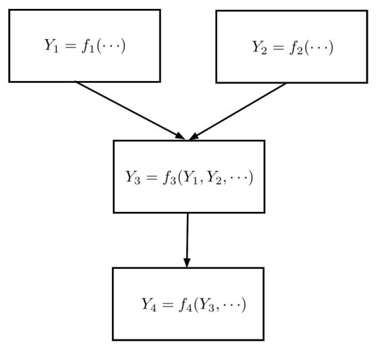
Figure 2.
In general, the results from earlier stages of a traceable measurement are the arguments of later stage models. In this example, the first two stage results are needed during the third stage.
4.2. GUM Evaluation of Uncertainty
The GUM describes a method for evaluating measurement uncertainty when a function describing the measurement is available of the form
where the output quantity Y is the measurand, and are input quantities on which Y depends. A summary of this method is given in Appendix B. The GUM notation is compatible with the notation employed in this paper but is less strict, because capital letters can also denote random variables—an abstract mathematical concept.
Uncertainty arises because the values of some terms in the model are not known exactly. These terms correspond to the input quantities in Equation (22). To evaluate the uncertainty of y as an estimate of Y, additional information about the input quantities is required. Specifically, denotes the standard uncertainty of the estimate, , of , expressed as a standard deviation, while represents the degrees of freedom associated with . Furthermore, if there is correlation between estimates, the correlation coefficient must be provided. Models developed using the approach described in this paper can be handled by the GUM methodology when values for these attributes are documented with the model.
The application of the GUM treatment of uncertainty to static models implies a frequentist interpretation of probability, where the variability of the data is associated with influence quantities. The GUM classifies methods for evaluating the uncertainty of input quantities into two groups: Type A, which applies statistical evaluation methods to data obtained during the measurement, and Type B, where information is obtained outside the measurement. Standard methods for evaluating sample statistics are typically used in Type A data processing and are rooted in classical frequentist approaches. Type B evaluation draws on other sources of information, such as a physical model of a process that influences the measurement. This Type B analysis aligns with the view that terms represent observable quantities that vary due to physical effects. Consequently, a frequentist interpretation of probability is also applicable for Type B uncertainties.
While it is sometimes argued that systematic errors complicate the frequentist analysis of a measurement, static modelling removes this concern. Static models do not differentiate between random and systematic errors. A static model represents all the quantities that contributed to a measurement result, with each having a definite value that may or may not be known. Influences typically classified as systematic are represented by single terms with enduring values, whereas influences typically classified as random are represented by multiple terms, each with a value associated with a different part of a measurement. In this way, static models capture the effects typically ascribed to systematic errors, as demonstrated in the simple cases of difference and ratio measurements in Section 3.2 and Section 3.1.
4.3. The Monte Carlo Method for Evaluating Uncertainty
A Monte Carlo simulation has many applications in computational science. It is commonly used to model dynamic stochastic behaviour, providing insights into how a system evolves over time. The Joint Committee on Guides in Metrology (JCGM) has issued supplements to the GUM that describe a method of computing uncertainty called the Monte Carlo Method (MCM) [26,27]. However, this method does not model dynamic system behaviour ([26], Note 2, p. 10). Instead, random number generation is used to evaluate Bayesian probability distributions associated with unknown fixed quantities. A brief summary of the MCM is given in Appendix C.
As explained in Section 4.2, the GUM notation is compatible with the notation employed in this paper. Thus, models developed using the approach described here can serve as precursors to MCM uncertainty calculations. Additional information about the input quantities in Equation (22) is required. These terms are associated with probability distributions representing the state of knowledge about the inputs, and the result of an MCM calculation represents the state of knowledge distribution for the output quantity Y. The interpretation of uncertainty statements produced by the MCM is different from uncertainty statements produced using the GUM method. Applying the MCM treatment of uncertainty implies a Bayesian interpretation of probability, which is not based on the variability of the data, i.e., relative frequency ([26], Note 4, p viii).
As with the GUM method, the static modelling of the full traceability chain facilitates the formulation of MCM calculations because the distinction between random and systematic errors is unnecessary. Static modelling uniquely identifies all quantities instead of classifying some as random and others as systematic. Within the context of an MCM calculation, model terms correspond to specific realisations of random variables. Static modelling identifies common influences that affect multiple stages, enabling them to be addressed appropriately.
4.4. The Need for Documentation
The VIM definition of traceability, cited in the Introduction, refers to a “documented unbroken chain of calibrations, each contributing to the measurement uncertainty”. This phrase can now be better understood in the context of model evaluation. On one hand, calibration forges links between stages in a traceability chain. An “unbroken chain” is necessary to track and audit the effect of influences back to their origins. On the other hand, uncertainty calculations can be performed when a model is available and when probabilistic information about terms in the model has been provided. This information, along with evidence of its accuracy, must be collected and “documented”.
The documentation requirements for GUM and MCM uncertainty calculations differ, and eliciting the necessary information is beyond the scope of this article. However, an important underlying aspect of traceability, which has not been mentioned so far, pertains to the quality of information used in calculations and, consequently, the reliability of the results. One definition of traceability considered by Belanger included the following sentence [5]:
Although that sentence never became part of VIM definitions, a shortened version was, for a time, included in NIST traceability policy [14,28]:Measurements have traceability to the designated standards if and only if scientifically rigorous evidence is produced on a continuing basis to show that the measurement process is producing measurement results (data) for which the total measurement uncertainty relative to national or other designated standards is quantified.
The idea here is that measurements must be performed with the measuring system under statistical control, ensuring that the unpredictable effects of influence quantities can be objectively described in terms of probability, and that those descriptions remain valid for a reasonable period before and after the measurement. This consistency is essential to ensure the reliability of results.It is noted that traceability only exists when scientifically rigorous evidence is collected on a continuing basis showing that the measurement process is producing documented results for which the total measurement uncertainty is quantified.
In practice, meeting this expectation involves verifying the performance of a measuring system to produce evidence of satisfactory operation, which is then documented. Ehrlich and Rasberry expand on this idea in their description of Metrological Timelines in Traceability [14].
5. Modelling for Digitalisation in Metrology?
This article introduced a simple and general approach to measurement modelling based on the scientific concepts of a physical quantity and quantity calculus. The notation, with clearly defined semantics, emphasised the distinction between known and unknown quantities, thereby facilitating the use of probability to describe unknown quantities.
In this section, we explore a general modelling approach in the context of the principles adopted by the Object Management Group’s Model-Driven Architecture (OMG MDA) [29]. Our motivation stems from the potential we perceive in MDA principles for developing digital representations tailored to metrological information.
Core metrological concepts, such as traceability, can be expressed in well-defined scientific language anchored to scientific principles. By explicitly defining the semantic structure of these representations—illustrated here through the modelling of calibration scenarios using a defined notation—models of specific situations maintain strict logical relationships to foundational concepts.
In parallel, domain-specific models can be developed to represent these scenarios in digital systems, supporting such functionalities as evaluating numerical results and their associated uncertainties. If digital tools have been designed to conform to the same scientific principles, their semantic consistency facilitates interoperability across diverse systems. This section provides a broad overview of these ideas. We believe this is an area that would benefit from further research efforts.
5.1. Measurement Modelling from the MDA Perspective
The MDA approach uses a model hierarchy to achieve a clear separation between semantic layers and provide flexibility for development. This has been explained by Bézivin, whose work has been influential within the field of model-driven engineering [30]. The approach distinguishes four abstraction levels:
- M0:
- A system (i.e., the real-world entity or phenomenon being represented).
- M1:
- A model of the system, capturing its structure and behaviour in a specific context.
- M2:
- A meta-model, which defines the elements, relationships, and rules used to construct models at the M1 level.
- M3:
- A meta-meta-model, which provides the foundational concepts for defining meta-models.
This four-level structure aligns with the modelling approach in this paper, illustrated in Figure 3. The real-world system of interest, at M0 in the MDA hierarchy, is a measurement result. At the opposite end, M3 in the hierarchy represents the conceptual elements needed to model a result, grounded in the concept of a physical quantity and the rules of quantity calculus, which defines the operations applicable to such quantities. These concepts form the basis for the meta-models at the M2 level, where the entities and structures used to describe measurements are formalised. The entities used for modelling include known and unknown quantities, as well as arithmetic operators, as introduced in Section 2. These elements are identified by specific notation to facilitate the expression of quantity equations.
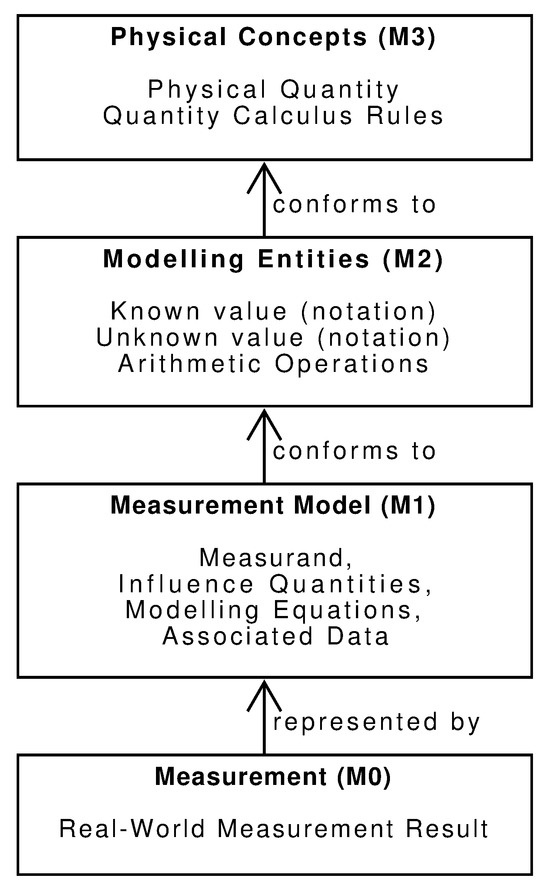
Figure 3.
The four-level hierarchy applied to measurement modelling. A model at level M1 represents the outcome of a measurement in the real world (M0). The elements and rules for constructing this model are defined in the meta-model at level M2. At the top level (M3), fundamental concepts rooted in basic scientific principles form the foundation for all levels. Each M1 model represents a measurement result at M0, conforms to the meta-model at defined M2, and aligns with the high-level concepts established at M3.
Models constructed at the M1 level provide concrete representations of specific measurements. Our focus is on the processes that generate a traceable result. This can be viewed as a sequence of stages, each involving definite quantities that collectively determine the final outcome. Factors such as aleatory behaviour and time dependence of quantities are not relevant.
M1 models represent specific aspects of measurement results to enable reasoning about their properties, such as traceability. In some cases, M1 models may impose additional domain-specific constraints not defined in the M2 meta-model. For example, while quantity calculus allows for the addition of quantities, intensive quantities like temperature cannot be meaningfully added.
5.2. Parallel Hierarchies
Parallel model hierarchies can be developed, extending from the same foundational M3 model, but defining different software entities at the M2 level. Programs at the M1 level, built on these M2 definitions, may serve as models representing different aspects of real-world measurement results.
For instance, distinct M2-level meta-models could support the two types of uncertainty calculation discussed in Section 4.2 and Section 4.3 (Figure 4). A meta-model tailored for GUM uncertainty calculations would define the data type for unknown quantities with attributes such as a value, standard uncertainty, and degrees of freedom. Conversely, a meta-model for MCM calculations would represent unknown quantities with attributes for a value, the state-of-knowledge distribution type, and its associated parameters. The GUM meta-model would also describe how uncertainty is propagated and evaluated using the LPU (A14) and Welch–Satterthwaite (A15) formulae. In contrast, the MCM meta-model would define control structures for Monte Carlo simulations and methods for summarising results. M2 meta-models would also identify the notion of probability applicable to M1 models.
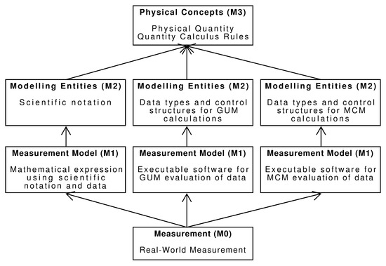
Figure 4.
Three parallel branches of measurement modelling: one using scientific notation, one employing software designed for GUM uncertainty evaluations, and one using software tailored to MCM uncertainty calculations. Each branch originates from the same conceptual basis and addresses the same measurement result in the real-world. While models at a given level are not necessarily directly equivalent between branches, their derivation from shared concepts ensures that logical transformation between models is possible.
5.3. Can the MDA Approach Help in Metrology?
The MDA approach can support the digitalisation of metrology by facilitating a clear separation of concerns. The methodology allows metrologists to focus on describing their problems using metrological principles in scientific terms, while information technologists can concentrate on the design and implementation of robust digital systems. This helps to maintain metrological understanding and scientific integrity throughout the digitalisation process, without placing unnecessary cross-disciplinary demands on either metrologists or IT developers. It also insulates the new digital metrology infrastructure from problems associated with rapid evolution of digital technologies. Flater has expressed similar ideas, observing that the conceptual foundations of a documentary standard often evolve at a different pace than the technologies used in its implementation—a challenge that MDA principles could help address [31].
The key feature of the MDA approach that enables this separation of concerns is its establishment of a common conceptual foundation. This paper illustrated the approach using simple physical modelling applied to measurement results. This conceptual foundation is actually quite effective. Being grounded in fundamental scientific concepts, such as quantities, quantity calculus, and probability, it captures the essential elements required for modelling. Its simplicity is a strength, facilitating clear and unambiguous communication of ideas while offering the flexibility to develop more complex meta-models tailored to specific applications.
Early efforts in the digitalisation of metrology did not exploit hierarchical modelling. Instead, developers created a variety of digital systems where the conceptual foundations were implied rather than explicitly defined. This reliance on a tacit understanding of underlying concepts introduces a risk of ambiguity and inconsistency, particularly when different groups of people or systems interact.
By adopting the MDA approach, however, the metrology community can identify and apply appropriate and well-defined conceptual foundations. This clarity will foster consistency and collaboration between disciplines, reducing misunderstandings and facilitating the creation of more interoperable systems.
6. Discussion
Another perspective on the central theme of this paper is that all measured values are inherently wrong; they inevitably contain some degree of error. Metrologically traceable measurements, however, provide an objective means to quantify the magnitude of that error, enabling the accuracy of measurement to be evaluated so that the usefulness of a result can be considered. Ehrlich and Rasberry suggested that the primary use of traceability was to answer the questions ([14], Section 1.1):
These questions apply between adjacent stages in a traceability chain, where the correction required is the (unknown) value of residual error contributed by the latest stage. However, by iteratively asking these questions back along a traceability chain, we see that the idea aligns with our simple generic model (1)What correction should be applied to a measurement result […] to match the result that would be obtained using the instrument (standard) to which traceability is desired? What is the uncertainty of this corrected result?
The use of “uncertainty” in the VIM definition of traceability serves a pragmatic purpose. Metrologists are accustomed to evaluating the accuracy of measurements in their specialist fields, using methods described in the GUM or its supplements. The results of these evaluations can be reported in a few different formats described in the GUM. Thus, the VIM guides people to use familiar processes that harmonise the way in which information is shared.
Nevertheless, the concept of residual measurement error is central to the scientific understanding of traceability. It is the unknown amount of residual error that leads to uncertainty in the accuracy of a result as an estimate of the measurand. Residual measurement errors can be modelled as instances of physical quantities, representing small deviations from nominal or estimated quantity values. Consequently, measurement models with terms representing errors can be analysed as physical systems. The same cannot be said about uncertainties. In metrology, “uncertainty” broadly refers both to probabilistic descriptions of terms in measurement models (e.g., standard uncertainty) and to the evaluation of statistical inferences about quantity values (e.g., expanded uncertainty) [18]. The sense of “uncertainty” is also complicated by the various interpretations of probability employed within the metrological community.
We contend that measurement models—describing the behaviour of residual errors in traceability chains—provide a framework for understanding the scientific nature of metrological traceability. Such modelling enables a rigorous analysis of measurement scenarios, while the notation avoids some of the challenges inherent in verbal descriptions. The formal language of science, grounded in the strict logic of physical quantity equations, is well suited to this purpose.
There is ample evidence of practical applications to support this contention. The most striking example comes from the microwave metrology community, which has adopted a modelling approach to describe measurements of complex-valued transmission line components. Modelling is described in a best-practice guide for the community [32] and has significantly enhanced the information available through traceable measurements [33]. Modelling, supported by software, can unravel complicated effects due to common influence quantities involved in instrument calibration procedures. Information about the uncertainty components due to residual errors at each stage can be passed between stages along the traceability chain in digital form. This enables downstream users to benefit from the detailed modelling done by an NMI [34].
Another example is a detailed study modelling a four-axis goniometric system measuring optical reflectance [35,36]. This system has many configuration terms that are not known exactly. Residual errors in the estimates of these parameters must be considered to account for the accuracy of the result. By modelling the set-up, the system performance in different configurations could be examined, enabling a better understanding of the correlations between various measurement errors. This understanding significantly improved the accuracy obtainable for certain measurements.
One more example relates to modelling in a recent international CIPM key comparison of the triple point of water (TPW), CCT-K7.2021 [37]. The Measurement Standards Laboratory of New Zealand (MSL) participated in this comparison and used modelling and specialised software to account for significant correlations arising from shared influence factors. MSL submitted an uncertainty in the TPW difference between its comparison artefact and the New Zealand national reference that was less than half the uncertainties submitted by nearly all other participants. While it is unlikely that MSL can measure better than other participants, the uncertainty analysis is complex. The measurement model gives rise to correlations between terms that make rigorous uncertainty analysis by analytical methods difficult; however, these effects can easily be evaluated through automation. After the results of the comparison were published, MSL applied the modelling approach to information reported by the pilot laboratory. A mathematical model for the pilot laboratory’s measurement was derived from the written description in the report, and this model was evaluated using the published data. The result was a 2.5-fold reduction in the pilot laboratory’s uncertainty [38].
A common feature of these examples is the use of specialised software that implicitly adopts a modelling approach similar to the one discussed in this article. Several NMIs have developed such packages [39,40], highlighting the benefits of adopting a clear semantic structure, in line with the MDA principles discussed in Section 5.2. However, the overarching conceptual model is embedded within the uncertainty evaluation algorithm, rather than being explicitly specified. These software tools define an abstract data type to represent unknown quantities in a measurement model [41]. Objects of this type possess the attributes needed for GUM-based uncertainty evaluation (Appendix B). In this way, much of the computational complexity can be automated. Ideally, however, the definition of measurement models should be decoupled from the software responsible for uncertainty evaluation, as outlined in Section 5.2.
7. Conclusions
The most important aspect of metrological traceability is that results can be meaningfully compared—whether with other traceable results or with nominal values expressed on the same measurement scale. To enable this, measurement results include a quantitative assessment of accuracy. Accuracy is determined by the inevitable accumulation of residual errors during measuring stages, so a measurement model that describes how these errors contribute to the final result is essential.
This paper presented a structured approach to modelling using a simple mathematical notation. A number of examples were presented that showed how to develop models using this framework. We emphasised the importance of modelling the entire traceability chain, from the realisation of primary reference standards through to the end user. This ensures that all residual errors can be properly accounted for in the accuracy assessment of a final result, wherever they arose during measuring processes. We also emphasised the need for a static model of the quantities involved. A static model consists of terms representing definite values of quantities contributing to the final result—like a snapshot of the physical situation.
The modelling approach described here is grounded in physical principles, including the concepts of physical quantities and quantity calculus. Modelling does not involve notions of probability or measurement uncertainty; however, a model serves as a precursor to uncertainty calculations. Whether the original GUM method or the GUM Supplement’s Monte Carlo Method is used, an evaluation of uncertainty requires a static model of the measurement as a starting point. Static modelling of the entire chain has the advantage of eliminating the need to explicitly distinguish between random and systematic errors, as both are inherently accounted for within the model.
The importance of clearly identifying a formal semantic basis for modelling was discussed in relation to modern methods of digital system design. We argue that creating hierarchical modelling structures, anchored in well-defined conceptual models, holds promise for the further development of digitalisation in metrology. Doing so cleanly separates the concerns of metrology from others related to computation and technology, both during the development of new digital systems and their subsequent maintenance. This is well suited to a formal, structured, enterprise-based approach to architectural planning of digital transformation in metrology. Logical next steps for the ideas discussed above will be to formalise the model notation details, allowing it to be incorporated in standardised architectural descriptions. This could be achieved by following established standards for documenting architectural descriptions, like the ISO/IEC standard 42010 [42].
Funding
This work was funded by the New Zealand government.
Data Availability Statement
No new data were created or analysed in this study. Data sharing is not applicable to this article.
Acknowledgments
The author is grateful to Ellie Molloy and Peter Saunders for carefully reviewing this work, and to Rod White for suggestions relating to the preprint version.
Conflicts of Interest
The author declares no conflicts of interest.
Abbreviations
The following abbreviations are used:
| CIPM | International Committee for Weights and Measures |
| CGPM | General Conference on Weights and Measures |
| ILAC | International Laboratory Accreditation Cooperation |
| GUM | Guide to the Expression of Uncertainty in Measurement |
| VIM | International Vocabulary of Metrology |
| ISO | International Organisation for Standardization |
| MRA | Mutual Recognition Agreement |
| NMI | National Metrology Institute |
| NIST | National Institute of Standards and Technology |
| QI | Quality Infrastructure |
Appendix A. Calibrating a Linear Measuring System
The observation equation of a simple system for measuring a quantity Q is
The system produces an indication for each measurement. Its response is characterised by a gain, G, and an offset, O, both of which must be determined to calibrate the system. Additionally, measured values exhibit variability, which is modelled by a term for each indication.
A minimum of two calibration standards are needed to measure G and O. We assume that standards for and are available, where the residual errors and represent the fact that and are not known exactly. The system responses to the calibration standards are
Solving for the gain and offset, we obtain
The measurement model of the system is
The explicit influence of factors involved in the calibration can be seen by substituting for G, O, , and and rearranging terms
It is not uncommon for one of the calibration standards to represent the absence of Q (e.g., ), corresponding to a nominal value of zero, and another to represent a nominal value of unity (e.g., ). However, this does not significantly simplify the model (A9), as it does not remove any of the influence terms.
Appendix A.1. Difference Measurement
If the system is used to measure , the offset term cancels. However, the approximate values attributed to calibration standards continue to influence the measurement:
Appendix A.2. Ratio Measurement
If the system is used to measure , the gain term cancels out in the measurement model. However, the offset remains as an influence factor and is correlated with the gain measurement during calibration
By incorporating more detailed expressions for G, , and , Equation (A12) can be expanded to reveal specific residual errors associated with calibration, as in Equation (A10).
Appendix B. GUM Evaluation of Uncertainty—Summary
The GUM describes a method for evaluating measurement uncertainty based on a function of the form given in (22):
where the output quantity Y is the measurand, and are input quantities on which Y depends. A measured value, y, for Y, is obtained by evaluating using the best estimates available for each of the input quantities, .
The method of evaluating the uncertainty is known as the Law of Propagation of Uncertainty (LPU) ([16], clause 5). To evaluate the uncertainty of y as an estimate of Y, the following information about input estimates is needed:
- Each input estimate has a standard uncertainty, denoted ;
- Each standard uncertainty has a number of degrees of freedom, denoted ;
- A correlation coefficient, , must be provided if input estimates are correlated.
The LPU considers components of uncertainty, which are defined in terms of the sensitivity of Y to changes in a particular input. The component of uncertainty for is
The LPU evaluates the combined standard uncertainty of y as
where when , and in the absence of correlation. There is also an expression called the Welch–Satterthwaite formula to evaluate , the effective degrees of freedom of ([16], clause G.4),
Thus, the estimate y of Y is associated with a standard uncertainty that has a number of degrees of freedom, just like the data available for input quantity estimates.
We take the view that Equation (22) should describe the whole traceability chain, which raises the question: can the LPU still be implemented if calculations are performed at each stage and the results are passed from stage to stage? The answer is yes [43]. The evaluation of Equations (A14) and (A15) is only required at the end of the chain. However, to enable this, a set of uncertainty components must be determined at each stage, along with the corresponding measured value. Thus, the intermediate results propagated from one stage to the next should consist of the stage value, , and the set of components of uncertainty in for all inputs. These components of uncertainty are of the form
Appendix C. The Monte Carlo Method of Uncertainty Evaluation—Summary
The first supplement to the GUM describes a Monte Carlo Method (MCM) for evaluating measurement uncertainty ([26], clause 5.9). The approach also applies to a function of the form given in (22):
where the output quantity Y is the measurand, and are input quantities on which Y depends. The second supplement to the GUM, which addresses the evaluation of uncertainty in multivariate quantities, describes the extension of the MCM to multivariate measurands ([27], clause 7).
To evaluate the uncertainty of y as an estimate of Y, a joint probability density function for the input quantities to Equation (22) must be determined ([27], clause 6). This task is potentially challenging; however, in practice, a selection of common state-of-knowledge distributions is available to choose from ([26], Table 1).
The MCM implements an approximate form of propagation of distributions. It samples from random deviates generated by probability distributions associated with the input quantities. Repeating this many times accumulates a set of values, which is characteristic of the probability distribution function, , for the output Y. The MCM data set can be used to evaluate the expectation and suitable quantile information for that can be reported as a measured value and its uncertainty, respectively.
Our view is that Equation (22) should describe the full traceability chain, which raises the following question: can the MCM still be implemented if calculations are performed at each stage and the results are passed from stage to stage? It is more difficult to give a clear answer to this question than it was for the LPU calculation in Appendix B. Often, it is sufficient to pass the MCM data set, evaluated for at the kth stage, to the next stage. However, when the traceability chain has a branching structure that is not a simple tree, common influence factors may become important. If MCM data for a common influence must be accessed at several stages, it complicates the information-passing requirements between stages.
References
- BIPM; OIML; ILAC; ISO. Joint BIPM, OIML, ILAC, and ISO Declaration on Metrological Traceability. 2011. Available online: https://www.bipm.org/documents/20126/42177518/BIPM-OIML-ILAC-ISO_joint_declaration_2011.pdf (accessed on 11 April 2025).
- CIPM. Mutual Recognition of National Measurement Standards and of Calibration and Measurement Certificates Issued by National Metrology Institutes. 1999. Available online: https://www.bipm.org/documents/20126/43742162/CIPM-MRA-2003.pdf (accessed on 17 April 2023).
- ILAC. ILAC Mutual Recognition Arrangement: Scope and Obligations. 2022. Available online: https://ilac.org/publications-and-resources/ilac-policy-series/ (accessed on 17 April 2023).
- Rasberry, S.D.; Belanger, B.; Garner, E.; Brickencamp, C.; Ehrlich, C.D. Traceability: An Evolving Concept. In A Century of Excellence in Measurements, Standards, and Technology; National Institute of Standards and Technology: Gaithersburg, MD, USA, 2001; Volume SP 958, pp. 167–171. [Google Scholar]
- Belanger, B.C. Traceability: An evolving concept. ASTM Stand. News 1980, 8, 22–28. [Google Scholar]
- Belanger, B.C. Traceability in the USA: An evolving concept. Bull. OIML 1980, 78, 12–25. Available online: https://www.oiml.org/en/publications/bulletin/pdf/1980-bulletin-78.pdf (accessed on 11 April 2025).
- Nicholas, J.V.; White, D.R. Traceable Temperatures: An Introductory Guide to Temperature Measurement and Calibration; Science Information Division, DSIR: Wellington, New Zealand, 1982. [Google Scholar]
- BIPM; IEC; ISO; OIML. Vocabulary of Metrology, Part 1, Basic and General Terms (International), 1st ed.; ISO: Geneva, Switzerland, 1984. [Google Scholar]
- BIPM; IEC; IFCC; IUPAC; IUPAP; ISO; OIML. International Vocabulary of Basic and General Terms in Metrology, 2nd ed.; ISO: Geneva, Switzerland, 1993. [Google Scholar]
- BIPM; IEC; IFCC; ISO; IUPAC; IUPAP; OIML. Guide to the Expression of Uncertainty in Measurement, 1st ed.; ISO: Switzerland, Geneva, 1993. [Google Scholar]
- BIPM; IEC; IFCC; ILAC; IUPAC; IUPAP; ISO; OIML. International Vocabulary of Metrology—Basic and General Concepts and Associated Terms (VIM), 3rd ed.; BIPM Joint Committee for Guides in Metrology: Paris, France, 2012. [Google Scholar]
- De Bievre, P. Metrological traceability is a prerequisite for evaluation of measurement uncertainty. Accredit. Qual. Assur. 2010, 15, 437–438. [Google Scholar] [CrossRef]
- De Bievre, P. Making measurement results metrologically traceable to SI units requires more than just expressing them in SI units. Accredit. Qual. Assur. 2010, 15, 267–268. [Google Scholar] [CrossRef]
- Ehrlich, C.D.; Rasberry, S.D. Metrological timelines in traceability. J. Res. Natl. Inst. Stand. Technol. 1998, 103, 93. [Google Scholar] [CrossRef] [PubMed]
- Cox, M.G.; Harris, P.M. Measurement uncertainty and traceability. Meas. Sci. Technol. 2006, 17, 533. [Google Scholar] [CrossRef]
- BIPM; IEC; IFCC; ISO; IUPAC; IUPAP; OIML. Evaluation of Measurement Data—Guide to the Expression of Uncertainty in Measurement JCGM 100:2008 (GUM 1995 with minor Corrections), 1st ed.; BIPM Joint Committee for Guides in Metrology: Paris, France, 2008. [Google Scholar]
- CGPM. Resolution 2—On the Global Digital Transformation and the International System of Units. 2022. Available online: https://www.bipm.org/en/cgpm-2022/resolution-2 (accessed on 17 April 2023).
- White, D.R.; Hall, B.D.; Saunders, P. The purposes of measurement uncertainty. AIP Conf. Proc. 2024, 3220, 150001. [Google Scholar] [CrossRef]
- Willink, R. A formulation of the law of propagation of uncertainty to facilitate the treatment of shared influences. Metrologia 2009, 46, 145–153. [Google Scholar] [CrossRef]
- CIPM. Measurement Comparisons in the CIPM MRA; Technical Report; Bureau International des Poids et Mesures: Pavillon de Breteuil, France, 2021; Version 1.0. [Google Scholar]
- Koo, A.; Hall, B.D. Linking an RMO or Bilateral Comparison to a Primary CCPR Comparison; Technical Report 0776; Callaghan Innovation: Lower Hutt, New Zealand, 2020. [Google Scholar] [CrossRef]
- Hall, B.D.; Koo, A. Digital Representation of Measurement Uncertainty: A Case Study Linking an RMO Key Comparison with a CIPM Key Comparison. Metrology 2021, 1, 166–181. [Google Scholar] [CrossRef]
- Wallard, A.J.; Quinn, T.J. “Intrinsic” standards—Are they really what they claim? Cal Lab Int. J. Metrol. 1999, 6, 28–30. [Google Scholar]
- Pettit, R.; Jaeger, K.; Ehrlich, C. Issues in Purchasing and Maintaining Intrinsic Standards. Cal Lab Int. J. Metrol. 2000. Available online: https://www.osti.gov/biblio/762126 (accessed on 26 April 2025).
- Hall, B.D. An Opportunity to Enhance the Value of Metrological Traceability in Digital Systems. In Proceedings of the 2019 IEEE International Workshop on Metrology for Industry 4.0 and IoT (MetroInd4.0&IoT), Naples, Italy, 4–6 June 2019; IEEE: Piscataway, NJ, USA, 2019; pp. 16–21. [Google Scholar] [CrossRef]
- BIPM; IEC; IFCC; ISO; IUPAC; IUPAP; OIML. Evaluation of Measurement Data—Supplement 1 to the “Guide to the Expression of Uncertainty in Measurement”—Propagation of Distributions Using a Monte Carlo Method JCGM 101:2008, 1st ed.; BIPM Joint Committee for Guides in Metrology: Paris, France, 2008. [Google Scholar] [CrossRef]
- BIPM; IEC; IFCC; ISO; IUPAC; IUPAP; OIML. Evaluation of Measurement Data—Supplement 2 to the “Guide to the Expression of Uncertainty in Measurement”—Extension to Any Number of Output Quantities JCGM 102:2011, 1st ed.; BIPM Joint Committee for Guides in Metrology: Paris, France, 2011. [Google Scholar] [CrossRef]
- Hebner, R.E. Calibration Traceability: A Summary of NIST’s View, 1996.
- Group, O.M. Model Driven Architecture (MDA). 2003. Available online: https://www.omg.org/mda/ (accessed on 17 January 2025).
- Bézivin, J. On the Unification Power of Models. Softw. Syst. Model. 2005, 4, 171–188. [Google Scholar] [CrossRef]
- Flater, D. Impact of model-driven standards. In Proceedings of the 35th Annual Hawaii International Conference on System Sciences, Big Island, HI, USA, 7–10 January 2002; pp. 3706–3714. [Google Scholar] [CrossRef]
- Zeier, M.; Allal, D.; Judaschke, R. Guidelines on the Evaluation of Vector Network Analysers (VNA), 3rd ed.; EURAMET Calibration Guide; EURAMET: Braunschweig, Germany, 2018; Volume cg-12, Available online: https://www.euramet.org/publicationsmedia-centre/calibration-guidelines/ (accessed on 11 April 2025).
- Wollensack, M.; Hoffmann, J.; Ruefenacht, J.; Zeier, M. VNA Tools II: S-parameter uncertainty calculation. In Proceedings of the ARFTG Microwave Measurement Conference Digest, Montreal, QC, Canada, 22 June 2012; Volume 79. [Google Scholar] [CrossRef]
- Zeier, M.; Rüfenacht, J.; Wollensack, M. VNA Tools—A software for metrology and industry. In METinfo; Federal Institute of Metrology META: Wabern, Switzerland, 2020; Volume 27/2, pp. 4–6. [Google Scholar]
- Molloy, E.; Saunders, P.; Koo, A. Effects of rotation errors on goniometric measurements. Metrologia 2022, 59, 025002. [Google Scholar] [CrossRef]
- Molloy, E. Metrology of Scattering Distributions. Ph.D. Thesis, Te Herenga Waka-Victoria University of Wellington, Wellington, New Zealand, 2023. Available online: https://openaccess.wgtn.ac.nz/articles/thesis/Metrology_of_Scattering_Distributions/23735001 (accessed on 26 April 2025).
- Peruzzi, A.; Dedyulin, S.; Levesque, M.; Campo, D.d.; Izquierdo, B.G.; Gomez, M.; Quelhas, K.; Neto, M.; Lozano, B.; Eusebio, L.; et al. CCT-K7.2021: CIPM key comparison of water-triple-point cells. Metrologia 2023, 60, 03002. [Google Scholar] [CrossRef]
- Molloy, E.; Saunders, P. Uncertainty Analysis of MSL’s CCT-K7. 2021 Key Comparison Measurements Taking Account of Correlations. Metrologia 2025. submitted. [Google Scholar]
- Zeier, M.; Wollensack, M.; Hoffmann, J. METAS UncLib—A measurement uncertainty calculator for advanced problems. Metrologia 2012, 49, 809–815. [Google Scholar] [CrossRef]
- Hall, B.D. The GUM tree calculator: A python package for measurement modelling and data processing with automatic evaluation of uncertainty. Metrology 2022, 2, 128–149. [Google Scholar] [CrossRef]
- Hall, B.D. Computing with Uncertain Numbers. Metrologia 2006, 43, L56–L61. [Google Scholar] [CrossRef]
- ISO; IEC; IEEE. Systems and Software Engineering—Architecture Description, 2nd ed.; International Standards Organisation: Geneva, Switzerland, 2022. [Google Scholar]
- Hall, B.D. Propagating uncertainty in instrumentation systems. IEEE Trans. Instrum. Meas. 2005, 54, 2376–2380. [Google Scholar] [CrossRef]

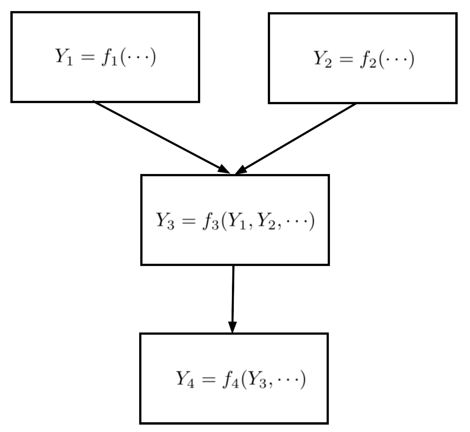

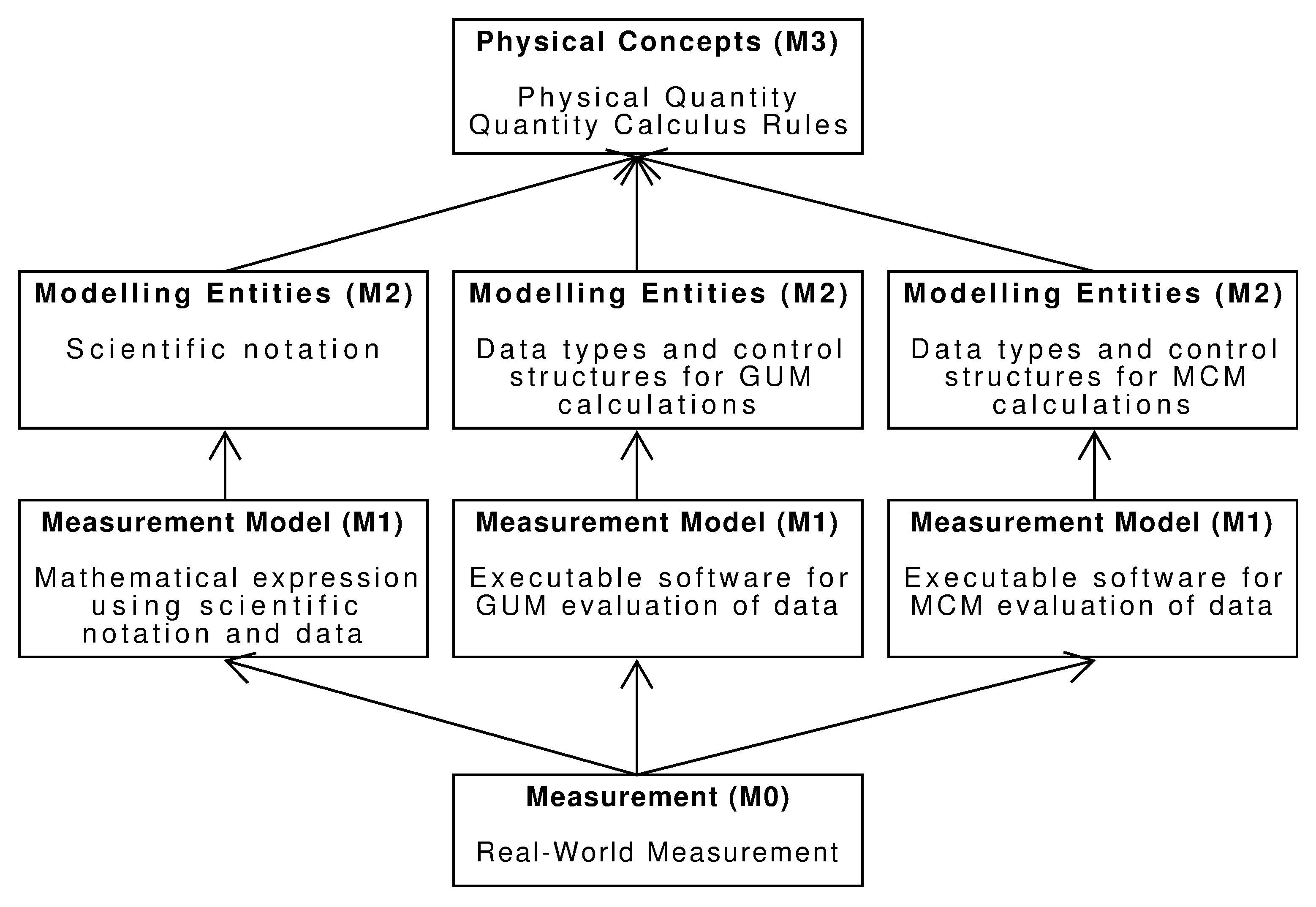
Disclaimer/Publisher’s Note: The statements, opinions and data contained in all publications are solely those of the individual author(s) and contributor(s) and not of MDPI and/or the editor(s). MDPI and/or the editor(s) disclaim responsibility for any injury to people or property resulting from any ideas, methods, instructions or products referred to in the content. |
© 2025 by the author. Licensee MDPI, Basel, Switzerland. This article is an open access article distributed under the terms and conditions of the Creative Commons Attribution (CC BY) license (https://creativecommons.org/licenses/by/4.0/).