Spatial Patterns in Fibrous Materials: A Metrological Framework for Pores and Junctions

Abstract

Several materials widely used in scientific research and industrial applications, including nano-filters and neuromorphic circuits, consist of fiber structures. Despite the fundamental structural similarity, the key feature that should be considered depends on the specific application. In the case of membranes and filters, the main concern has been on the pores among fibers, whereas in neuromorphic networks the main functionality is performed through the junctions of nanowires simulating neuron synapses for information dissemination. Precise metrological characterization of these structural features, along with methods for their effective control and replication, is essential for optimizing performance across various applications. This paper presents a comprehensive metrological framework for characterizing the spatial point patterns formed by pores or junctions within fibrous materials. The aim is to probe the influence of fiber randomness on both the point patterns of intersections (ppi) and pores (ppp). Our findings indicate a strong tendency of ppi toward aggregation, contrasting with a tendency of ppp toward periodicity and consequent pore uniformity. Both patterns are characterized by peculiarities related to collinearity effects on neighboring points that cannot be captured by the conventional anisotropy analysis of point patterns. To characterize local collinearity, we develop a method that counts the number of collinear triplets of nearest neighbor points in a pattern and designs an appropriate parameter to quantify them, also applied to scanning electron microscopy (SEM) images of membranes, demonstrating consistency with simulated data.

1. Introduction

Fibrous materials have found extensive applications [1,2] in science and industry due to their unique mechanical, thermal, and optical properties. In the biomedical field [3,4], fibrous materials, mainly composed of electrospun hybrid polymer nanofibers, are utilized as scaffolds for tissue engineering and wound healing. They also serve as filters [5], separators [6], and carriers [7] in various biotechnological processes. In the energy sector, fibrous materials are utilized as insulation [8] materials, battery separators [9], and heat exchangers [10]. Furthermore, fibrous materials are used in a range of consumer products, including textiles [11], paper [12], and hygiene products, notably for water purification processes [13]. Their widespread use is attributed to the availability of various methods for their synthesis and processing, with electrospinning [14] being the most prominent, which allow for the development of materials with tailored properties to meet specific applications. Additionally, quite recently, the advent of nanowire networks formed by randomly distributed metal nanowires on a surface [15,16,17,18] has followed the rise of neuromorphic computing. Their apparent randomness gives their network circuitry a complicated topology and embeds a higher interconnectivity of resistive switching memory (memristive) cross-point junctions. The functional performance of fibrous materials is closely tied to their structural and geometrical attributes, particularly the spatial arrangement of fibers. Metrological studies of these structures provide a quantitative understanding essential for tailoring materials to these specific applications.

Despite the different fields of applications, nanowire networks and fibrous structures share similar geometrical properties. Both consist of fibers that are interwoven in a complicated random-like manner to form a 2D or 3D layer. In the case of membrane fiber networks, the fibers are usually curved lines whose curvature depends on their material properties and fabrication process. On the other side, the nanowires in neuromorphic networks are short straight-line segments with variable length and orientation. Furthermore, in membranes, the key feature for their performance are the pores [12] formed in the spaces/voids between fibers, whereas in neuromorphic networks, the focus has mainly been on the nanowire junctions comprising the circuit memristive elements [18]. Although we consider infinite straight-line segments, this simulation serves as a decent approximation for fiber network structure. This approximation applies to many non-woven materials, where the fiber extension is much longer than local correlations. As for electrospun networks, where the fiber is created as a continuous filament, we anticipate strong agreement in the simulation for these materials as well.

In both cases one can recognize the critical role of the formatted point patterns, i.e., the pore centers in fibrous materials and the nanowire intersections in neuromorphic networks. More analytically [15,16,17,18], in the case of intersections, this point pattern is paramount for advancing the efficiency and functionality of neuromorphic systems. These networks, designed to emulate the intricate architecture of biological neural networks, rely on high-density connectivity to accurately replicate neural processes. The arrangement of intersections directly influences signal routing efficiency, minimizing crosstalk and ensuring clear signal transmission. An optimized intersection pattern reduces power consumption by minimizing interconnection lengths and complexities, enhancing the system’s energy efficiency. Additionally, it contributes to the network’s fault tolerance and robustness, providing multiple pathways for signal transmission and ensuring operational continuity despite potential connection failures. Therefore, understanding and optimizing the point pattern of intersections is essential for developing scalable, efficient, and robust neuromorphic networks that can more effectively replicate the complex functionalities of biological neural systems.

As for the study of the pore centroids pore pattern, in the development of carbon-based materials for supercapacitors, precise control over pore size and distribution is essential to balance surface area, density, and conductivity, which are often mutually exclusive properties [19]. Additionally, in biomedical engineering, the arrangement of pores significantly influences mechanical properties and permeability, with topology optimization approaches used to tailor these properties for specific needs [20]. For porous media, the spatial distribution of permeabilities and porosities directly impacts fluid transport properties, highlighting the necessity of detailed pore pattern analysis [21]. Thus, a comprehensive understanding of pore centroid patterns is vital for the design and optimization of materials across diverse scientific and engineering fields.

Despite their critical importance, the geometrical and stochastic properties of these point patterns have not been extensively studied. Key metrological challenges arise in analyzing these point patterns, particularly the distribution of pore centroids in fibrous materials and junctions in nanowire networks. Accurate quantification of these spatial point patterns is essential for advancing material functionality. The ability to measure these patterns is critical for optimizing the structural attributes of materials.

This study addresses these metrological needs by employing advanced methods in stochastic geometry. Building upon established techniques for modeling fibrous materials and line processes, we propose a framework to quantify the spatial arrangement of pores and junctions. The application of stochastic mathematical models to describe the structure [22,23] of the types of fibrous networks seems crucial in the understanding of their properties. Sampson’s work [24] on their modelling and spatial variability is of high importance for the field, along with Eichhorn’s [25] fibrous materials statistical geometry approach. Miles [26] and Abdel-Ghani [27] laid strong mathematical foundations for the field, constituting seminal works. Dodson [28] later demonstrated via simulations that there is a correlation between the lengths of adjacent sides of polygons created in the plane by the crossings of random line processes. More notably, Chiu, Stoyan, Kendall, and Mecke’s book on Spatial Statistics [29] compacted a plethora of theoretical results available for Poisson line processes and Poisson line tessellations, while also Barthélemy [30] approached line processes and tessellations with mostly network metrics.

In this work, we focus on metrics inspired by Point Pattern Analysis (PPA) [31] to quantify the spatial pattern properties of these complex point structures. The spatial point processes developed in PPA are mathematical models describing the arrangement of objects that are irregularly or randomly distributed on a plane. In our case, the point patterns are extracted by lines/fibers on a plane enclosed in a square inspection area (Figure 1b). Various methodologies can be employed in the construction of random lines on a two-dimensional plane. In this work, we apply the I randomness methodology [27]: the line creation process involves the random selection of a point within the square and the random determination of a slope value with respect to the horizontal axis. The coordinates of the initial point and the slope are chosen from independent white noise distributions.

We focus on two types of pp: the pp of the intersections (junctions) of the fibers (ppi), and the point pattern of the centroids of the pores (ppp), as showcased in Figure 1c and Figure 1d, respectively. The pore structure of a fibrous material is formed by the void space created by the distribution of the fibers. As such, it is understandable that the spatial structure of the points in these pp is influenced by the fiber arrangement. This study analyzes both simulated and experimental fiber structures. The experimental dataset consists of SEM (Scanning Electron Microscopy) images from nanofilament coated PES (Polyethersulfone) membranes [32], as showcased in Figure 1a.

Due to the linear nature of fibers, special emphasis will be given on the anisotropy [33,34] of the emerged point patterns. In particular, inspired by the different kinds of anisotropy detected in the pp of such networks, we propose a method to analyze and characterize the local anisotropy of the obtained point patterns (ppi and ppp) based on the collinearity these patterns exhibit (LocalColLinearity method—LCL).

The paper is set out in the following way to achieve the aforementioned objectives. In Section 2, the methodologies for the analysis of both point pattern randomness and anisotropy (global and local) are described in detail. Section 3 presents the results of our study divided in subsections for the point patterns of simulated and experimental cases respectively. Special attention is paid to the novel metric of local collinearity quantifying local anisotropy. The paper closes with an enumeration of the conclusions in Section 4, along with some future work suggestions.

2. Materials and Methods

2.1. Methods

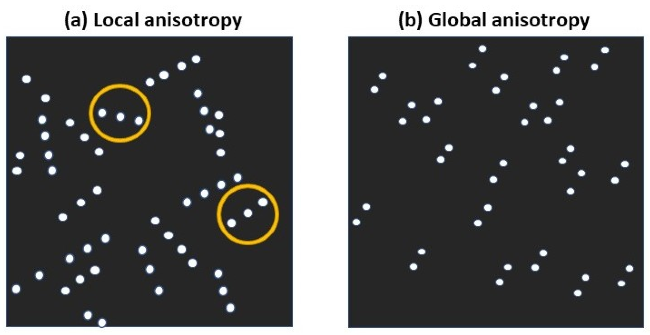
2.1.1. Global and Local Anisotropy

Anisotropy measures are frequently discussed in the literature [34]. To name some of the widely used and most influential: Fry plots, nearest neighbor analysis, Ripley’s K, pair correlation function, and wavelet analysis. Global anisotropy metrics omit the detection of local directionality phenomena such as those created by collinear nearest neighbor points, which can be heavily observed in the ppi and partially in the ppp. The collinearity of at least a triad of points is a different kind of anisotropy than the conventional above-mentioned methods can detect, since it focuses on each of these triads, thus having an interest in local point interactions and can be considered local anisotropy.

Therefore, traditional nearest neighbor measures are usually not sensitive to the intrinsic properties of aggregates, making local anisotropy an informative method for accurately characterizing the aggregates in such scenarios. This is particularly relevant in our case, where the point patterns of intersections and pore centroids extracted from fiber networks are studied.

By applying local anisotropy, we aim to gain deeper insights into the structural properties and spatial relationships within these networks. This approach allows us to discern subtle differences and intrinsic features that are critical for understanding the underlying mechanisms and properties of the fiber networks that traditional methods may overlook.

Figure 2 visualizes two different point patterns characterized by local and global anisotropy, respectively. In the diagram of Figure 2a, we highlight, with the yellow circle, a triad of collinear points exhibiting local directionality and anisotropy, though the whole point pattern is globally isotropic. On the contrary, the point pattern of Figure 2b does not have triads of collinear points but all the couples of neighbor points have similar orientations. Needless to say, one can find cases where both types of anisotropy (local and global) are mixed together in a single point pattern.

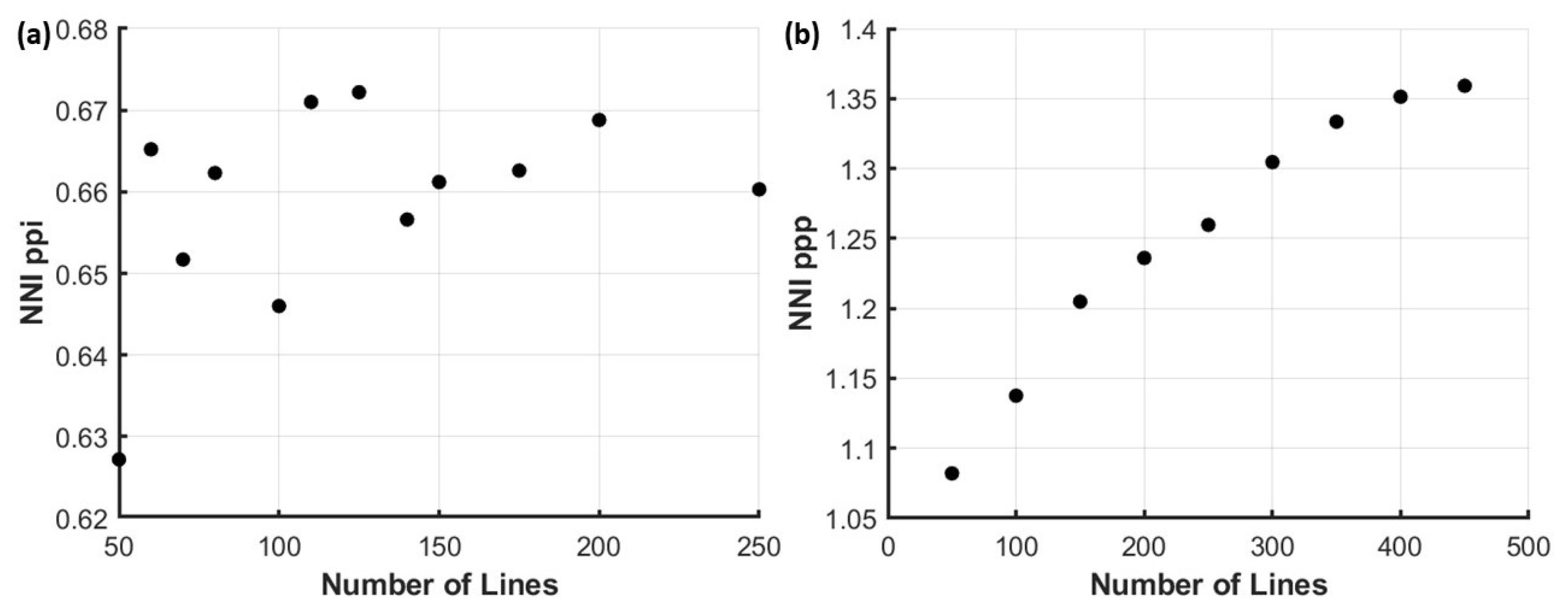
2.1.2. Nearest Neighbor Index (NNI)

A fundamental question in point pattern analysis is the characterization of the degree of randomness of a point pattern. A popular metric used to meet this requirement is the Nearest Neighbor Index (NNI), which is based on the concept of nearest neighbor distances d_i i = 1, …, N, i.e., the distance between the i-th point and its nearest neighbor. In a point pattern consisting of N points on an area A, NNI is defined by the ratio of the average nearest neighbor distance $d_A=<d_i>$ over the expected one d_E under the assumption of complete spatial randomness.

When the hypothesis of complete spatial randomness (CSR) holds, the expected distance $d_E$ is determined as follows: $d_E=0.5\sqrt{A/N}$, because the distribution of the points on area A follows Poisson statistics [31]. Accordingly, the NNI is given by:

$$NNI={\displaystyle \frac{d_A}{d_E}}={\displaystyle \frac{⟨d_i⟩}{0.5\sqrt{\frac{A}{N}}}}$$

(1)

NNI is indicative of the deviation of the observed point pattern from the CSR hypothesis and can quantify the degree of clustering (NNI < 1) or periodicity (NNI > 1 with a maximum value of 2.15 for a strict hexagonal pattern) in the spatial distribution of the points forming the pattern. It should be noted that when NNI values deviate from 1, with a percentage larger than 10%, then the deviation from complete spatial randomness can be considered significant [35,36].

NNI is affected by the area A of the image that represents the point pattern’s finiteness [37]. Bias ought to be considered as a result. This bias is quantified using what are known as edge effects because points close to the border-edges of the image could have a nearest neighbor beyond the region displayed. In these circumstances, corrective methods that calculate the relative importance of each pattern point’s influence are used. The algorithms described in the literature cover a wide range, from methods for pattern extensions to the more popular border and nearest neighbor (or weighted) methods, which consider sections of the image.

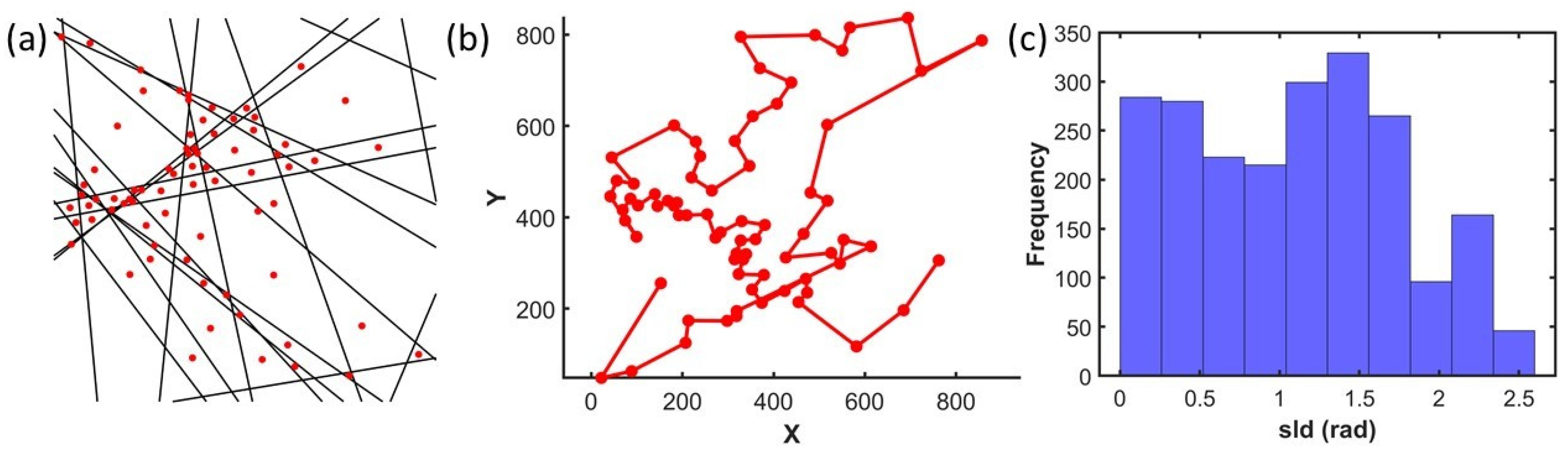
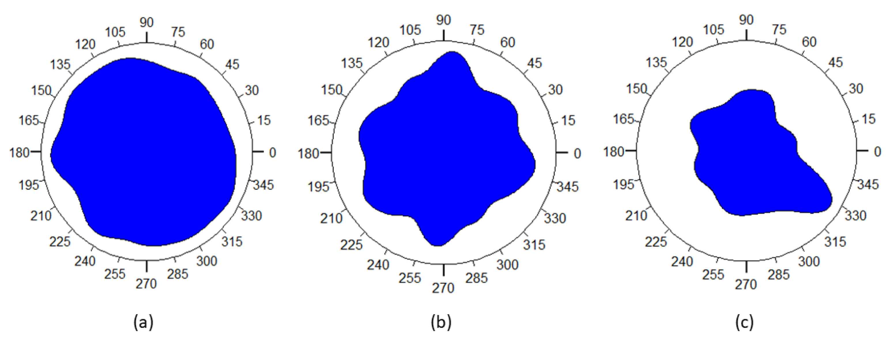
2.1.3. Nearest Neighbor Orientation Distribution

The NNI index is a classic and useful measure of quantifying the randomness in a point pattern, although it is limited to the statistics of nearest neighbor distances, which omits phenomena of directionality. To capture such phenomena, we can consider the distribution of the orientation on the plane of the directed line connecting a point with its nearest neighbor and calculate the nearest neighbor orientation distribution.

The planar case is considered, where the angle $t$ expresses the angle of the line (more accurately of the vector) connecting the point with its nearest neighbor, with respect to the horizontal direction, (i.e., x axis) measured in radians, i.e., $0\le t<2\pi$.

The probability density function $\vartheta \left(t\right)$ is constant for the CSR (Poisson) case:$\vartheta \left(t\right)\equiv {\displaystyle \frac{1}{2\pi }}.$ This $\vartheta \left(t\right)$ metric is statistically estimated utilizing a kernel estimator, and considering the edge effects introduced in Section 2.1.1 with nearest-neighbor edge correction. Accordingly, $\hat{\vartheta }(t)$ is calculated [31]:

$$\hat{\vartheta }(t)={\sum }_{i=1}^n {\displaystyle \frac{1\left(d_i\left(x\right)\le e_i\left(x\right)\right)k\left(t-t_i\right)}{\nu \left(W_{\ominus d_i\left(x\right)}\right)}}/{\hat{\lambda }}_{nn}$$

(2)

where, $t_i$ is the angle of the line connecting the $i$ th point of the pattern to its nearest neighbor point, $k$ is the kernel function with bandwidth $h$, $d_i\left(x\right)$ is the nearest neighbor distance, and $e_i\left(x\right)$ is the lowest distance of the point from the edges of the image.

The indicator ${\hat{\lambda }}_{nn}$ is calculated as:

$${\stackrel{\mathrm{ˆ}}{\mathsf{\lambda }}}_{\mathrm{n}\mathrm{n}}={\sum }_{\mathrm{x}\in \mathrm{W}} 1(d_i(x)\le e_i(x))/\mathsf{\nu }\left({\mathrm{W}}_{\ominus d_i\left(x\right)}\right)$$

(3)

If the window $W$ in which the points exist has sides $a$ and $b$ and is of rectangular shape, the weights are estimated as follows:

$$\nu \left(W_{\ominus d\left(x\right)}\right)=(a-2d(x\left)\right)(b-2d(x\left)\right) \mathrm{for} a>2d\left(x\right)\mathrm{and}b>2d\left(x\right)$$

(4)

where $W_{\ominus d}$ is notation for $W\ominus b(o,r),\mathrm{w}\mathrm{i}\mathrm{t}\mathrm{h} \ominus$ denoting Minkowski subtraction and $b(o,r)$ being the sphere with radius $r$ and centre at $0$.

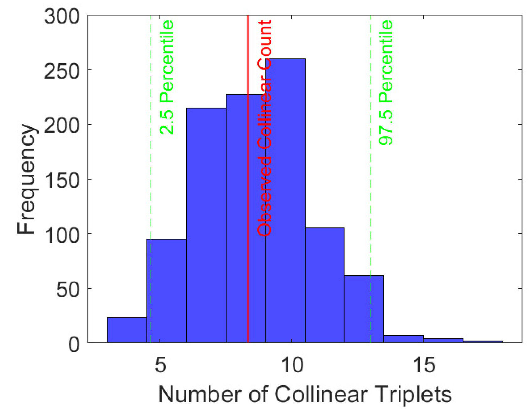
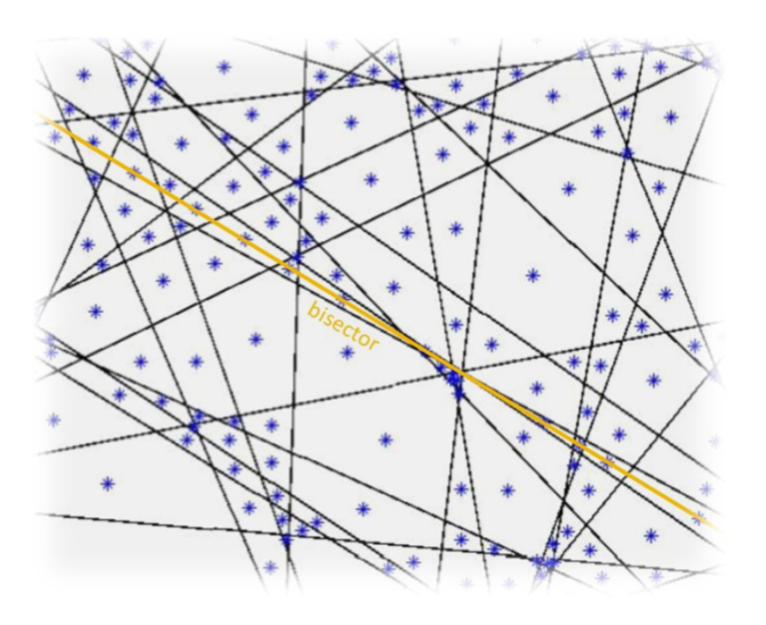
2.1.4. Local Collinearity Characterization (LCL)

To quantify the presence of collinear points in a point pattern (i.e., at least three points on a straight line), we propose a Local Collinearity method (LCL) defined by the following steps: with a given pp, we begin the analysis by randomly choosing one point and connect it with its nearest neighbor. We continue with the nearest neighbor of the new point and so on until all the points are uniquely joined to their nearest neighbor point that has not been connected yet. Thus, a path is created that visually may resemble a random walk, as seen in Figure 3b, where such a path has been drawn for the ppp of the line pattern shown in Figure 3a. It should be emphasized that no loops are allowed due to the unique participation of each point in the walk. A side effect is the appearance of long line segments at the end of path formation, which results from the fact that points may share their nearest neighbor, but due to the conditions of the LCL path, a point may be incorporated in the path only once. We then choose the successive line segments created by the connected points and compare their slopes by calculating their difference:

$$sl{d}_i=\left|s{l}_{i+1}-s{l}_i\right|$$

(5)

where $s{l}_{i+1}$ and $s{l}_i$ are the slopes of the (i + 1)-th and i-th line segments created by the unique connection of the nearest neighbor points with respect to the horizontal axis. Three points will be exactly collinear if the slope difference is 0. Four points create two possible triads, so they will produce two slope differences. Thus, for a pattern of n points, there exist n-2 possible triads. In Figure 3c, the histogram of difference of slope values, which distributes the slopes of all the point triads for the ppp of Figure 3a, is presented. Figure 4 shows an example visualization of three line segments connecting each point to its nearest neighbor. Each segment is noted after its i-th point, and its consecutive segment as the (i + 1)-th point. The notations sl₁ and sl₂ indicate the slopes of line segments 1 and 2, respectively.

These observations can be visualized by the slope difference series and their histogram, as seen in Figure 3c, respectively. The local collinearity is quantified by the number of points in a slope difference series with values close to zero. Here, to identify and count the collinear point triads, we detect the slope differences that are smaller than the threshold of $1°$ and define the LCL parameter as the fraction of these points in the analyzed slope difference series:

$$LCL={\displaystyle \frac{N_{\mathrm{collinear} }}{N_{\mathrm{triads} }}}$$

(6)

where: $N_{\mathrm{collinear} }$ is the number of slope differences $sl{d}_i$ that satisfy $sl{d}_i\le 1^{\circ }$.

$N_{\mathrm{triads} }$ is the total number of triads, given by $N_{\mathrm{triads} }=n-2$.

To validate the choice of the angle threshold for collinearity, an envelope test [38,39] has been performed. More specifically, an envelope test can help determine if the chosen threshold for collinearity (1$°$) is appropriate by comparing the observed pattern against a range of simulated random patterns. This method allows for the statistical validation of whether the observed collinearity is likely to occur by chance or if it indicates a significant pattern. To perform the envelope test, assume a null hypothesis where the points are randomly distributed without any special collinear arrangement. Then, generate 1000 random point patterns, each consisting of 1000 points. For each pattern, including the observed/baseline pattern, count the number of collinear triplets within a 1$°$ angle threshold. Next, determine the 2.5th and 97.5th percentiles of the collinearity counts from the simulations to construct the envelope. Finally, plot the collinearity count of the observed data against the envelope. If the observed count falls within this range, the collinearity threshold may be appropriate; if not, reconsider the threshold.

Since the observed collinear count falls within the envelope defined by the 2.5th and 97.5th percentiles (Figure 5), this suggests that the observed level of collinearity could be consistent with a random distribution of points without any special collinear arrangement. The presence of the observed collinear count within the envelope suggests that the 1$°$ threshold may be appropriate for the given data under the assumption of random distribution.

Regarding the length of nearest neighbor segments, while the LCL path-based method ensures unique triad sequences without overlap or loops, it may result in long connections at the end of the path due to the one-time use constraint. This can introduce ambiguity in the notion of ‘nearest neighbor’ in later stages. However, these long segments, due to their limited number, do not carry substantial statistical weight in the overall slope difference distribution. Moreover, the LCL method avoids parameters (e.g., distance cutoff or kernel bandwidth), which can bias or complicate the analysis, especially when comparing across datasets with varying densities. Thus, LCL offers a repeatable and consistent framework for comparative analysis. Alternative definitions of local collinearity—such as angular correlation of points within a fixed neighborhood—are indeed promising and may provide complementary insights, depending on fibrous material application demands.

We have added

Table 1. Examples of line segment percentage loss (segments above the threshold divided by the total segments), and the percentages of the original LCL value i.e., without threshold, for two different distance cutoffs (thresholds), with values calculated as the percentage of the box length L the fibers are contained in. The values are the mean of 5 different iterations of the point pattern of pores resulting from 100 lines.

ppp
Distance Threshold	Loss Percentage (%)	% of Original LCL Value
1/5 L	7.852 ± 1.12	90.3 ± 13.7
2/5 L	2.47 ± 2.16	94.2 ± 12.9

with some examples of line segment percentage loss (segments above the threshold divided by the total segments), and the percentages of the original LCL value i.e., without threshold, for two different distance cutoffs (thresholds), with values calculated as the percentage of the box length L the fibers are contained in. The values are the mean of 5 different iterations of the point pattern of pores resulting from 100 lines.

2.2. Materials

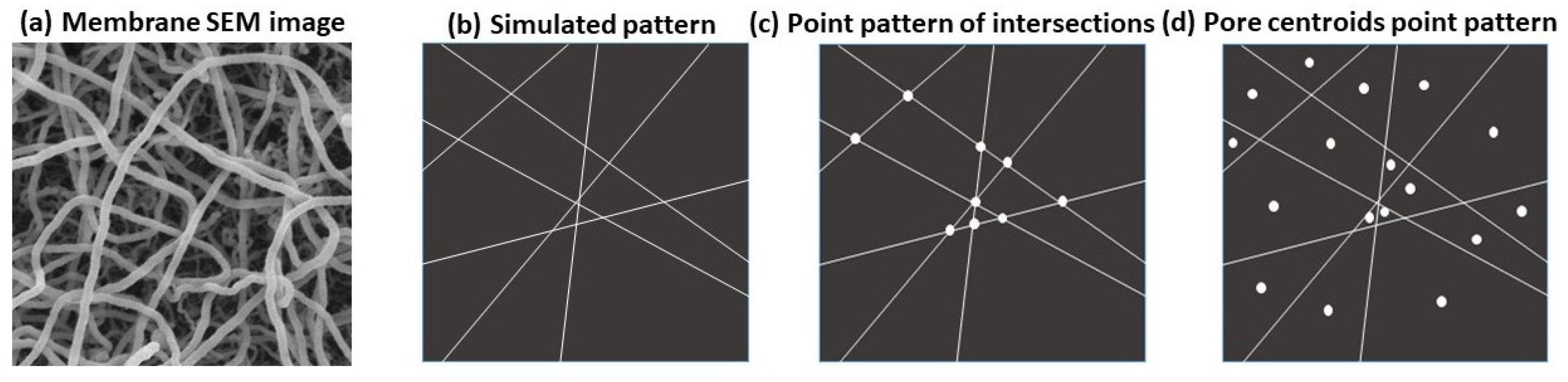
Analyzed SEM Images and Processing

The general computational flowchart for the processing of the SEM image dataset analyzed in this manuscript comprises the following steps. A median filter [40] is applied to the input grayscale image with a specified filter size. This operation serves to reduce salt and pepper noise while preserving edges and essential image features. Subsequent binarization of the image separates black pixels as pores and white as background. The thresholding parameter chosen for the binarization process is computed based on the grayscale image’s histogram morphology. For example, when the histogram is bimodal, the choice of the binarization threshold at the minimum between peaks is often successful.

To further refine the binary image, a morphological closing operation [41] is employed with a disk-shaped structuring element used for this purpose. This operation aids in the removal of small discontinuities and connects nearby structures. Small noise artifact holes within the binary image are then filled to ensure the continuity of segmented structures. As for the exterior boundaries of segmented pores, these are extracted using a built-in algorithm that employs 8-connectivity and omits holes in the boundary extraction process. To enhance pore identification, objects with an area below a specified threshold are classified as noise and removed from the segmented image, thereby updating the parameters of the segmented pores.

It should also be noted that SEM primarily analyzes surface pores by detecting secondary electrons. In our case, where the membrane is sufficiently thin, the surface pores observed can be indicative of the underlying 3D pore structure. This correlation is due to the lower tortuosity and higher effectiveness of thinner membranes in reflecting the true 3D architecture of the pores. Consequently, while SEM images provide valuable insights into the surface characteristics of fiber systems, the interpretation of these images must consider the limitations imposed by the projection of 3D structures onto a 2D plane in the cases where the membranes are not sufficiently thin [42].

3. Results

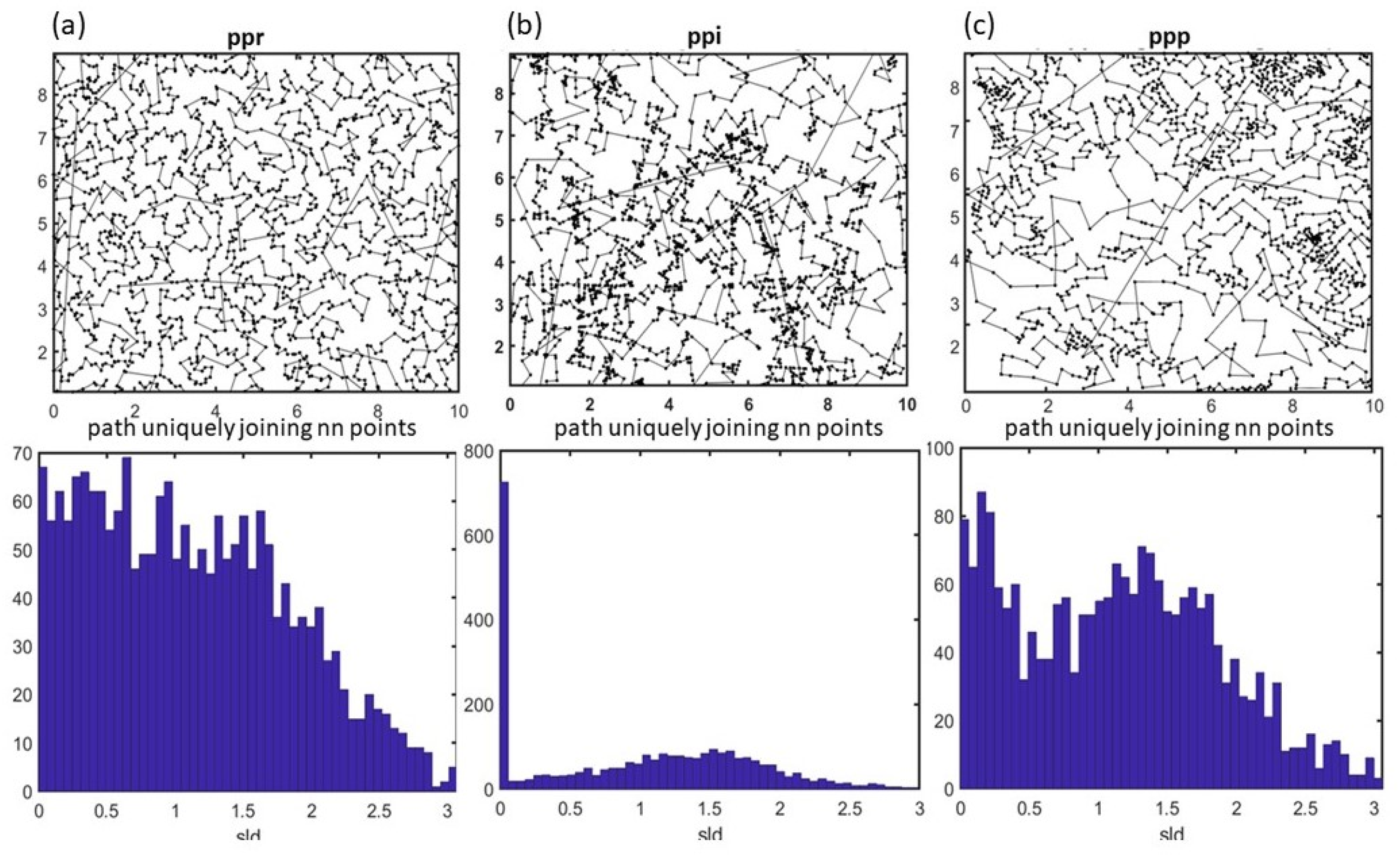
3.1. Characterizing Simulated Intersection and Pore Point Patterns

3.1.1. NNI

Figure 6 showcases the NNI for the ppi and ppp as a function of the number of randomly distributed straight lines. For the ppi, the values of NNI = 0.64–0.67 < 1 seem to indicate a strong clustering effect. Intuitively, this may be the result of the formation of intersection points created in close proximity with each other, as the creation of even one intersection indicates that at least two lines pass through that part of the inspection area, meaning that if even one more line passes close to the point of intersection, two more intersection points may be created. Figure 6a also shows that the NNI values remain in the short range of $0.64–0.67$, exhibiting small variability versus the number of lines and therefore the network density.

The results of the intersection point pattern NNI analysis align with the observations of Dodson [28] regarding the correlation between the lengths of adjacent sides of polygons arising from such Poisson line processes. This correlation, being independent of process intensity, which is proportional to number of lines, is related to how the spatial distribution of intersections influences the geometry of the polygons formed. For example, clustered intersection points are reflective of higher local line density, corresponding to shorter polygon sides. Thus, NNI offers another perspective of analytic approach for the estimation of local characteristics and inhomogeneities in line networks.

Figure 6b displays the relationship of NNI as a function of the number of lines for the ppp. In this case, we observe a different behaviour of the point pattern of the pores compared to the point pattern of the intersections, as the NNI index this time exceeds the barrier of 1 following an increasing trend, until it reaches a plateau at about 400 lines. This observation could be explained by the very nature of the pores. Simple calculation shows that n randomly placed lines intersect at ${\displaystyle \frac{n^2-n}{2}}$ different points and they form ${\displaystyle \frac{(n-1)(n-2)}{2}}$ pores. Therefore, in areas where more straight lines pass and intersect, more pores are created, which tend to have a smaller area. Consequently, small families of pores are created in these areas. However, because each pore is represented in the ppp as a point defined by the coordinates of its centroid, these pore centres are not clustered. This observation arises as a result of the fact that the pore centroids have at least a distance of each other analogous of their area, so they appear to repel each other, which translates to actually displaying order. Thus, this is a possible explanation for the higher than 1 NNI values found in ppp, and also for the increase of NNI with respect to the number of lines comprising the networks under study.

3.1.2. Nearest Neighbor Orientation Distribution

The rose plots of Figure 7 indicate the values of $\hat{\vartheta }\left(t\right)$ for the random point pattern ppr (a), ppi (b), and ppp (c) of pp created by 100 lines (analogous to 2000 points for the ppr). The values are distributed according to their numerical range, thus blue surfaces closer to the edge of the circle indicate that this direction is preferable, as it appears more frequently. In the rose plot for the ppr, the values are quite evenly distributed, as expected by the Poisson distribution of the points. A relatively uniform trend also appears in the case of the ppi. In contrast, the ppp exhibits more directionality, with the polar plot values leaning towards 330°. This preference, however, is ultimately virtual, as from the analysis of different ppps, there does not seem to exist a certain affinity to specific angles. Nevertheless, the results show that the distributions exhibit maxima, though the directions preferred in one iteration are not necessarily the same in another. This is an indication that directionality exists, though more work on its thorough analysis and interpretation is required.

As the number of lines increases, the number of intersections exhibits square growth, so the intersection points get closer and closer to each other; thus, it is more probable to find nearest neighbors in alignment with the typical point. In the case of the ppp, pores formed by lines that intersect with a slight inclination tend to have their center on the bisector of the angle formed by these two lines, thus showing alignment phenomena. This observation is visualized in Figure 8, where pore centroids (blue) seem to align with the bisector (yellow) of two lines crossed with a slight inclination.

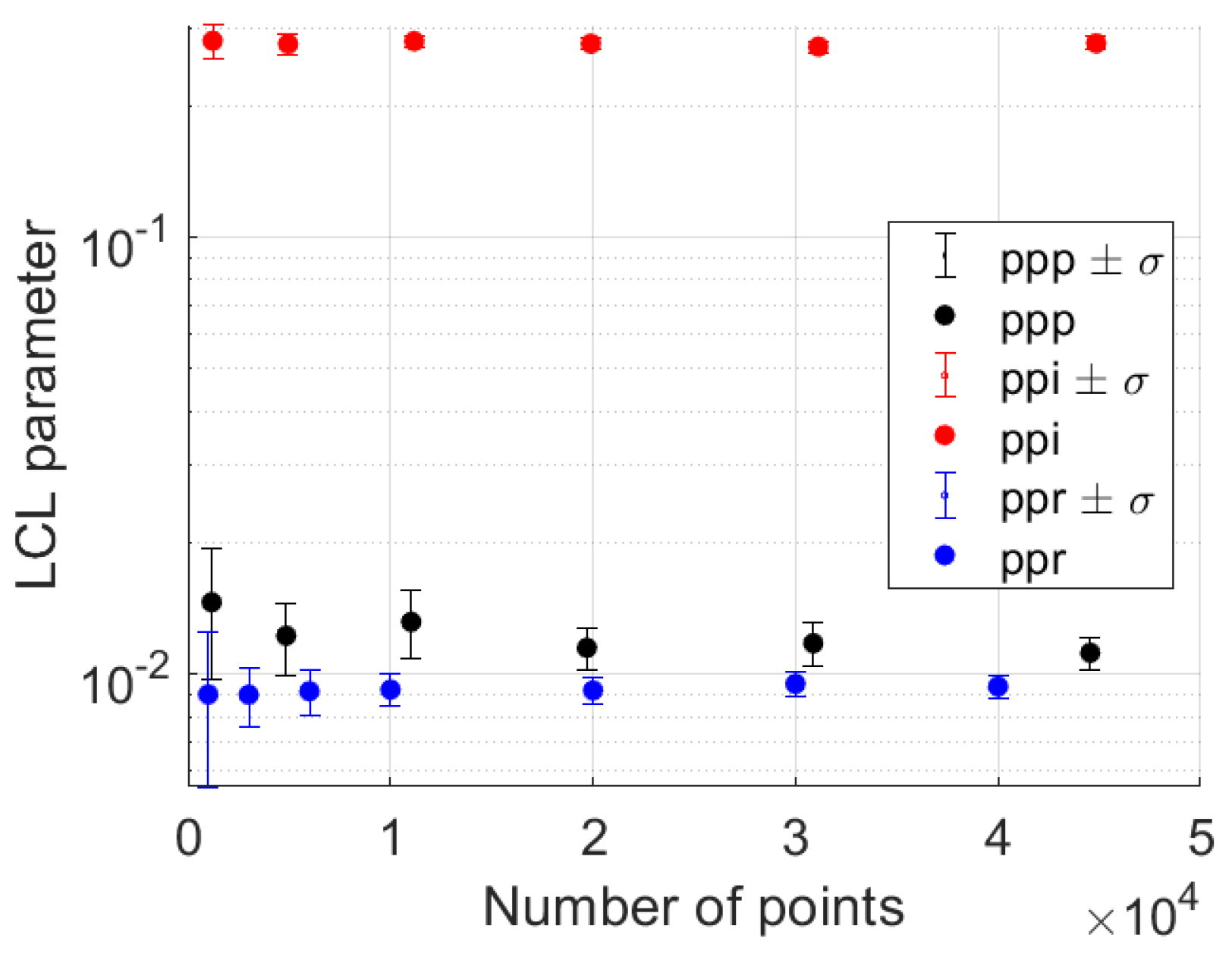
3.1.3. Local Collinearity

In Figure 9, three examples of ppr (a), ppi (b), and ppp (c), along with the paths uniquely joining nearest neighbor points of the patterns, are shown. In the second row of the figure, we plot the histograms of the slope differences values (sld) of consecutive line segments of the path (see Equation (5)). For the ppr, simple geometrical arguments can show that the histogram remains almost fixed till the value π/2 while for sld > π/2 falls sinusoidally following approximately the formula n_fixed − sin(sld − π/2), where n_fixed is the number of sld values at the fixed part of the histogram (sld < π/2). This analytical expression is the baseline of the sld histogram shape when complete spatial randomness is assumed.

Besides ppr, the spike of the histogram of ppi at zero indicates high collinearity, while the histogram of ppp is closer to ppr, both exhibiting more homogeneity in the sld values. Thus, these cases are to be further examined with the calculation of the LCL parameter (refer to Equation (6)) to find indications of collinearity phenomena in these patterns.

As for the influence of the starting point to the lcl path, multiple realizations of the path for different starting points on the same point pattern indicated a standard deviation of less than 10% for all cases of point patterns. Therefore, the choice of starting point can be random. To mitigate edge effects, the nearest neighbor edge correction method is applied to the point patterns in question by considering in the calculations all points with nearest neighbor distance lower than the smallest distance of the point from the borders of the observed area. Additively, in the case of the ppp, pores not fully contained within the observation area are excluded from the analysis.

Additionally, in Figure 9, while the peak at sld ≈ 0 is indicative of perfect collinearity, the distribution in the intermediate range of slope differences (approximately 0.75 to 2 radians) reveals a distinct behavior in both ppi and ppp patterns compared to the baseline ppr. This region represents configurations where three points are not exactly aligned but still demonstrate a constrained directional trend. In our main analysis, we focused primarily on the left side of the histogram (sld ≈ 0), as strict collinearity was the core requirement for defining the LCL parameter. As shown above, in the case of the random baseline pattern, up to 1.5 rad, a roughly flat distribution is observed and then a drop occurs. When the pattern has alignment effects (such as in the cases of ppi and ppp), sld increases close to 0. The more intense the presence of collinear points, the more distinct the peak in the 0.75–1.5 range.

In this work, our primary objective is to explore and validate the behavior of the LCL parameter in realistic stochastic systems, particularly those that mimic the randomness inherent in fibrous materials and nanowire networks. These systems are typically characterized by disordered or semi-random line arrangements, making random line processes an appropriate and representative model for establishing a metrological baseline.

That said, synthetic structured patterns—such as periodic grids or aligned (directional) lines—could serve as useful cases to showcase the sensitivity of the LCL index across the spectrum of spatial organization. Figure 10 presents an example pattern with lines exhibiting strong directionality (baseline line angle pi/4 with variance pi/15), along with the corresponding LCL paths for visualization purposes and the histograms of sld values for both the ppp and ppi patterns.

Figure 11 shows the results of the LCL method for the analysis of the ppr, ppi, and ppp, where each point is the average over the calculation of LCL parameter for 10 different initial patterns. The size of the LCL parameter for the random point pattern (ppr) appears to be fixed close to 0.01 regardless of the number of points. Moving on to the ppi, the LCL parameter also appears to be fixed regardless of the number of lines, and it is restricted between 0.26 and 0.285, exhibiting clear and strong collinearity. This is expected considering that the ppi is formed by intersections, thus sets of points common to a line are obviously expected to be collinear. Interesting results arise from the ppp (Figure 11), where the pores exhibit LCL parameter marginally above the random pp, though with certainty.

Nevertheless, a value of the LCL ratio below 0.01 suggests that the pp under study does not support collinear patterns resembling the ppr behavior.

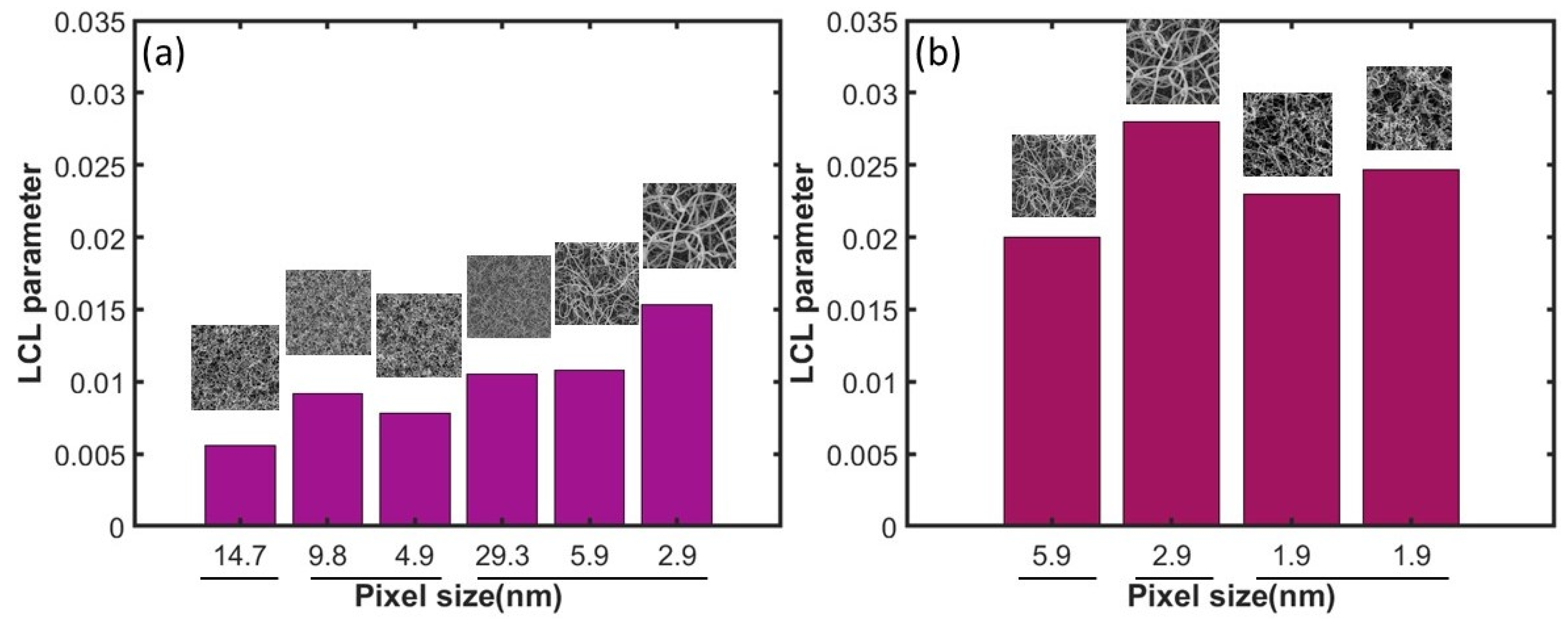
3.2. Characterizing Pore Point Patterns of Experimental Membrane Images

Analyzing the pore point pattern of a membrane offers a nuanced perspective that goes beyond conventional examinations of fiber arrangement effects. By focusing on the spatial distribution and arrangement of pores within the membrane, crucial insights into permeability, fluid dynamics, and filtration efficiency may be presented through the analysis of pore spatial arrangement through spatial statistics methods. Thus, in this case of the nanofilament coated PES membranes, materials of interest in filtration and water harvesting purposes, the application of the aforementioned methods is directly connected to the pore point pattern morphology, moving us towards a more comprehensive understanding of how fluids and particles traverse the membrane structure.

Figure 12a shows bar diagrams of the LCL parameter values obtained from the pore point patterns of the nanofilament coated PES membrane SEM images under study. SEM images of these membranes were taken at different magnifications, leading to the different pixel sizes (in nm). The lines underscoring and grouping the pixel size values indicate images taken at different magnification of the identical sample for clarity purposes. The LCL parameter values do not seem to be affected by magnification-number of fibers, as seen by the inconsistencies of the values in different pixel size images of the same sample. Apparently though, in agreement with the findings of the simulated cases in Figure 11, higher magnification images, thus an area of interest consisting of lower number of fibers/lines, exhibit bigger variability in LCL parameter values, as seen from the cases of 4.9, 5.9, and 2.9 nm pixel size images. This finding is consistent with the large standard deviation of LCL values from the simulated pattern results.

Our findings demonstrate that this slightly positive local collinearity (LCL) parameter indicates a tendency for pore alignment due to the intersection of fibers within the membrane. In water harvesting, optimized fluid dynamics can significantly improve the rate and volume of water harvested from sources such as fog, dew, or atmospheric moisture. Additionally, more uniform filtration is crucial for removing contaminants and ensuring the purity of the harvested water. Understanding these morphological characteristics is essential for designing and optimizing membranes specifically for water harvesting applications. By tailoring pore alignment to meet the unique demands of water harvesting, it is possible to develop membranes that maximize water collection efficiency while maintaining high standards of water quality.

In addition to the pore point patterns, we also performed an LCL analysis for the junction point patterns extracted from the same materials. These results are presented in Figure 12b. As expected, the LCL (ppi) values are higher than those of the LCL (ppp), reflecting the stronger tendency for collinear alignment among intersections formed along fiber trajectories. Interestingly, they are significantly lower than the simulated cases. This difference is attributed to intrinsic fiber geometry attributes, fiber curvature and tortuosity, and image thresholding bias during the image processing steps.

The joint analysis of LCL (ppp) and LCL (ppi) across multiple samples opens a promising avenue for characterizing the complexity of fibrous networks. A correlation between these parameters could indicate whether pore-level anisotropy stems directly from junction alignment, or whether additional structural factors such as local curvature and fiber tortuosity play a role. These insights can be pivotal for designing materials with tailored pore morphology or connectivity patterns.

4. Discussion

This study investigates the characteristics of point patterns in networks of randomly distributed lines, with a focus on two specific types: the intersections of lines and the centroids of pores. The aim is to provide valuable insights for the precise metrological characterization of fibrous networks and their structural properties, building a metrological framework for their quantification with stochastic geometry tools.

The results indicate that the intersection point patterns exhibit significant clustering, while the pore centroids are more uniformly distributed, showing a clear tendency toward periodicity. Intersection aggregation also relates to results regarding the correlation of lengths of polygons formed by the random line processes, as analyzed in Dodson [28]. Due to the line origins of the analyzed point patterns of intersections and pore centroids, special emphasis is given to their anisotropy and directionality characterization. To this end, we identify a gap in the characterization of collinearity phenomena and develop a novel methodology adapted to quantify the local collinearity of points in a point pattern. The resultant local collinearity parameter is obviously shown to obtain high values in the point patterns of intersections, indicating the strong presence of local collinear arrangements of intersection points. On the other side, pore centroids exhibit slighter local collinearity but clearly above the baseline of the local collinearity of random point patterns. Methodology application of collinearity investigation in experimental SEM images of membranes [32] offers insights into pore arrangement and highlights agreement with simulated cases.

Summing up the above findings, we can conclude that the point patterns of both intersections and pores of linear fiber networks show specific properties concerning their randomness and anisotropy/directionality, which should be considered in their modelling and experimental considerations. This avenue of investigation is poised to enhance our understanding of the intricate interplay between material structures and performance, ultimately fostering innovation and optimization in the design and utilization of fibrous materials for diverse applications.

This study examines an experimental case, where the point pattern of pores is of interest. Future work could focus on tailored solutions for other materials where, instead, the morphology of fiber intersections addresses the unique demands of specific materials, such as better conductivity or information dissemination.

Another approach could apply network analysis techniques, which can be used to study the properties of fiber networks, such as the number of nodes and edges, the degree of connectedness, and the presence of subnetworks or modules. This can provide information about the structure and function of the network and can be used to identify key nodes or pathways that may be important for network function.

References

1. Eichhorn, S.J.; Dufresne, A.; Aranguren, M.; Marcovich, N.E.; Capadona, J.R.; Rowan, S.J.; Weder, C.; Thielemans, W.; Roman, M.; Renneckar, S.; et al. Review: Current international research into cellulose nanofibres and nanocomposites. J. Mater. Sci. 2010, 45, 1–33. [Google Scholar] [CrossRef]
2. Paul, D.R.; Robeson, L.M. Polymer nanotechnology: Nanocomposites. Polymer 2008, 49, 3187–3204. [Google Scholar] [CrossRef]
3. Pham, Q.P.; Sharma, U.; Mikos, A.G. Electrospinning of polymeric nanofibers for tissue engineering applications: A review. Tissue Eng. 2006, 12, 11971211. [Google Scholar] [CrossRef]
4. Fu, W.; Liu, Z.; Feng, B.; Hu, R.; He, X.; Wang, H.; Yin, M.; Huang, H.; Zhang, H.; Wang, W. Electrospun gelatin/PCL and collagen/PLCL scaffolds for vascular tissue engineering. Int. J. Nanomed. 2014, 9, 2335–2344. [Google Scholar] [CrossRef] [PubMed]
5. Shen, H.; Zhou, Z.; Wang, H.; Zhang, M.; Han, M.; Durkin, D.P.; Shuai, D.; Shen, Y. Development of Electrospun Nanofibrous Filters for Controlling Coronavirus Aerosols. Environ. Sci. Technol. Lett. 2021, 8, 545–550. [Google Scholar] [CrossRef] [PubMed]
6. Alcoutlabi, M.; Lee, H.; Watson, J.V.; Zhang, X. Preparation and properties of nanofiber-coated composite membranes as battery separators via electrospinning. J. Mater. Sci. 2013, 48, 2690–2700. [Google Scholar] [CrossRef]
7. Cisneros, C.G.; Bloemen, V.; Mignon, A. Synthetic, Natural, and Semisynthetic Polymer Carriers for Controlled Nitric Oxide Release in Dermal Applications: A Review. Polymers 2021, 13, 760. [Google Scholar] [CrossRef]
8. Wang, S.; Liu, C.; Wang, F.; Yin, X.; Yu, J.; Zhang, S.; Ding, B. Recent Advances in Ultrafine Fibrous Materials for Effective Warmth Retention. Adv. Fiber Mater. 2022, 5, 847–867. [Google Scholar] [CrossRef]
9. Huang, X.L.; Dou, S.X.; Wang, Z.M. Fibrous cathode materials for advanced sodium-chalcogen batteries. Energy Storage Mater. 2022, 45, 265–280. [Google Scholar] [CrossRef]
10. Tadrist, L.; Miscevic, M.; Rahli, O.; Topin, F. About the use of fibrous materials in compact heat exchangers. Exp. Therm. Fluid Sci. 2004, 28, 193–199. [Google Scholar] [CrossRef]
11. Matsuo, T. Fibre materials for advanced technical textiles. Text. Prog. 2008, 40, 87–121. [Google Scholar] [CrossRef]
12. Sampson, W.W. Modelling Stochastic Fibrous Materials with Mathematica; Springer: London, UK, 2009. [Google Scholar]
13. Cho, Y.-S.; Roh, S.H. Sol–gel synthesis of porous titania fibers by electro-spinning for water purification. J. Dispers. Sci. Technol. 2018, 39, 33–44. [Google Scholar] [CrossRef]
14. Kulkarni, A.; Bambole, V.A.; Mahanwar, P.A. Electrospinning of Polymers, Their Modeling and Applications. Polym. Plast. Technol. Eng. 2015, 49, 427–441. [Google Scholar] [CrossRef]
15. Diaz-Alvarez, A.; Higuchi, R.; Sanz-Leon, P.; Marcus, I.; Shingaya, Y.; Stieg, A.Z.; Gimzewski, J.K.; Kuncic, Z.; Nakayama, T. Emergent dynamics of neuromorphic nanowire networks. Sci. Rep. 2019, 9, 14920. [Google Scholar] [CrossRef] [PubMed]
16. Hochstetter, J.; Zhu, R.; Loeffler, A.; Diaz-Alvarez, A.; Nakayama, T.; Kuncic, Z. Avalanches and edge-of-chaos learning in neuromorphic nanowire networks. Nat. Commun. 2021, 12, 4008. [Google Scholar] [CrossRef]
17. Jagota, M.; Tansu, N. Conductivity of Nanowire Arrays under Random and Ordered Orientation Configurations. Sci. Rep. 2015, 5, 10219. [Google Scholar] [CrossRef]
18. Kuncic, Z.; Nakayama, T. Neuromorphic nanowire networks: Principles, progress and future prospects for neuro-inspired information processing. Adv. Phys. X 2021, 6, 1894234. [Google Scholar] [CrossRef]
19. Lu, M.; Beguin, F.; Frackowiak, E. Supercapacitors: Materials. Systems and Applications; Wiley: Hoboken, NJ, USA, 2013. [Google Scholar]
20. Leong, K.F.; Chua, C.K.; Sudarmadji, N.; Yeong, W.Y. Engineering functionally graded tissue engineering scaffolds. J. Mech. Behav. Biomed. Mater. 2008, 1, 140–152. [Google Scholar] [CrossRef] [PubMed]
21. Dullien, F.A. Porous Media: Fluid Transport and Pore Structure; Academic Press: Cambridge, MA, USA, 2012. [Google Scholar]
22. Liu, Q.; Lu, Z.; Hu, Z.; Li, J. Finite element analysis on tensile behaviour of 3D random fibrous materials: Model description and meso-level approach. Mater. Sci. Eng. A 2013, 587, 36–45. [Google Scholar] [CrossRef]
23. Hull, R.; Keblinski, P.; Lewis, D.; Maniatty, A.; Meunier, V.; Oberai, A.A.; Picu, C.R.; Samuel, J.; Shephard, M.S.; Tomozawa, M.; et al. Stochasticity in materials structure, properties, and processing—A review. Appl. Phys. Rev. 2019, 5, 011302. [Google Scholar] [CrossRef]
24. Sampson, W.W. Spatial variability of void structure in thin stochastic fibrous materials. Model. Simul. Mater. Sci. Eng. 2011, 20, 015008. [Google Scholar] [CrossRef]
25. Eichhorn, S.J.; Sampson, W.W. Statistical geometry of pores and statistics of porous nanofibrous assemblies. J. R. Soc. Interface 2005, 2, 309–318. [Google Scholar] [CrossRef]
26. Miles, R.E. Random polygons determined by random lines in a plane, II. Proc. Nat. Acad. Sci. USA 1964, 52, 1157–1160. [Google Scholar] [CrossRef]
27. Abdel-Ghani, M.; Davies, G. Simulation of non-woven fibre mats and the application to coalescers. Chem. Eng. Sci. 1985, 40, 117–129. [Google Scholar] [CrossRef]
28. Dodson, C.T.J.; Sampson, W.W. Planar Line Processes for Void and Density Statistics in Thin Stochastic Fibre Networks. J. Stat. Phys. 2007, 129, 311–322. [Google Scholar] [CrossRef]
29. Chiu, S.N.; Stoyan, D.; Kendall, W.S.; Mecke, J. Stochastic Geometry and Its Applications; John Wiley & Sons: Hoboken, NJ, USA, 2013. [Google Scholar]
30. Barthélemy, M. Spatial networks. Phys. Rep. 2011, 499, 1–101. [Google Scholar] [CrossRef]
31. Illian, J.; Penttinen, A.; Stoyan, H.; Stoyan, D. Statistical Analysis and Modelling of Spatial Point Patterns; Wiley: Hoboken, NJ, USA, 2008. [Google Scholar]
32. Shah, P.; Hou, Y.; Butt, H.-J.; Kappl, M. Nanofilament-Coated Superhydrophobic Membranes Show Enhanced Flux and Fouling Resistance in Membrane Distillation. ACS Appl. Mater. Interfaces 2023, 15, 55119–55128. [Google Scholar] [CrossRef]
33. Dodson, C.T.J. Spatial variability and the theory of sampling in random fibrous networks. J. R. Stat. Soc. Ser. B 1971, 33, 88–94. [Google Scholar] [CrossRef]
34. Rajala, T.; Redenbach, C.; Särkkä, A.; Sormani, M. A review on anisotropy analysis of spatial point patterns. Spat. Stat. 2018, 28, 141–168. [Google Scholar] [CrossRef]
35. Pinder, D.A.; Witherick, M.E. The Principles, Practice and Pitfalls of Nearest-Neighbour Analysis. Geography 1972, 57, 277–288. [Google Scholar]
36. Philo, C.; Philo, P. 2.15 or Not 2.15? An Historical-Analytical Inquiry into the Nearest-Neighbor Statistic. Geogr. Anal. 2021, 54, 333–356. [Google Scholar] [CrossRef]
37. Mavrogonatos, A.; Papia, E.-M.; Constantoudis, V. Measuring the randomness of micro- and nanostructure spatial distributions: Effects of Scanning Electron Microscope image processing and analysis. J. Microsc. 2022, 289, 48–57. [Google Scholar] [CrossRef] [PubMed]
38. Myllymäki, M.; Mrkvička, T.; Grabarnik, P.; Seijo, H.; Hahn, U. Global Envelope Tests for Spatial Processes. J. R. Stat. Soc. Ser. B Stat. Methodol. 2017, 79, 381–404. [Google Scholar] [CrossRef]
39. Wiegand, T.; Grabarnik, P.; Stoyan, D. Envelope tests for spatial point patterns with and without simulation. Ecosphere 2016, 7, e01365. [Google Scholar] [CrossRef]
40. Brownrigg, D.R.K. The weighted median filter. Commun. ACM 1984, 27, 807–818. [Google Scholar] [CrossRef]
41. Ronse, C.; Heijmans, H.J.A.M. The algebraic basis of mathematical morphology: II. Openings and closings. CVGIP Image Underst. 1991, 54, 74–97. [Google Scholar] [CrossRef]
42. Papia, E.-M.; Constantoudis, V.; Ioannou, D.; Zeniou, A.; Hou, Y.; Shah, P.; Kappl, M.; Gogolides, E. Quantifying pore spatial uniformity: Application on membranes before and after plasma etching. Micro Nano Eng. 2024, 24, 100278. [Google Scholar] [CrossRef]
Figure 1. (a) Nanofilament coated PES SEM image [32]. (b) A simple line pattern simulating fiber structure. Examples of the two types of pp under study in this work: (c) the point pattern of the intersections of the fibers (ppi), and (d) the point pattern of the centroids of the pores (ppp).
Metrology 05 00026 g001
Figure 2. Example visualizations of point patterns exhibiting local anisotropy (a) and global anisotropy (b). The yellow circles highlight examples of triads of collinear points exhibiting local directionality and anisotropy though the whole point pattern is globally isotropic.
Metrology 05 00026 g002
Figure 3. (a) A line pattern consisting of 20 randomly placed straight line segments simulating fiber arrangement with indication of the pore centroids (red dots). (b) The LCL path formed by the ppp of the line pattern shown in (a). (c) The histogram of difference of slope values (10 bins), which distributes the slopes of all the point triads.
Metrology 05 00026 g003
Figure 4. Example visualization of three line segments connecting each point to its nearest neighbor. Each segment is named after its i-th point, and its consecutive segment as the (i + 1)-th point. The notations sl1 and sl2 indicate the slopes of line segments 1 and 2, respectively.
Metrology 05 00026 g004
Figure 5. Frequency counts vs. the number of collinear triplets for 1000 realizations of 1000-point random point patterns. The envelope is defined by the 2.5th and 97.5th percentiles marked with green dashed lines, while the observed/baseline count is defined by red solid line.
Metrology 05 00026 g005
Figure 6. NNI as a function of the number of lines for the ppi (a) and ppp (b). One can notice the independence of NNI of ppi from number of lines at values smaller than 1 revealing strong clustering effects in ppi and the increasing trend of NNI of ppp towards a saturation value higher than 1 indicating the trend towards periodicity in ppp.
Metrology 05 00026 g006
Figure 7. Rose plots that indicate the values of the nearest neighbor orientation distribution function ϑ ˆ ( t ) for the ppr (a), ppi (b), and ppp (c) of a pp created by 100 lines (analogous to 3000 points for the ppr).
Metrology 05 00026 g007
Figure 8. Visualization of a line pattern, where pore centroids (blue star shapes) seem to align with the bisector (yellow) of two lines crossed with a slight inclination.
Metrology 05 00026 g008
Figure 9. Three examples of point patterns, (a) ppr (2000 points), (b) ppi (100 lines), and (c) ppp (100 lines), with their paths uniquely joining their nearest neighbor points (top row) and the histograms (50 bins) of the sld values of the paths (bottom row).
Metrology 05 00026 g009
Figure 10. (a) Example pattern with lines exhibiting strong directionality (baseline line angle pi/4 with variance pi/15), along with the corresponding LCL path (b) for the ppp and (c) ppi for visualization purposes and the histograms of sld values for both the (d) ppp and (e) ppi patterns.
Metrology 05 00026 g010
Figure 11. Results of the LCL method showing LCL parameters from the analysis of the ppp (black), ppi (red), and ppr (blue), where each point is the average over the calculation for 10 different initial patterns.
Metrology 05 00026 g011
Figure 12. Bar diagrams per pixel size (in nm) in nanofilament coated PES membrane SEM images for the LCL parameter values obtained from the pore point patterns (a) and intersection point patterns (b) of each image. The lines underscoring and grouping the pixel size values indicate images of the same material sample.
Metrology 05 00026 g012