Using a Multivariate Virtual Experiment for Uncertainty Evaluation with Unknown Variance

Abstract

Virtual experiments are a digital representation of a real measurement and play a crucial role in modern measurement sciences and metrology. Beyond their common usage as a modeling and validation tool, a virtual experiment may also be employed to perform a parameter sensitivity analysis or to carry out a measurement uncertainty evaluation. For the latter to be compliant with statistical principles and metrological guidelines, the procedure to obtain an estimate and a corresponding measurement uncertainty requires careful consideration. We employ a Monte Carlo sampling procedure using a virtual experiment that allows one to perform a measurement uncertainty evaluation according to the Monte Carlo approach of JCGM-101 and JCGM-102, two widely applied guidelines for uncertainty evaluation in metrology. We extend and formalize a previously published approach for simple additive models to account for a large class of non-linear virtual experiments and measurement models for multidimensionality of the data and output quantities, and for the case of unknown variance of repeated measurements. With the algorithm developed here, a simple procedure for the evaluation of measurement uncertainty is provided that may be applied in various applications that admit a certain structure for their virtual experiment. Moreover, the measurement model commonly employed for uncertainty evaluation according to JCGM-101 and JCGM-102 is not required for this algorithm, and only evaluations of the virtual experiment are performed to obtain an estimate and an associated uncertainty of the measurand. We demonstrate the efficacy of the developed approach and the effect of the underlying assumptions for a generic polynomial regression example and an example of a simplified coordinate measuring machine and its virtual representation. The results of this work highlight that considerable effort, diligence, and statistical considerations need to be invested to make use of a virtual experiment for uncertainty evaluation in a way that ensures equivalence with the accepted guidelines.

1. Uncertainty Evaluation Using a Virtual Experiment

Virtual experiments are mathematical and numerical models representing a physical measurement process in a virtual environment. In an ideal scenario, a virtual experiment is able to generate virtual observations with the same statistical properties as the observations of the corresponding real experiment [1]. Similar to digital twins [2,3], virtual experiments have gained significant popularity in industry [4,5,6,7,8] and wider measurement science [9] with a variety of use-cases. In contrast to a digital twin, a virtual experiment lacks the ‘twinning’ with the real experiment that would allow it to continuously update the virtual representation based on feedback from the real counterpart and vice versa. However, a virtual experiment is an essential, but static, element of a digital twin with several applications of its own. While virtual experiments can be used to improve the measurement processes itself and explore significant error sources using a sensitivity analysis [10], one of the key applications is the evaluation of measurement uncertainty [11,12,13], which we will focus on in this work.

Here, we consider virtual experiments of a specific (semi-) non-linear structure with an additive Gaussian noise error term

$$X^{\mathrm{ve}}=\mathrm{VE}(Y,Z;\Sigma )=g(Y,Z)+ϵ=A\left(Z\right)Y+B\left(Z\right)+ϵ,ϵ\sim N(0,\Sigma ),\Sigma =\mathrm{diag}({\sigma }_1^2,\dots ,{\sigma }_n^2).$$

(1)

A general introduction to virtual experiments and a similar class of models is considered in [14] for the univariate case, and in [11], additive virtual experiments have been analyzed.

Table 1. Overview of symbols, quantities, and parameters used in this work.

Symbol	Description	Comment
$Y=(Y_1,\dots ,Y_p)$	Quantity for the measurand having $p\ge 1$ elements.	Quantity of interest for which an estimate and associated uncertainty is to be derived.
Z	Parameter for which Type-B information is available in terms of a state-of-knowledge PDF $\pi \left(z\right)$.	Possibly multivariate and its value is considered to be unknown but fixed in the real experiment.
$\mathbf{x}=({\mathbf{x}}_1,\dots ,{\mathbf{x}}_m)$, ${\mathbf{x}}_i=(x_i^1,\dots ,x_i^n)$	Observations in the real experiment. We assume $m\ge 1$ independent observations, each of dimension $n\ge 1$.	To circumvent ill-posedness, we assume $m>p$ and to ensure the existence of the JCGM-102 input PDF, also $m>n$.
$ϵ=({ϵ}_1,\dots ,{ϵ}_n)$	Statistical error term. Here, we consider only the additive case.	Realizations of a normal distribution $N(0,\Sigma )$ might not be known to the user of the virtual experiment.
$\Sigma =\left[\begin{array}{ccc}{\sigma }_1^2& & \\ & \ddots & \\ & & {\sigma }_n^2\end{array}\right]$	Covariance used in virtual experiment to model statistical variability in repeated measurements.	Variances ${\sigma }_1^2,\dots ,{\sigma }_n^2$ are known to the user of the virtual experiment.

presents an overview of the quantities required in this work. In (1), Y denotes the measurand, which is the $p\ge 1$ dimensional quantity of interest in the measurement and also the quantity for which an estimate and corresponding uncertainty has to be obtained. In the examples considered in Section 4, Y corresponds to either a set of polynomial coefficients, cf. Section 4.1, or the radius and position of a circle estimated from coordinate measurements, cf. Section 4.2. By Z, we denote the set of fixed parameters that are identified to affect the measurement and hence the virtual experiment, e.g., instrument setup parameter, temperature effects, reference quantities, and additional error terms, and about which non-statistical information is available. These quantities are unknown in a real experiment. Having values for these two quantities Y and Z, realizations of the $n\ge 1$ dimensional virtually measured quantity $X^{\mathrm{ve}}$ can be obtained by evaluation of the virtual experiment (1). The uncertainty due to repetition of the experiment is reflected by $ϵ$, which we model here as an additive Gaussian noise with diagonal covariance matrix $\Sigma \in {\mathbb{R}}^{n,n}$. This additive error model is a common modeling choice in measurement science [15,16], statistics [17], and uncertainty quantification [18,19] that obviously is a simplification for real and complex measurement procedures. While the values of the variances ${\sigma }_1^2,\dots ,{\sigma }_n^2$ of repetitions in the virtual experiment need to be specified and provided by the user, we assume here that the actual realization of $ϵ$ might not be accessible for the user when evaluating the virtual experiment. This might be the case when the virtual experiment is a black-box software tool that internally generates noisy observations of some quantity. However, the values for the measurand Y, the parameter Z, and the assumed covariance $\Sigma$ are provided. The forward model g is usually a complex function that mimics the measurement process, e.g., by simulating physical phenomena by the solution of differential equations or the operating mode of sensors. In this work, we additionally assume that the forward model g can be written as a function $A\left(Z\right)Y+B\left(Z\right)$, which is linear in the measurand quantity Y and non-linear in the parameter vector Z. The functions A and B depend on the applications involved and map (elements of) the parameter vector Z to ${\mathbb{R}}^{n,p}$ and ${\mathbb{R}}^n$, respectively. This class of models could also include additive terms accounting for model inadequacy as suggested in [20] based on a model calibration. The class of virtual experiments considered here is multivariate, in contrast to the previous literature [14], and allows more realistic and involved modeling. Virtual experiments of the form (1) can, for instance, be found in dimensional metrology when considering coordinate measuring machines [7,12] or when simulating the pressure of a flow in a porous media [21]. Also, many surrogate models, such as proper orthogonal decompositions [22], Karhunen–Loeve expansions [23], and multilinear tensor formats [24] fall within this category.

To use a virtual experiment for uncertainty evaluation in conjunction with a set of real observations, a Monte Carlo procedure can be employed [25] that repeatedly applies the virtual experiment (1) for different realizations of the virtual system, i.e., the parameter vector Z. Then, the resulting spread of the virtual observations can be analyzed. However, in a real experiment, it is usually assumed that repeated measurements are taken from a specific instrument with a fixed value for the Z parameters and the part of the uncertainty due to repeatability is reflected by random influences that cannot be controlled in the measurement, i.e., the random vector $ϵ$. This conceptual difference between a real and virtual experiment has been pointed out before [11], and an alternative application of the virtual experiment for the purpose of uncertainty evaluation has been analyzed [13].

The goal of this work is to derive a simple Monte Carlo sampling procedure that solely requires application of the virtual experiment (1) to perform uncertainty evaluation for the measurand, following the two guidelines JCGM-101 [26] and JCM-102 [27] for uncertainty evaluation in metrology, without explicitly requiring a measurement model. However, the approach should produce an estimate and associated uncertainty of the measurand Y that is equivalent to the results produced by applying JCGM-101 or JCGM-102. The procedure in this work is particularly interesting and applicable when the virtual experiment is a black-box and might involve complex mathematical and numerical computations since the derived algorithm does not require explicit knowledge about the elements of the virtual experiment (1), i.e., $A\left(Z\right),B\left(Z\right),$ and $ϵ$, which would be required to build a corresponding measurement model for uncertainty evaluation according to the GUM.

This manuscript is organized as follows: we recall the JCGM-102 Monte Carlo procedure in Section 2, and in Section 3, we derive an equivalent Monte Carlo sampling procedure using only the virtual experiment. Numerical examples in Section 4 show the validity of the proposed approach.

2. The Reference Monte Carlo Procedure According to the JCGM-102

In the JCGM-102 and related GUM documents, a set of independent, real observations and a measurement model are required to perform an uncertainty evaluation. The $m\ge 1$ repeated observations ${\mathbf{x}}_1,\dots ,{\mathbf{x}}_m$ are taken for the $n\ge 1$ observed quantities, i.e., every observation ${\mathbf{x}}_i=(x_i^1,\dots ,x_i^n)$ is a vector that may represent different measurement locations, wavelengths, or parameter settings, depending on the application considered. The corresponding quantity for which the observations are assumed to be realizations of is denoted by X, and it is required to have more observations than dimensions $m>n$. The measurement model, which relates the input quantities X and additional parameters Z to the measurand Y, is denoted by f. A possible choice for the measurement model based on the form of the virtual experiment (1) can be formulated assuming that the function A in (1) has a pseudo-inverse for reasonable values of Z by

$$Y=f(X,Z)=A{\left(Z\right)}^{-1}(X-B\left(Z\right)).$$

(2)

However, especially in higher dimensions, the choice of the measurement model can be challenging, and even though the measurement model (2) is taken as the partial inverse of the virtual experiment (1), this is by no means the only option and ambiguous. In fact, the measurement model can deviate from the choice in (2) and we will analyze this in the example of a coordinate measuring machine in Section 4.2. Furthermore, the measurement model f is conceptually different from the virtual experiment (1) and the involved forward model g [11]. In the former, the quantity corresponding to the measurement data is entered as an input, while the latter produces virtual data assuming a value for the measurand Y and the Z parameters.

For the JCGM-102 Monte Carlo approach, we assume there is some measurement model (2) given and a probability density function (PDF) $\pi \left(z\right)$ for the quantity Z, which may be the result of expert elicitation or the explicit guidance in JCGM-101 [26]. For the measured quantity X, JCGM-102 assigns in clause 5.3.2 a multivariate scaled and shifted t-distribution with $\nu =m-n$ degrees of freedom. The shift by the experimental mean vector and the scaling through the scaled experimental covariance are based on the observations ${\mathbf{x}}_1,\dots ,{\mathbf{x}}_m$. In particular, one assigns

$$\pi \left(x\right)=t_{\nu }(\overline{x}=({\overline{x}}^1,\dots ,{\overline{x}}^n),S/m),{\overline{x}}^j={\displaystyle \frac{1}{m}}\sum _{i=1}^m{x}_i^j,S={\displaystyle \frac{1}{\nu }}\sum _{i=1}^m({\mathbf{x}}_i-\overline{x}){({\mathbf{x}}_i-\overline{x})}^T,$$

(3)

where $t_{\nu }$ denotes the PDF of the corresponding multivariate t distribution. Sampling from the multivariate scaled and shifted t-distribution can be accomplished by sampling from a multivariate standard normal distribution and scaling and shifting the samples accordingly. In particular, for a random vector $\theta$ following a multivariate normal distribution with mean $\mu$, covariance ${\Sigma }_N$, and $\eta$ following a multivariate scaled and shifted t-distribution as in (3), the following equality (this equality holds in distribution, which means, the random vector on the left-hand side and the random vector on the right-hand side of the equality symbol follow the same distribution) holds:

$$\eta =S^{1/2}{\displaystyle \frac{{\Sigma }_N^{-1/2}(\theta -\mu )}{\sqrt{\phi }}}{\displaystyle \frac{\sqrt{\nu }}{\sqrt{m}}}+\overline{x},\eta \sim t_{\nu }(\overline{x},S/m),\theta \sim N(\mu ,\Sigma ),\phi \sim {\chi }^2\left(\nu \right).$$

(4)

Here, $\phi$ is a random variable that follows a ${\chi }^2$-distribution with $\nu$ degrees of freedom. The matrix square roots of the symmetric positive definite covariance matrices S and ${\Sigma }_N$ can be obtained, for example, by the Cholesky decomposition. This means that drawing samples from a t-distribution can be realized by combining samples from a normal distribution with samples from a ${\chi }^2$-distribution. For more details, cf. [27] (clause 5.3.2.4) and [28].

At this point it is to note that the requirement $m>n$, i.e., assuming more observations than dimensions in the observed quantity, can be omitted when assuming a known covariance of the observations. In this case, a multivariate normal distribution with estimate $\overline{x}$ can be assigned instead of a multivariate t-distribution [26] (clause 6.4.8). This includes the case of $m=1$, which is commonly considered for the coordinate measuring machine. However, in this work, we focus on the case of an unknown covariance in the observations.

Based on this PDF assignment for the quantity X and the availability of a PDF for the quantity Z, the following Monte Carlo sampling Algorithm 1 may be applied to approximate the state-of-knowledge distribution for the measurand.

Algorithm 1 JCGM-102 Monte Carlo algorithm

Input:  Measurement model $f(X,Z)$, real observations ${\mathbf{x}}_1,\dots ,{\mathbf{x}}_m$, state-of-knowledge PDF $\pi \left(z\right)$, number of samples N. Output:  Samples from state-of-knowledge PDF of measurand $\pi \left(Y\right)$  1: Compute state-of-knowledge PDF $\pi \left(x\right)$ for the quantity X as in (3)  2: for  $i=1,\dots ,N$  do  3:     $z_i^{\prime }\leftarrow$ Draw sample from PDF $\pi \left(z\right)$  4:     $x_i^{\prime }\leftarrow$ Draw sample from PDF $\pi \left(x\right)$  5:     $y_i^{\prime }\leftarrow$ Evaluate measurement model $f(x_i^{\prime },z_i^{\prime })$  6: end for  7: Summarize samples $y_1^{\prime },\dots ,y_N^{\prime }$ to obtain estimate and corresponding uncertainty in terms of the mean vector and the covariance matrix $$\widehat{y}={\displaystyle \frac{1}{N}}\sum _{i=1}^N{y}_i^{\prime },U_Y={\displaystyle \frac{1}{N-1}}\sum _{i=1}^N(y_i^{\prime }-\widehat{y}){(y_i^{\prime }-\widehat{y})}^T.$$ (5)  8: The standard uncertainty of every element of Y is given by the square root of the diagonal elements of $U_Y$.

In the following section, we derive a similar Monte Carlo sampling algorithm that, under the assumed structure of the virtual experiment (1) and measurement model (2), yields the same state-of-knowledge PDF as JCGM-102 in Algorithm 1. However, we only require the application of the virtual experiment (1) and a suitable transformation of its output.

3. A Monte Carlo Sampling Procedure Using the Virtual Experiment

There are two main issues when using a virtual experiment, as in (1), for uncertainty evaluation for the measurand. Firstly, every evaluation of the virtual experiment requires a value for the measurand as input. Since the true value for the measurand is generally unknown, virtual observations generated by the virtual experiment will most likely differ from real observations. For the algorithm developed later in this section, we will show that any simulated value $y_0$ for the measurand can be taken, without affecting the resulting estimate and its associated uncertainty. Secondly, repeated realizations from the virtual experiment are drawn from a multivariate normal distribution with assumed known covariance matrix $\Sigma$ and uncorrelated elements. On the other hand, the JCGM-102 approach considers a multivariate t-distribution and considers correlations, which are informed by real observations with unknown variances. Assuming the virtual experiment is a black-box and the distribution of the random deviations, represented by $ϵ$ in (1), cannot be altered, the random variable $X^{\mathrm{ve}}$ in (1) needs to be corrected to comply with the JCGM-102 Monte Carlo sampling approach. For this, the mean of the virtual experiment is required, i.e, for some value of the measurand y and some value of the parameter vector z, one either has direct access to the forward model $\mu :=g(y,z)$ or alternatively, one may estimate the mean from additional evaluations of the virtual experiment and a Monte Carlo estimate using many samples, here denoted by $N_{\mathrm{ve}}$

$$\mu =g(y,z)=\mathbb{E}\left[\mathrm{VE}(y,z;\Sigma )\right]\approx {\displaystyle \frac{1}{N_{\mathrm{ve}}}}\sum _{j=1}^{N_{\mathrm{ve}}}\left(g(y,z)+{ϵ}_j\right)$$

(6)

Additionally, for the following Monte Carlo Algorithm 2 to generate the same PDF as JCGM-102 and Algorithm 1, we require knowledge of $A\left(Z\right)$ from the virtual experiment to transform between the observations and the measurand. Since $A\left(Z\right)$ might be inaccessible in a black-box virtual experiment, it may be obtained by assuming that the virtual experiment also outputs a partial derivative. This derivative may be the derivative of the forward model g with respect to the measurand $J^{\mathrm{ve}}(y_0,z):={\displaystyle \frac{\partial g}{\partial y}}(y,z){|}_{y=y_0}$ evaluated at some value for the measurand $y_0$ and any z. Alternatively, the virtual experiment returns for every evaluation of (1) a realization and the corresponding disturbed partial derivative such that one may estimate for some $N_{\mathrm{ve}}$ that is large enough using

$$J^{\mathrm{ve}}(y_0,z)=A\left(z\right)={\displaystyle \frac{\partial }{\partial y}}g(y,z){|}_{y=y_0}=\mathbb{E}\left[{\displaystyle \frac{\partial \mathrm{VE}}{\partial y}}{(y,z;\Sigma )|}_{y=y_0}\right]\approx {\displaystyle \frac{1}{N_{\mathrm{ve}}}}\sum _{j=1}^{N_{\mathrm{ve}}}\left({\displaystyle \frac{\partial }{\partial y}}{g}_{{ϵ}_j}{(y,z)|}_{y=y_0}\right),$$

(7)

where $g_{{ϵ}_j}(y,z)$ denotes the disturbed output of the virtual experiment using some ${ϵ}_j\sim N(0,\Sigma )$, from which the gradient has to be obtained. Both cases are realistic in the sense that a black-box virtual experiment might directly return the gradient of the forward model since it may have been an essential part of the computations required, e.g., when g involves some optimization functional. Also, samples of a disturbed gradient might be present when an automatic differentiation tool is used after evaluation of the virtual experiment or when a gradient approximation is performed using finite difference methods.

Algorithm 2 Virtual experiment Monte Carlo algorithm.

Input:  Virtual experiment as in (1), real observations ${\mathbf{x}}_1,\dots ,{\mathbf{x}}_m$, state-of-knowledge PDF $\pi \left(z\right)$, number of samples of measurand N, simulated value of measurand $y_0$, covariance used in virtual experiment $\Sigma =\mathrm{diag}({\sigma }_1^2,\dots ,{\sigma }_n^2)$. Output:  Samples from state-of-knowledge PDF of measurand $\pi \left(y\right)$ with the same mean and covariance estimate as in Algorithm 1.  1: Estimate experimental mean vector $\overline{x}$ and scaled experimental covariance S as given in (3)  2: $L{L}^T=S/m\leftarrow$ compute Cholesky decomposition of $S/m$  3: for  $i=1,\dots ,N$  do  4:     $z_i^{\prime }\leftarrow$ Draw sample from PDF $\pi \left(z\right)$  5:     ${\overline{x}}_i^{\mathrm{ve}}\leftarrow$ experimental mean of m virtual experiment realizations $${\overline{x}}_i^{\mathrm{ve}}={\displaystyle \frac{1}{m}}\sum _{j=1}^m\mathrm{VE}(y_0,z_i^{\prime };\Sigma )={\displaystyle \frac{1}{m}}\sum _{j=1}^m\left(g(y_0,z_i^{\prime })+{ϵ}_j\right)$$ (8)  6:     ${\mu }_i\leftarrow$ get mean estimate from virtual experiment according to (6)  7:     $J_i\leftarrow$ get gradient estimate from virtual experiment according to (7)  8:     $c_i\leftarrow$ sample a single realization from a ${\chi }^2$ distribution with $\nu =m-n$ degrees of freedom  9:     $T_i\leftarrow$ create transformation matrix to correct for unknown variances according to (4) $$T_i=L\mathrm{diag}\left({\displaystyle \frac{\sqrt{\nu m}}{{\sigma }_1\sqrt{c_i}}},\dots ,{\displaystyle \frac{\sqrt{\nu m}}{{\sigma }_n\sqrt{c_i}}}\right)$$ (9) 10:     $y_i^{\prime }\leftarrow$ obtain corrected sample from desired PDF by $$y_i^{\prime }=J_i^{-1}\left(T_i({\mu }_i-{\overline{x}}_i^{\mathrm{ve}})+(\overline{x}-{\mu }_i)\right)+y_0,$$ (10) where $J_i^{-1}$ denotes the left (pseudo) inverse of $J_i$. 11: end for 12: Summarize samples $y_1^{\prime },\dots ,y_N^{\prime }$ to obtain estimate and uncertainty in terms of mean and covariance matrix $$\widehat{y}={\displaystyle \frac{1}{N}}\sum _{i=1}^N{y}_i^{\prime },U_Y={\displaystyle \frac{1}{N-1}}\sum _{i=1}^N(y_i^{\prime }-\widehat{y}){(y_i^{\prime }-\widehat{y})}^T.$$ (11) 13: The standard uncertainty of every element of Y is given by the square-root of the diagonal elements of $U_Y$.

With these ingredients, we present the following Monte Carlo sampling Algorithm 2, based only on the evaluation of a virtual experiment, that yields the same state-of-knowledge PDF for the measurand as the JCGM-102 Monte Carlo sampling approach.

Algorithm 2 effectively produces samples from the same distribution as the Monte Carlo sampling approach of JCGM-102 in Algorithm 1 using the measurement model (2). This is because Equation (10) corrects the assumed variances ${\sigma }_1^2,\dots ,{\sigma }_n^2$ to the t-distribution that accounts for the assumption of an a priori unknown variance of the data distribution, and also implicitly applies the measurement model (2). This means that Algorithm 2 prescribes the employed measurement model. However, for Algorithm 2, we only require evaluations of the virtual experiment and its gradient. In particular, no explicit knowledge about the possible highly non-linear additive term $B\left(Z\right)$ is required, and realizations of the virtual experiment might be noisy. In case the mean of the virtual experiment (6) and the gradient (7) need to be estimated from samples, the complexity of the Monte Carlo sampling in Algorithm 2 is $\mathcal{O}\left(N{N}_{\mathrm{ve}}\right)$ and the inversion of $J_i$, e.g., using least-squares estimation, can be performed in $\mathcal{O}\left(p^{2}n\right)$. Since N is usually much larger than the dimension of the measurand p and the dimension of the data vector n, the Algorithm 2 has asymptotically the computational complexity $\mathcal{O}\left(N{N}_{\mathrm{ve}}\right)$. If the variability of the observations and the measurand are of similar magnitude, one can safely consider $N=N_{\mathrm{ve}}$ since the convergence of a Monte Carlo estimate depends on the variance of the underlying random variables [29].

A note on generalization beyond the classes of measurement models considered here: the Algorithm 2 developed in Section 3 yields samples of the same PDF as JCGM-102 and Algorithm 1 under the assumption that the virtual experiment and the measurement model follow the structure of (1) and (2), respectively. For more general classes of virtual experiments and measurement models, the approach presented can be seen as a linearization procedure that considers, for every realization of the quantity Z, a local linearization in the measurand Y. The effect of taking a non-linear measurement model and a linearized virtual experiment is analyzed for the coordinate measuring machine in Section 4.2. A suitable alternative approach that may account for these kinds of models is a Bayesian approach, employing a statistical model based on the virtual experiment (1). This, however, is beyond the scope of this work.

4. Examples

In this section, we apply the developed uncertainty evaluation approach based on a virtual experiment (the implementations can be found here: https://gitlab1.ptb.de/marsch02/multivariate-ve (accessed on 17 September 2024)).

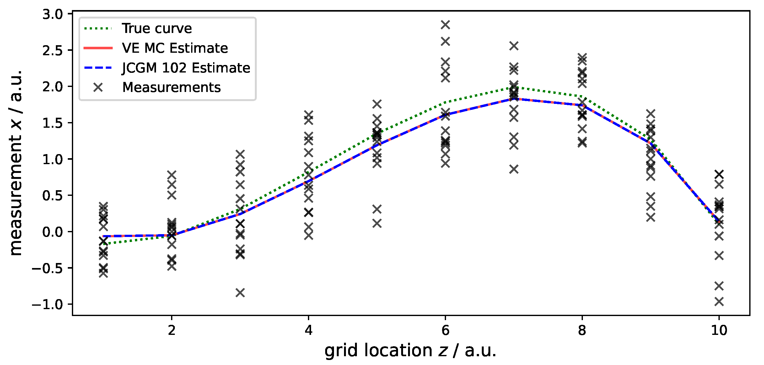
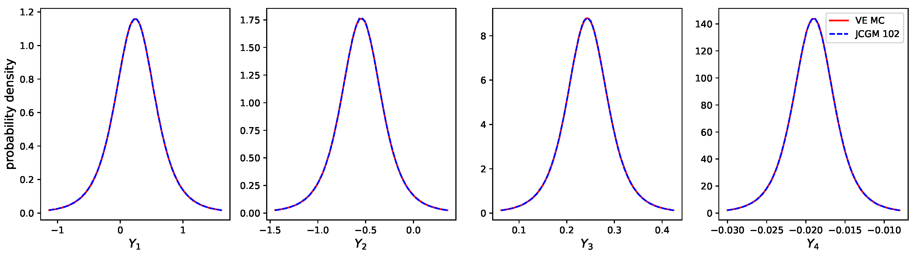
4.1. Generic Example Using Polynomial Regression

We first consider a generic example that reflects multivariate observations of a cubic polynomial at n unknown measurement locations. In particular, a virtual experiment is assumed that models these observations as realizations of the following form:

$$x^{\mathrm{ve}}=\left[\begin{array}{c}{x}_1^{\mathrm{ve}}\\ ⋮\\ x_n^{\mathrm{ve}}\end{array}\right]=\left[\begin{array}{cccc}1& z_1& z_1^2& z_1^3\\ & ⋮& & \\ 1& z_n& z_n^2& z_n^3\end{array}\right]\left[\begin{array}{c}{y}_1\\ y_2\\ y_3\\ y_4\end{array}\right]+\left[\begin{array}{c}{ϵ}_1\\ ⋮\\ {ϵ}_n\end{array}\right]{ϵ}_1,\dots ,{ϵ}_n\stackrel{\mathrm{iid}}{\sim }N(0,{\sigma }^2)$$

(12)

with ${ϵ}_1,\dots ,{ϵ}_n$ being independently and identically normally distributed with standard deviation $\sigma >0$ for the repeated realizations. The quantities, $Z_1,\dots ,Z_n$, corresponding to the values $z_1,\dots ,z_n$, represent measurement locations that are measured with an uncertainty. For the purpose of illustration, we assume $n=10$, and for each $Z_i$, a rectangular distribution centered at the measurement location i and a half-width of $0.1$ in arbitrary units is assigned for $i=1,\dots ,n$. This interprets every quantity corresponding to a measurement location as a quantity with Type-B information. This is related to the classical formulation of errors-in-variables problems for regression with uncertainty in both variables [30]. However, we assume that the uncertainty of the $Z_i$ does not contribute to the variability of repeated measurements and consider that the actual measurement locations are fixed for repeated measurements. For an in-depth analysis of errors-in-variables problems in metrology, cf. e.g., [31].The measurand, denoted by the quantity $Y=(Y_1,\dots ,Y_4)$ and values $y=(y_1,\dots ,y_4)$, are the polynomial coefficients and are to be determined in the following.

For the available observations of the real experiment ${\mathbf{x}}_1,\dots ,{\mathbf{x}}_m$, we assume that the data in Figure 1 has been observed with $m=12$ repetitions for each measurement location independently. The true but unknown polynomial coefficients are $y^{*}=[0.1,-0.5,0.25,-0.2]$, which generate the dotted green line in Figure 1, and the observations are distorted by measurement noise with $\sigma =0.5$.

The measurement model is assumed to be the solution of an ordinary least-squares fit. Since the measurement model is a relation between quantities, the solution of the linear least-squares can be written as

$$Y={(Y_1\dots Y_4)}^T=\underset{\tilde{Y}}{arg\; min}{∥A\left(Z\right)\tilde{Y}-X∥}^2,$$

(13)

where $A\left(Z\right)$ denotes the system matrix in (12), $\parallel ·\parallel$ denotes the Euclidean norm, and X is the quantity that corresponds to the multivariate observations.

In Figure 2, we show in red the resulting marginal distributions when applying the Algorithm 2 using only the virtual experiment (12) and $N={10}^7$ Monte Carlo samples. For the simulated measurand value $y_0$, we took a realization from a multivariate standard normal distribution. Moreover, we plot in dashed blue in the same figure the results of the JCGM-102 Monte Carlo procedure using a multivariate t-distribution corresponding to the observations and subsequent application of the measurement model (13). It can be seen that all marginal PDFs are equivalent. The resulting polynomials that arise when applying the estimated coefficients from both approaches, as given in

Table 2. For the generic polynomial fit example, the resulting estimates in terms of the mean, the standard uncertainty, i.e., standard deviation, and a shortest 95% coverage interval of the marginal distributions are shown for the two approaches.

Quantity	Mean	Std. unc.	CI (95%)
Virtual Experiment approach
$Y_1$	0.24	0.462	[−0.67, 1.15]
$Y_2$	−0.55	0.303	[−1.14, 0.05]
$Y_3$	0.24	0.061	[0.12, 0.36]
$Y_4$	−0.02	0.004	[−0.03, −0.01]
JCGM-102 Monte Carlo approach
$Y_1$	0.24	0.462	[−0.67, 1.15]
$Y_2$	−0.55	0.303	[−1.14, 0.05]
$Y_3$	0.24	0.061	[0.12, 0.36]
$Y_4$	−0.02	0.004	[−0.03, −0.01]

, are well aligned. This can also be seen in Figure 1, but, as expected, the two estimated curves are slightly distinct from the true curve underlying the observations, which is due to the noise in the data.

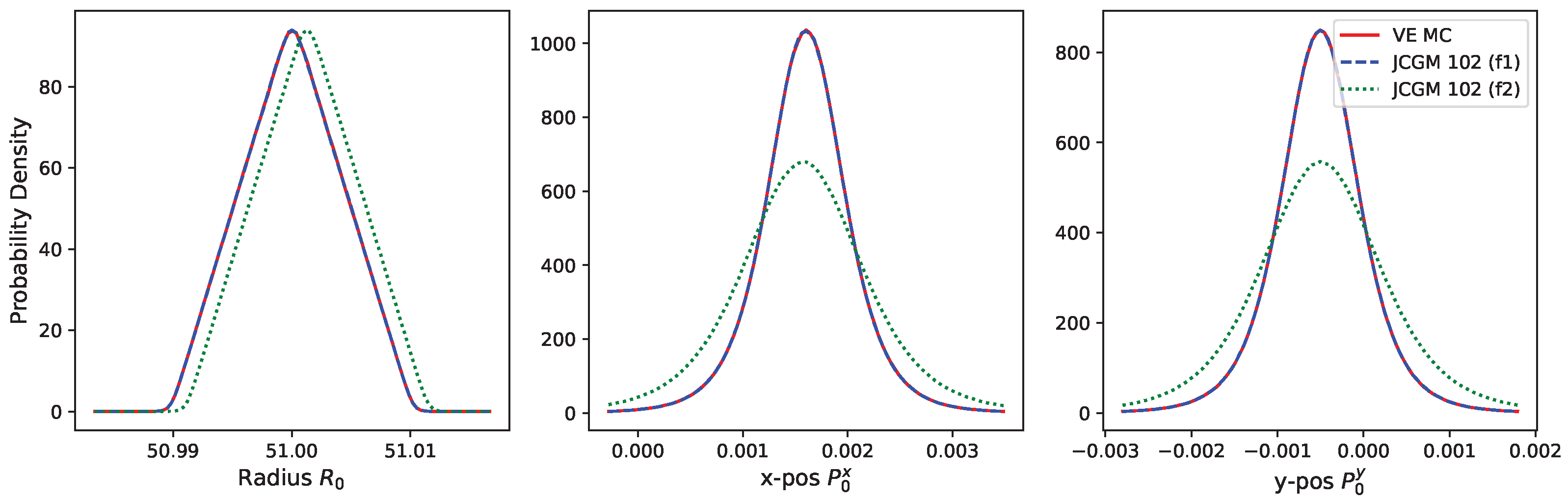
4.2. Coordinate Measuring Machine

A realization of the virtual experiment for the coordinate measuring machine, which yields measurements of $L\ge 3$ points on a circle with radius $r_0>0$ and position of its center $p_0=(p_0^x,p_0^y)\in {\mathbb{R}}^2$, can be obtained by the following formula:

$$x_{\mathcal{l}}^{\mathrm{ve}}=p_{\mathcal{l}}^T=A_{\mathcal{l}}(s_q,s_{c,x},s_{c,y})\left[\begin{array}{c}{r}_0\\ p_0^x\\ p_0^y\end{array}\right]+{ϵ}_{\mathcal{l}}=\left[\begin{array}{cc}{s}_{c,x}& s_q{s}_{c,y}\\ 0& s_{c,y}\end{array}\right]\left[\begin{array}{ccc}cos\left(2\pi \right(\mathcal{l}-1)/L)& 1& 0\\ sin\left(2\pi \right(\mathcal{l}-1)/L& 0& 1\end{array}\right]\left[\begin{array}{c}{r}_0\\ p_0^x\\ p_0^y\end{array}\right]+{ϵ}_{\mathcal{l}},$$

(14)

with $\mathcal{l}=1,\dots ,L$ denoting the L points with assumed noise ${ϵ}_{\mathcal{l}}\sim N(0,{\sigma }^{2}I)$ having specified standard deviation $\sigma >0$. By $s_q$, we denote an angular offset with respect to 90 degrees between the x-axis and y-axis of the coordinate measuring machine, and $s_{c,x}$ and $s_{c,y}$ are scaling factors of the corresponding axis. For this example, we have the dimension of the measured quantity $X=P=(P_1,\dots ,P_L)$ given by $n=2L$ and the measurand $Y=[R,P_0^x,P_0^y]$ has dimension $p=3$. Since this virtual experiment model fits into the general structure of (1) with $B\equiv 0$ and the matrix $A(s_q,s_{c,x},s_{c,y})$ as given in (14), Algorithm 2 can be applied. For this example, Algorithm 2 assumes that the measurement model corresponds to the application of the least-squares fit

$${\left[R_0,P_0^x,P_0^y\right]}^T=f_1(P,S_q,S_{c,x},S_{c,y})=\underset{R,P^x,P^y}{arg\; min}\sum _{\mathcal{l}=1}^L{∥A_{\mathcal{l}}(S_q,S_{c,x},S_{c,y}){\left[R,P^x,P^y\right]}^T-X_{\mathcal{l}}∥}^2,$$

(15)

where $\parallel ·\parallel$ denotes the Euclidean norm, and where we denote the quantities corresponding to the radius, position, squareness and scaling, and the measurements by upper-case letters. This measurement model assumes that the measurement directions are known, i.e., the points $p_{\mathcal{l}}$ are not arbitrarily positioned on the circle but positioned according to the design in (14). Then, the developed Monte Carlo Algorithm 2 yields samples from the same PDF as the application of JCGM-102 and Algorithm 1.

For the coordinate measuring machine, another commonly considered measurement model for this application [32] is the fit of a circle using the circle formula $R^2={(P^x-P_0^x)}^2+{(P^y-P_0^y)}^2$, which can be reformulated in a similar system of equations to (15) using the corrected data points

$${\tilde{P}}_{\mathcal{l}}={\left[\begin{array}{cc}{s}_{c,x}& s_q{s}_{c,y}\\ 0& s_{c,y}\end{array}\right]}^{-1}{P}_{\mathcal{l}},\mathcal{l}=1,\dots ,L$$

(16)

and solving the least-squares problem

$$\left[\begin{array}{c}\tilde{a}\\ \tilde{b}\\ \tilde{c}\end{array}\right]=\underset{a,b,c}{arg\; min}\sum _{\mathcal{l}=1}^L{∥\left[\begin{array}{ccc}{\tilde{P}}_1^x& {\tilde{P}}_1^y& 1\\ & ⋮& \\ {\tilde{P}}_L^x& {\tilde{P}}_L^y& 1\end{array}\right]\left[\begin{array}{c}a\\ b\\ c\end{array}\right]-\left[\begin{array}{c}{\left({\tilde{P}}_1^x\right)}^2+{\left({\tilde{P}}_1^y\right)}^2\\ ⋮\\ {\left({\tilde{P}}_L^x\right)}^2+{\left({\tilde{P}}_L^y\right)}^2\end{array}\right]∥}^2.$$

(17)

yields a vector from which the desired quantities can be derived using

$$R={\displaystyle \frac{1}{2}}\sqrt{4\tilde{c}+{\tilde{a}}^2+{\tilde{b}}^2},P_0^x={\displaystyle \frac{\tilde{a}}{2}},P_0^y={\displaystyle \frac{\tilde{b}}{2}}.$$

(18)

Note that this procedure is equivalent [33] to the solution of the circle fit problem

$${\left[R_0,P_0^x,P_0^y\right]}^T=f_2(P,S_q,S_{c,x},S_{c,y})=\underset{R,P^x,P^y}{arg\; min}\sum _{\mathcal{l}=1}^L{\left|R^2-{∥{\left[\begin{array}{cc}{S}_{c,x}& S_q{S}_{c,y}\\ 0& S_{c,y}\end{array}\right]}^{-1}{P}_{\mathcal{l}}-{\left[P^x,P^y\right]}^T∥}^2\right|}^2,$$

(19)

but does not require the use of a non-linear optimization procedure. In the following, we denote the measurement model that yields the quantities (19) by $f_2$. It can be seen immediately that $f_2$ is a non-linear function in the measured quantity $X=P$. Hence, the application of Algorithm 2 using the virtual experiment (14) will only yield an approximation to the JCGM-102 procedure using the measurement model $f_2$.

For this experiment, we consider a circle with radius of 51 mm centered at $(0.0015,$$-0.00048)$ mm. Then, we generate $m=55$ measurements of $L=25$ equidistant points on the circle boundary, which are disturbed by a squareness effect between the x- and y-axis of $0.0001$ degree and we scale the x-axis by a factor of $0.99$ and the y-axis by a factor of $1.01$. Additionally, independent homoscedastic Gaussian noise with standard deviation $\sigma =0.005$ mm is added to each measurement. From these measurements, the resulting state-of-knowledge PDFs for the measurand, consisting of the radius and position of the circle, can be estimated using the described algorithms, and the resulting marginal PDFs are given in Figure 3. For the Monte Carlo computations, we use $N={10}^5$ samples, and it can be seen that the results of the virtual experiment approach of Algorithm 2, denoted by VEMC, yield the same marginal PDFs as the JCGM-102 approach using the equivalent, linear measurement model $f_1$. For the alternative measurement model $f_2$, the resulting PDFs deviate, both in the position of the mode and the spread of the PDFs.

For a quantitative assessment, we also include the mean estimate, the standard uncertainty, and a 95% coverage interval of the two equivalent approaches in

Table 3. For the coordinate measuring machine example, the resulting estimates in terms of the mean, the standard uncertainty, i.e., standard deviation, and a shortest 95% coverage interval of the marginal distributions are shown for the two approaches using the measurement model (15). All values are given in mm.

Quantity	Mean	Std. Unc.	CI (95%)
Virtual Experiment approach
R	51.0000	0.0042	[50.9920, 51.0080]
$P_0^x$	0.0016	0.0005	[0.0007, 0.0026]
$P_0^y$	−0.0005	0.0006	[−0.0017, 0.0006]
JCGM-102 Monte Carlo approach using (15)
R	51.0000	0.0042	[50.9920, 51.0080]
$P_0^x$	0.0016	0.0005	[0.0007, 0.0025]
$P_0^y$	−0.0005	0.0006	[−0.0017, 0.0006]

and of the JCGM-102 approach using the alternative measurement model in

Table 4. For the coordinate measuring example, the resulting estimates in terms of the mean, the standard uncertainty, i.e., standard deviation, and a shortest 95% coverage interval of the marginal distributions are shown for the JCGM-102 Monte Carlo approach using the measurement model (19). All values are given in mm.

Quantity	Mean	Std. Unc.	CI (95%)
JCGM-102 Monte Carlo approach using (19)
R	51.0013	0.0042	[50.9933, 51.0093]
$P_0^x$	0.0016	0.0007	[0.0001, 0.0030]
$P_0^y$	−0.0005	0.0009	[−0.0023, 0.0013]

. For the approaches corresponding to the measurement model $f_1$ from (15), both Monte Carlo sampling approaches yield the same estimates, standard uncertainties, and coverage intervals. However, for the JCGM-102 approach using the measurement model $f_2$ from (19), the results differ.

5. Conclusions

With this work, we aimed to draw attention to the question of whether an uncertainty evaluation aided by a virtual experiment can be compliant with standards in metrology. For this, we developed a practical relevant approach for an uncertainty evaluation procedure using only realizations of a virtual experiment that yields a PDF that is equivalent to one of these guidelines, the JCGM-102 Monte Carlo approach. In particular, we derived a suitable algorithm that accounts for the a priori unknown variance in the distribution of the observed data, noisy realizations of a virtual experiment, and the sampling procedure is applicable for multivariate data and measurand quantities. We applied this procedure to an example derived from a coordinate measuring machine and have shown that, while the choice of the measurement model matters, equivalent results of a JCGM-102 uncertainty evaluation and the proposed algorithm can be achieved.

With the algorithm derived in this work, an uncertainty evaluation can be performed that is equivalent to a JCGM-102 Monte Carlo sampling procedure. However, we do not require explicit knowledge of the measurement model. This is particularly important when the virtual experiment is highly complex and involves numerical computations that are not easily invertible to infer a measurement model from a virtual experiment.

References

1. Jing, X.; Wang, C.; Pu, G.; Xu, B.; Zhu, S.; Dong, S. Evaluation of measurement uncertainties of virtual instruments. Int. J. Adv. Manuf. Technol. 2006, 27, 1202–1210. [Google Scholar] [CrossRef]
2. ISO-30173:2023; Digital Twin—Concepts and Terminology. International Standard; International Organization for Standardization: Geneva, Switzerland, 2023.
3. Wright, L.; Davidson, S. Digital twins for metrology; metrology for digital twins. Meas. Sci. Technol. 2024, 35, 051001. [Google Scholar] [CrossRef]
4. Irikura, K.K.; Johnson, R.D., III; Kacker, R.N. Uncertainty associated with virtual measurements from computational quantum chemistry models. Metrologia 2004, 41, 369. [Google Scholar] [CrossRef]
5. Trenk, M.; Franke, M.; Schwenke, H. The “Virtual CMM” a software tool for uncertainty evaluation–practical application in an accredited calibration lab. Proc. ASPE Uncertain. Anal. Meas. Des. 2004, 9, 68–75. [Google Scholar]
6. Liu, G.; Xu, Q.; Gao, F.; Guan, Q.; Fang, Q. Analysis of key technologies for virtual instruments metrology. In Fourth International Symposium on Precision Mechanical Measurements; SPIE: Bellingham, WA, USA, 2008; Volume 7130, pp. 1216–1221. [Google Scholar]
7. Heiβelmann, D.; Franke, M.; Rost, K.; Wendt, K.; Kistner, T.; Schwehn, C. Determination of measurement uncertainty by Monte Carlo simulation. In Advanced Mathematical and Computational Tools in Metrology and Testing XI; World Scientific: Singapore, 2019; pp. 192–202. [Google Scholar]
8. Straka, M.; Weissenbrunner, A.; Koglin, C.; Höhne, C.; Schmelter, S. Simulation uncertainty for a virtual ultrasonic flow meter. Metrology 2022, 2, 335–359. [Google Scholar] [CrossRef]
9. Sun, H.; Yang, M.; Wang, H. A virtual experiment for measuring system resilience: A case of chemical process systems. Reliab. Eng. Syst. Saf. 2022, 228, 108829. [Google Scholar] [CrossRef]
10. Balzani, D.; Brands, D.; Schröder, J.; Carstensen, C. Sensitivity analysis of statistical measures for the reconstruction of microstructures based on the minimization of generalized least-square functionals. Tech. Mech.-Eur. J. Eng. Mech. 2010, 30, 297–315. [Google Scholar]
11. Wübbeler, G.; Marschall, M.; Kniel, K.; Heißelmann, D.; Härtig, F.; Elster, C. GUM-compliant uncertainty evaluation using virtual experiments. Metrology 2022, 2, 114–127. [Google Scholar] [CrossRef]
12. Kok, G.; van Dijk, M.; Wübbeler, G.; Elster, C. Virtual experiments for the assessment of data analysis and uncertainty quantification methods in scatterometry. Metrologia 2023, 60, 044001. [Google Scholar] [CrossRef]
13. Kok, G.; Wübbeler, G.; Elster, C. Impact of imperfect artefacts and the modus operandi on uncertainty quantification using virtual instruments. Metrology 2022, 2, 311–319. [Google Scholar] [CrossRef]
14. Hughes, F.; Marschall, M.; Wübbeler, G.; Kok, G.; van Dijk, M.; Elster, C. JCGM 101-compliant uncertainty evaluation using virtual experiments. arXiv 2024, arXiv:2404.10530. In press for XXIV IMEKO World Congress. [Google Scholar]
15. Lira, I.; Wöger, W. Comparison between the conventional and Bayesian approaches to evaluate measurement data. Metrologia 2006, 43, S249. [Google Scholar] [CrossRef]
16. Watzenig, D.; Fox, C. A review of statistical modelling and inference for electrical capacitance tomography. Meas. Sci. Technol. 2009, 20, 052002. [Google Scholar] [CrossRef]
17. Higdon, D.; Gattiker, J.; Williams, B.; Rightley, M. Computer model calibration using high-dimensional output. J. Am. Stat. Assoc. 2008, 103, 570–583. [Google Scholar] [CrossRef]
18. Heidenreich, S.; Gross, H.; Bar, M. Bayesian approach to the statistical inverse problem of scatterometry: Comparison of three surrogate models. Int. J. Uncertain. Quantif. 2015, 5, 511–526. [Google Scholar] [CrossRef]
19. Hammerschmidt, M.; Weiser, M.; Santiago, X.G.; Zschiedrich, L.; Bodermann, B.; Burger, S. Quantifying parameter uncertainties in optical scatterometry using Bayesian inversion. In Modeling Aspects in Optical Metrology VI; SPIE: Bellingham, WA, USA, 2017; Volume 10330, pp. 8–17. [Google Scholar]
20. Kennedy, M.C.; O’Hagan, A. Bayesian calibration of computer models. J. R. Stat. Soc. Ser. B (Stat. Methodol.) 2001, 63, 425–464. [Google Scholar] [CrossRef]
21. Gadd, C.; Xing, W.; Nezhad, M.M.; Shah, A.A. A surrogate modelling approach based on nonlinear dimension reduction for uncertainty quantification in groundwater flow models. Transp. Porous Media 2019, 126, 39–77. [Google Scholar] [CrossRef] [PubMed]
22. Chatterjee, A. An introduction to the proper orthogonal decomposition. Curr. Sci. 2000, 78, 808–817. [Google Scholar]
23. Schwab, C.; Todor, R.A. Karhunen–Loève approximation of random fields by generalized fast multipole methods. J. Comput. Phys. 2006, 217, 100–122. [Google Scholar] [CrossRef]
24. Oseledets, I.V. Tensor-train decomposition. SIAM J. Sci. Comput. 2011, 33, 2295–2317. [Google Scholar] [CrossRef]
25. Balsamo, A.; Di Ciommo, M.; Mugno, R.; Rebaglia, B.; Ricci, E.; Grella, R. Evaluation of CMM uncertainty through Monte Carlo simulations. CIRP Ann. 1999, 48, 425–428. [Google Scholar] [CrossRef]
26. BIPM; IEC; IFCC; ILAC; ISO; IUPAC; IUPAP; OIML. Evaluation of Measurement Data—Supplement 1 to the “Guide to the Expression of Uncertainty in Measurement”—Propagation of Distributions Using a Monte Carlo Method; JCGM 101:2008; Joint Committee for Guides in Metrology: Sèvres, France, 2008. [Google Scholar]
27. BIPM; IEC; IFCC; ILAC; ISO; IUPAC; IUPAP; OIML. Evaluation of Measurement Data—Supplement 2 to the “Guide to the Expression of Uncertainty in Measurement”—Extension to Any Number of Output Quantities; JCGM 102:2011; Joint Committee for Guides in Metrology: Sèvres, France, 2011. [Google Scholar]
28. Kotz, S.; Nadarajah, S. Multivariate t-Distributions and Their Applications; Cambridge University Press: Cambridge, UK, 2004. [Google Scholar]
29. Robert, C.P.; Casella, G.; Casella, G. Monte Carlo Statistical Methods; Springer: New York, NY, USA, 1999; Volume 2. [Google Scholar]
30. Fuller, W.A. Measurement Error Models; John Wiley & Sons: Toronto, ON, Canada, 2009. [Google Scholar]
31. Lira, I.; Grientschnig, D. Error-in-variables models in calibration. Metrologia 2017, 54, S133. [Google Scholar] [CrossRef]
32. Marcel van Dijk, G.K. Comparison of uncertainty evaluation methods for virtual experiments with an application to a virtual CMM. In Proceedings of the XXIV IMEKO World Congress, Hamburg, Germany, 26–29 August 2024. [Google Scholar]
33. Coope, I.D. Circle fitting by linear and nonlinear least squares. J. Optim. Theory Appl. 1993, 76, 381–388. [Google Scholar] [CrossRef]
Figure 1. Experimental setting for the generic polynomial regression example of Section 4.1. The dotted green line indicates the unknown polynomial, from which noisy observations (black crosses) can be conducted at the nominal measurement locations { 1 , , 10 } . The resulting (mean) estimates of the virtual experiment approach (solid red line) and the JCGM-102 Monte Carlo approach (dashed blue line) are shown.
Metrology 04 00033 g001
Figure 2. Marginal densities of the measurand, i.e., polynomial coefficients, of the generic polynomial regression example are shown. The solid red line represents the result of the application of Algorithm 2 using only the virtual experiment and its gradient. The dashed blue line is the result of the JCGM-102 Monte Carlo approach and Algorithm 1 using the corresponding measurement model (13).
Metrology 04 00033 g002
Figure 3. Marginal densities of the measurand, in terms of circle radius and position, of the coordinate measuring machine example are shown. The solid red line represents the result of applying Algorithm 2 using only the virtual experiment and its gradient. The dashed blue line is the result of the JCGM-102 Monte Carlo approach and Algorithm 1 using the corresponding measurement model (15), and the dotted green line corresponds to the JCGM-102 Monte Carlo approach and Algorithm 1 applied to the alternative measurement model (19).
Metrology 04 00033 g003