
GUM-Compliant Uncertainty Evaluation Using Virtual Experiments

 , ,
, ,  , , and
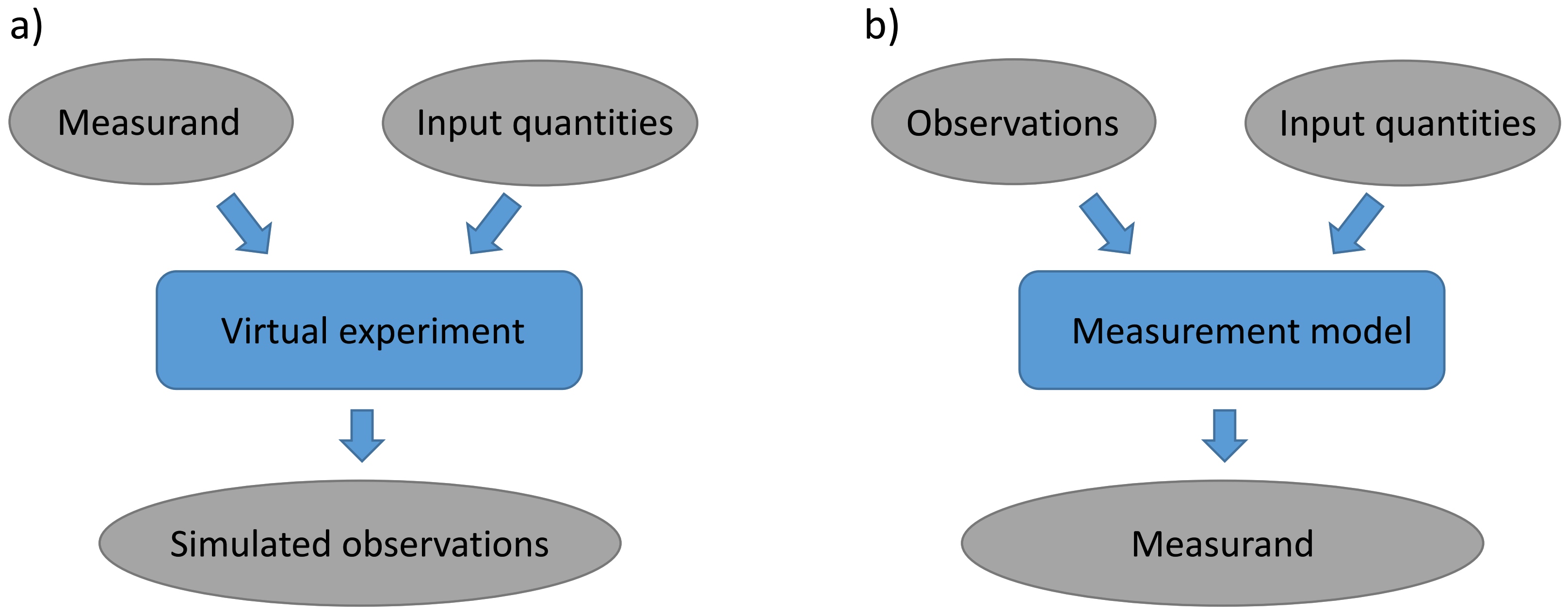
Abstract
:1. Introduction
2. Concepts
2.1. GUM-S1 Monte Carlo Uncertainty Evaluation
- (i)
- Select a at random from the PDF ;
- (ii)
- Select an x at random from the PDF ;
- (iii)
- Calculate .
2.2. Virtual Experiment
- (i)
- Given y, , and ;
- (ii)
- Select an at random from the PDF ;
- (iii)
- Calculate a simulated observation .
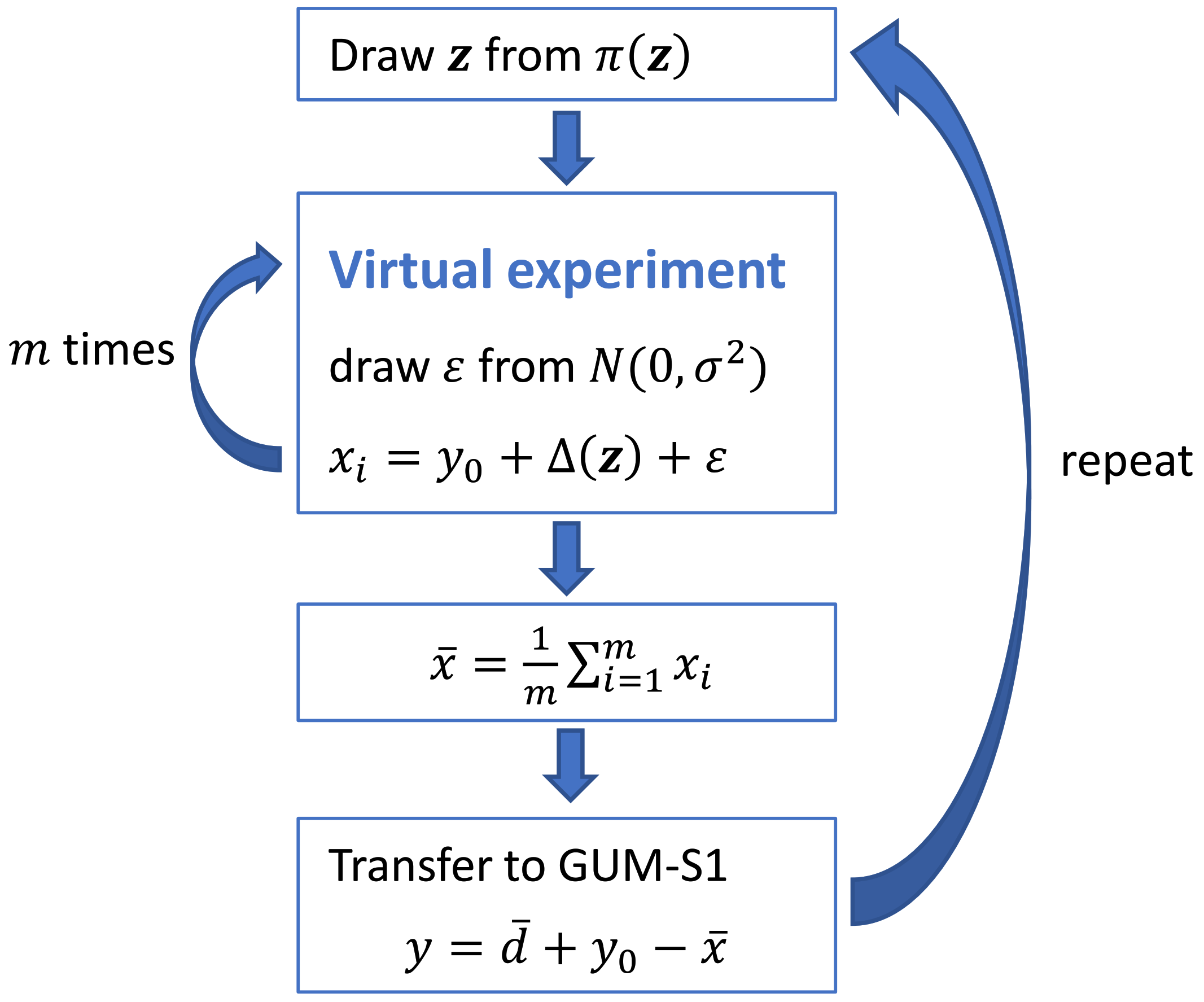
3. GUM-Compliant Uncertainty Evaluation Using Virtual Experiments
3.1. Linear Model and Known Variance
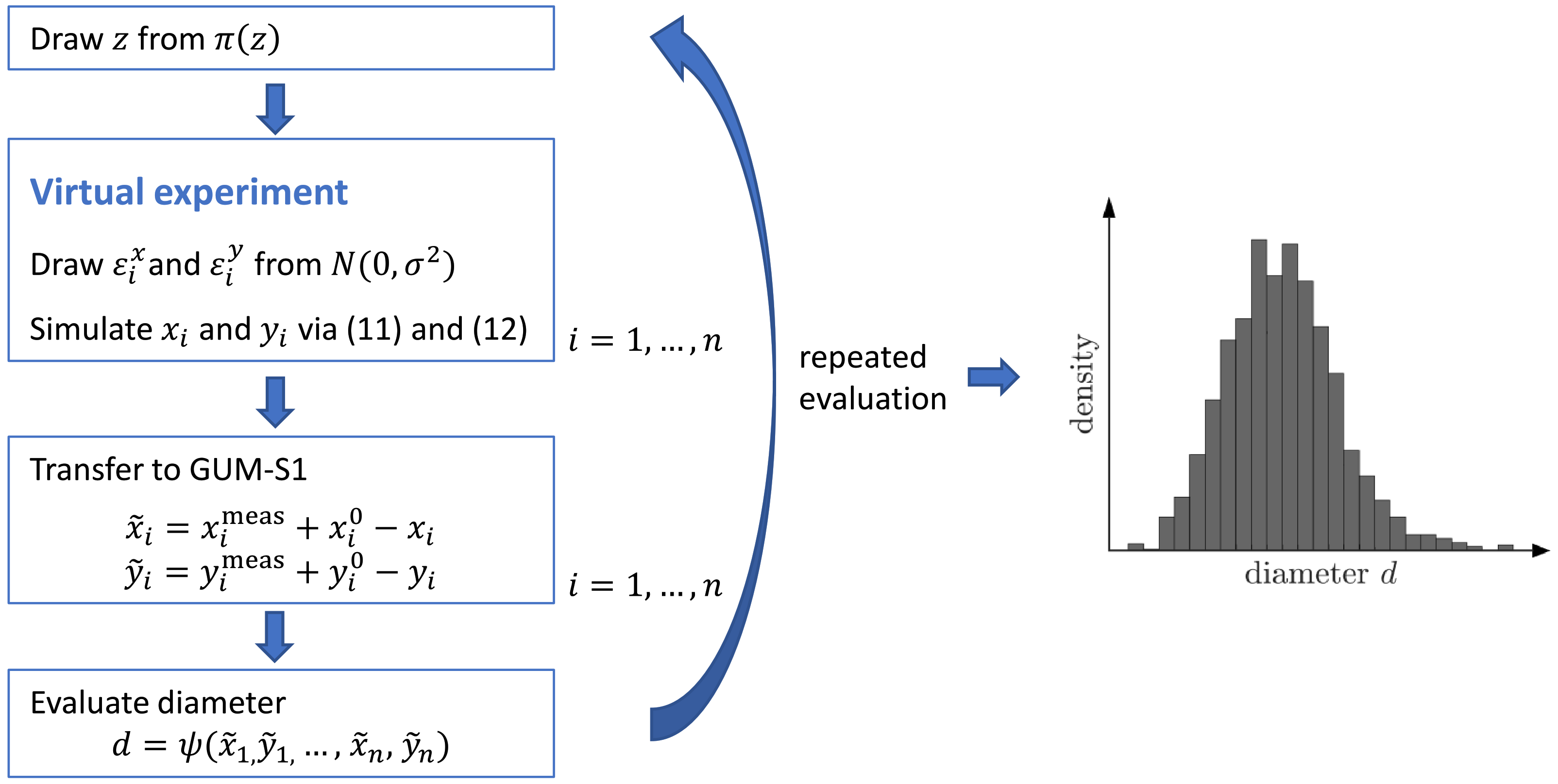
- (i)
- Select a at random from the PDF ;
- (ii)
- Calculate simulated observations through m runs of Virt-Exp for model (3), while using the chosen virtual measurand (and generated in step(i));
- (iii)
- Calculate the mean of the simulated observations ;
- (iv)
- Calculate .
3.2. Linear Model and Unknown Variance
3.3. Nonlinear Model
4. Application
5. Conclusions
Author Contributions
Funding
Institutional Review Board Statement
Informed Consent Statement
Data Availability Statement
Acknowledgments
Conflicts of Interest
References
- Jing, X.; Wang, C.; Pu, G.; Xu, B.; Zhu, S.; Dong, S. Evaluation of measurement uncertainties of virtual instruments. Int. J. Adv. Manuf. Technol. 2006, 27, 1202–1210. [Google Scholar] [CrossRef]
- Irikura, K.K.; Johnson, R.D., III; Kacker, R.N. Uncertainty associated with virtual measurements from computational quantum chemistry models. Metrologia 2004, 41, 369. [Google Scholar] [CrossRef]
- Trenk, M.; Franke, M.; Schwenke, H. The “Virtual CMM” a software tool for uncertainty evaluation—Practical application in an accredited calibration lab. Proc. ASPE Uncertain. Anal. Meas. Des. 2004, 9, 68–75. [Google Scholar]
- Liu, G.; Xu, Q.; Gao, F.; Guan, Q.; Fang, Q. Analysis of key technologies for virtual instruments metrology. In Fourth International Symposium on Precision Mechanical Measurements; International Society for Optics and Photonics: Bellingham, WA, USA, 2008; Volume 7130, p. 71305B. [Google Scholar]
- Doytchinov, I.; Tonnellier, X.; Shore, P.; Nicquevert, B.; Modena, M.; Durand, H.M. Application of probabilistic modelling for the uncertainty evaluation of alignment measurements of large accelerator magnets assemblies. Meas. Sci. Technol. 2018, 29, 054001. [Google Scholar] [CrossRef]
- Heißelmann, D.; Franke, M.; Rost, K.; Wendt, K.; Kistner, T.; Schwehn, C. Determination of measurement uncertainty by Monte Carlo simulation. In Advanced Mathematical and Computational Tools in Metrology and Testing XI; World Scientific: Singapore, 2019; pp. 192–202. [Google Scholar]
- Sepahi-Boroujeni, S.; Mayer, J.; Khameneifar, F. Efficient uncertainty estimation of indirectly measured geometric errors of five-axis machine tools via Monte-Carlo validated GUM framework. Precis. Eng. 2021, 67, 160–171. [Google Scholar] [CrossRef]
- Wiegmann, A.; Stavridis, M.; Walzel, M.; Siewert, F.; Zeschke, T.; Schulz, M.; Elster, C. Accuracy evaluation for sub-aperture interferometry measurements of a synchrotron mirror using virtual experiments. Precis. Eng. 2011, 35, 183–190. [Google Scholar] [CrossRef]
- Balzani, D.; Brands, D.; Schröder, J.; Carstensen, C. Sensitivity analysis of statistical measures for the reconstruction of microstructures based on the minimization of generalized least-square functionals. Tech. Mech. 2010, 30, 297–315. [Google Scholar]
- Fortmeier, I.; Stavridis, M.; Wiegmann, A.; Schulz, M.; Baer, G.; Pruss, C.; Osten, W.; Elster, C. Sensitivity analysis of tilted-wave interferometer asphere measurements using virtual experiments. In Modeling Aspects in Optical Metrology IV; International Society for Optics and Photonics: Bellingham, WA, USA, 2013; Volume 8789, p. 878907. [Google Scholar]
- Trapet, E.; Wäldele, F. The Virtual CMM Concept. In Advanced Mathematical Tools in Metrology; World Scientific: Singapore, 1996; Volume 2, pp. 238–247. [Google Scholar]
- Balsamo, A.; Di Ciommo, M.; Mugno, R.; Rebaglia, B.; Ricci, E.; Grella, R. Evaluation of CMM uncertainty through Monte Carlo simulations. CIRP Ann. 1999, 48, 425–428. [Google Scholar] [CrossRef]
- Aggogeri, F.; Barbato, G.; Barini, E.M.; Genta, G.; Levi, R. Measurement uncertainty assessment of coordinate measuring machines by simulation and planned experimentation. CIRP J. Manuf. Sci. Technol. 2011, 4, 51–56. [Google Scholar] [CrossRef]
- Fortmeier, I.; Stavridis, M.; Wiegmann, A.; Schulz, M.; Osten, W.; Elster, C. Evaluation of absolute form measurements using a tilted-wave interferometer. Opt. Express 2016, 24, 3393–3404. [Google Scholar] [CrossRef] [PubMed]
- Joint Committee for Guides in Metrology. Evaluation of Measurement Data—Guide to the Expression of Uncertainty in Measurement; International Bureau of Weights and Measures (BIPM): Sèvres, France, 2008; BIPM, IEC, IFCC, ILAC, ISO, IUPAC, IUPAP, and OIML, JCGM 100:2008, GUM 1995 with minor corrections. [Google Scholar]
- Joint Committee for Guides in Metrology. Evaluation of Measurement Data—Supplement 1 to the “Guide to the Expression of Uncertainty in Measurement”—Propagation of Distributions Using a Monte Carlo Method; International Bureau of Weights and Measures (BIPM): Sèvres, France, 2008; BIPM, IEC, IFCC, ILAC, ISO, IUPAC, IUPAP, and OIML, JCGM 101: 2008. [Google Scholar]
- Joint Committee for Guides in Metrology. Evaluation of Measurement Data—Supplement 2 to the ‘Guide to the Expression of Uncertainty in Measurement’—Extension to Any Number of Output Quantities; International Bureau of Weights and Measures (BIPM): Sèvres, France, 2011; BIPM, IEC, IFCC, ILAC, ISO, IUPAC, IUPAP, and OIML, JCGM 102: 2011. [Google Scholar]
- Forbes, A.; Sousa, J. The GUM, Bayesian inference and the observation and measurement equations. Measurement 2011, 44, 1422–1435. [Google Scholar] [CrossRef]
- Model, R.; Stosch, R.; Hammerschmidt, U. Virtual experiment design for the transient hot-bridge sensor. Int. J. Thermophys. 2007, 28, 1447–1460. [Google Scholar] [CrossRef]
- Snee, R.D. Validation of regression models: Methods and examples. Technometrics 1977, 19, 415–428. [Google Scholar] [CrossRef]
- Gelman, A.; Meng, X.L.; Stern, H. Posterior predictive assessment of model fitness via realized discrepancies. Stat. Sin. 1996, 6, 733–760. [Google Scholar]
- Jiang, X.; Mahadevan, S. Bayesian risk-based decision method for model validation under uncertainty. Reliab. Eng. Syst. Saf. 2007, 92, 707–718. [Google Scholar] [CrossRef]
- Pawitan, Y. All Likelihood: Statistical Modelling and Inference Using Likelihood; Oxford University Press: Oxford, UK, 2001. [Google Scholar]
- Gelman, A.; Carlin, J.B.; Stern, H.S.; Dunson, D.B.; Vehtari, A.; Rubin, D.B. Bayesian Data Analysis; Chapman and Hall/CRC: London, UK, 2013. [Google Scholar]
- Possolo, A.; Toman, B. Assessment of measurement uncertainty via observation equations. Metrologia 2007, 44, 464. [Google Scholar] [CrossRef]
- Coope, I.D. Circle fitting by linear and nonlinear least squares. J. Optim. Theory. Appl. 1993, 76, 381–388. [Google Scholar] [CrossRef] [Green Version]
- Gander, W.; Golub, G.H.; Strebel, R. Least-squares fitting of circles and ellipses. BIT Numer. Math. 1994, 34, 558–578. [Google Scholar] [CrossRef]


Publisher’s Note: MDPI stays neutral with regard to jurisdictional claims in published maps and institutional affiliations. |
© 2022 by the authors. Licensee MDPI, Basel, Switzerland. This article is an open access article distributed under the terms and conditions of the Creative Commons Attribution (CC BY) license (https://creativecommons.org/licenses/by/4.0/).
Share and Cite
Wübbeler, G.; Marschall, M.; Kniel, K.; Heißelmann, D.; Härtig, F.; Elster, C. GUM-Compliant Uncertainty Evaluation Using Virtual Experiments. Metrology 2022, 2, 114-127. https://doi.org/10.3390/metrology2010008
Wübbeler G, Marschall M, Kniel K, Heißelmann D, Härtig F, Elster C. GUM-Compliant Uncertainty Evaluation Using Virtual Experiments. Metrology. 2022; 2(1):114-127. https://doi.org/10.3390/metrology2010008
Chicago/Turabian StyleWübbeler, Gerd, Manuel Marschall, Karin Kniel, Daniel Heißelmann, Frank Härtig, and Clemens Elster. 2022. "GUM-Compliant Uncertainty Evaluation Using Virtual Experiments" Metrology 2, no. 1: 114-127. https://doi.org/10.3390/metrology2010008
APA StyleWübbeler, G., Marschall, M., Kniel, K., Heißelmann, D., Härtig, F., & Elster, C. (2022). GUM-Compliant Uncertainty Evaluation Using Virtual Experiments. Metrology, 2(1), 114-127. https://doi.org/10.3390/metrology2010008