Noise Limitations in Multi-Fringe Readout of Laser Interferometers and Resonators

Abstract

Laser interferometers that operate over a dynamic range exceeding one wavelength are used as compact displacement sensors for gravitational wave detectors and inertial sensors and in a variety of other high-precision applications. A number of approaches are available to extract the phase from such interferometers by implementing so-called phasemeters, algorithms to provide a linearised phase estimate. While many noise sources have to be considered for any given scheme, they are fundamentally limited by additive noise in the readout, such as electronic readout, digitisation, and shot-noise, which manifest as an effective, white phase noise in the phasemeter output. We calculated and compared the Cramer–Rao lower bound for phasemeters of some state-of-the-art two-beam interferometer schemes and derived their noise limitations for sub-fringe operation and for multi-fringe readout schemes. From this, we derived achievable noise performance levels for one of these interferometer techniques, deep-frequency modulation interferometry. We then applied our analysis to optical resonators and show that frequency scanning techniques can in theory benefit from such resonant enhancement, indicating that the sensitivities can be improved in future sensors.

1. Introduction

Laser interferometers are used for ultra-precise displacement measurements. Gravitational wave detectors are prominent examples, achieving noise levels in the readout of the relative path length changes of ≈${10}^{-19}\mathrm{m}/\sqrt{\mathrm{Hz}}$ [1]. Such levels of precision are achieved using optical wavelengths of about 1 μm by making use of resonant enhancement [2], which is realised by locking the homodyne interferometers to a fixed operating point, limiting their dynamic range to a “sub-fringe” readout.

Interferometer techniques that can provide a much larger dynamic range extending over several wavelengths, so-called “multi-fringe” readout, are studied for applications in which the path length cannot be stabilised. A prominent example is two-beam heterodyne interferometry as used in the space-based gravitational wave detector LISA [3] and its precursor mission LISA Pathfinder [4]. These techniques have demonstrated sensitivities in the range of ≈${10}^{-14}\mathrm{m}/\sqrt{\mathrm{Hz}}$. A number of applications, such as the readout of inertial sensors [5], can benefit from such levels of precision and dynamic range, especially if multiple displacement sensors can be realised with minimal effort, cost, and size. This has caused increased interest and study of techniques such as “quadrature” and “deep-frequency-modulated” interferometers [6]. “Homodyne quadrature interferometers” (HoQI) utilise the polarisation of the light to extend the dynamic range of homodyne interferometers by adding a phase shift to one of the two polarisations, enabling a multi-fringe readout [7]. “Deep-frequency-modulated” (DFM) interferometers aim to combine the multi-fringe capabilities of heterodyne readout with a simplified optical setup [8], thus also increasing the operating range of the interferometer.

It is understood that multi-fringe-capable interferometers cannot reach the same levels of precision as locked homodyne interferometers. The two major reasons for this are the need to readout and digitise a whole interferometric fringe, which limits the optimisation of the readout electronics and comes with a shot-noise penalty, and an incompatibility with resonant enhancement using optical cavities that usually require one to limit the operating range of the interferometer by stabilising the motion of the test masses. Locking the laser frequency to the length of an optical cavity with a test mass motion larger than one wavelength can also reveal the displacement with very high precision, but it requires a dedicated laser source (or actuator) for the readout of each length and hence is not discussed here in the context of techniques studied to realise multiple sensors.

Most of the herein-analysed interferometer types are widely used, and their precision has been measured in various experimental setups. However, a rigorous analysis of their theoretical precision limits has not been performed for all of these interferometer types, meaning it is unclear if the previously reached precision limits are due to experiment-specific conditions or are a more fundamental limit of the used interferometer type such that a different type could archieve a higher precision using the same equipment and surrounding conditions. Specifically for frequency-modulated interferometer setups, which employ a complex readout scheme to decode the phase information from the measured current from the photo diodes, it is important to understand if the precision could be improved by a better readout algorithm (phase estimator) or electronic readout hardware or if the readout functions perfectly and the reached precision is limited by other noise sources.

To answer these questions, we applied the Cramer–Rao lower bound (CRLB) from statistical analysis as the lower limit for an estimator (specifically: the phase estimate). With it, we compared the different interferometer types and their performances under the influence of different noise sources that can be modelled as additive, white noise. Using our analysis, we also found that a new interferometer type has the potential to achieve even higher levels of phase readout precision.

In Section 2, we briefly introduce four interferometer concepts that make use of the interference between two laser beams, and we summarise their specific signal output. Section 3 introduces the Cramer–Rao lower bound as the fundamental limit of the readout and compares this readout limit for the different interferometer types and noise sources that we describe with a common readout noise model. Based on this analysis, we translated, in Section 4, the corresponding readout noise limitations into power spectral densities of the readout displacement noise and present some example noise budgets for future implementations of deep-frequency modulation.

In Section 5, we go beyond two-beam interferometers and analyse the readout noise limits when combining frequency scanning with an optical resonator, suggesting that one can combine signal enhancement with multi-fringe operation. In this context, we show that such a combination can indeed be beneficial to improve the precision levels in future sensors even further.

In Section 6, we conclude and provide an outlook to the development of future sensors with even higher precision.

2. The Interferometer Response, Detection, and Phase Estimation

In this section, we introduce three different multi-fringe interferometers (being capable of measuring distances over multiple fringes/wavelengths), as well as a homodyne interferometer that acts as a baseline precision reference. Each interferometer type sketched here has a topology that captures all of the incoming light power $P_0$, to enable a direct comparison of their shot-noise sensitivity. Each interferometer type also provides at least two complementary output ports. The influence of using only one or both of these ports to estimate the phase is part of our analysis. The interferometric contrast $\kappa$ encompasses mode-mismatching and polarisation-mismatching effects.

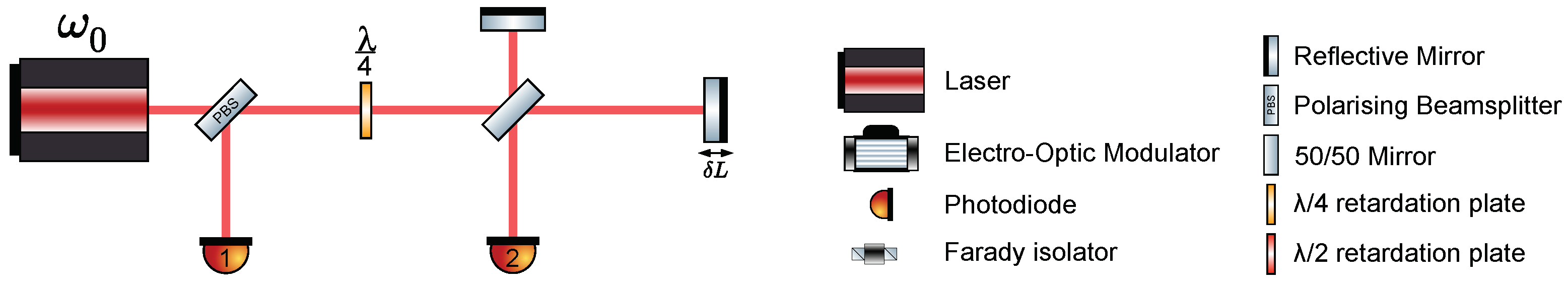
2.1. Homodyne Interferometers

The two output signals of a simple homodyne interferometer, shown in Figure 1, can be written as:

$$\begin{array}{cc}\hfill P_{\mathrm{hom},1}(t,\phi )& \hfill =\frac{P_0}{2}\left(1-\kappa cos\phi \right)\hfill \end{array}$$

(1)

$$\begin{array}{cc}\hfill P_{\mathrm{hom},2}(t,\phi )& \hfill =\frac{P_0}{2}\left(1+\kappa cos\phi \right).\hfill \end{array}$$

(2)

Here, $\phi$ is the interferometric phase, the quantity of interest. The simplest method to extract the phase in a homodyne scheme, which shall be analysed here, is to operate the interferometer at a fixed point on the phase response.

For sufficiently small deviations around the operating point, the change in power is then proportional to the phase change, and realising phase extraction only requires one to calibrate the response and the offset [9].

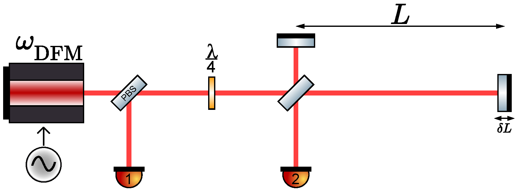
2.2. Heterodyne Interferometer

In a simple heterodyne interferometer, two lasers frequencies are interfered to generate a beat note signal. Figure 2 shows a basic heterodyne setup with the two different frequencies ${\omega }_0$ and ${\omega }_0+\Delta \omega$ present in the setup. Only one of the two laser beams is reflected by the target mirror, while the other goes directly onto the photo diode. The resulting power on the photo diodes is then given by Equations (3) and (4).

$$\begin{array}{cc}\hfill P_{\mathrm{het},1}(t,\phi )& \hfill =\frac{P_0}{2}\left(1-\kappa cos(\Delta \omega t-\phi )\right)\hfill \end{array}$$

(3)

$$\begin{array}{cc}\hfill P_{\mathrm{het},2}(t,\phi )& \hfill =\frac{P_0}{2}\left(1+\kappa cos(\Delta \omega t-\phi )\right)\hfill \end{array}$$

(4)

The measured signal oscillates with the “beat frequency” $\Delta \omega$ over time t, even if there is no phase change ($\delta L=const$). Different schemes are available to extract the phase from the interferometer signals, such as IQ demodulation [10], phase-locked loops [11], or frequency counters [12,13]. The need for a second laser frequency often necessitates setting up a second, stable reference interferometer that enables one to subtract any phase noise in the generation and/or the delivery of the optical signal to the actual interferometer, as performed in LISA Pathfinder [4]. This additional complexity has led to greater interest in schemes that are somewhat simpler, such as the other two described in the following. However, since heterodyne interferometers are well understood and produce highly linearised phase readout, we analysed them here for comparison. In the simplified topology used here, we assumed the existence of a perfect acousto-optic-modulator with a “100%” conversion efficiency, as sketched in Figure 2.

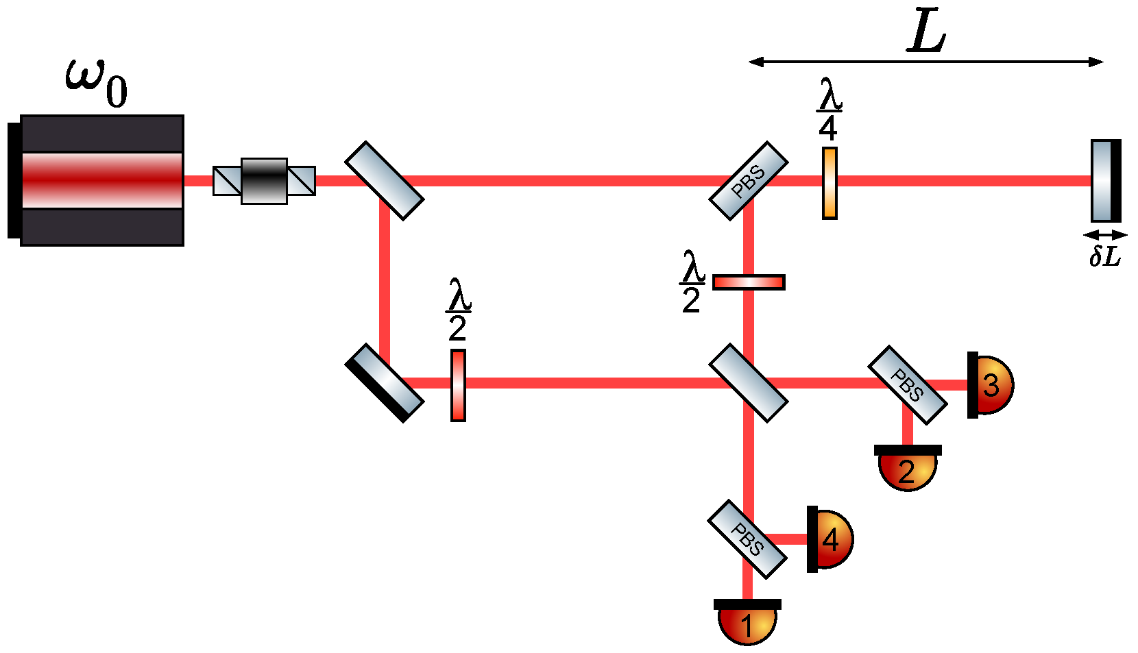
2.3. Homodyne Quadrature Interferometer

Another method to increase the dynamic range of homodyne interferometers by utilizing the polarisation of the light are so-called homodyne quadrature interferometers [7]. A basic setup can be seen in Figure 3. By effectively giving one of two orthogonal polarisations and an additional constant phase shift and using additional photo diodes to measure both polarisations individually, the $2\pi$ ambiguity of the phase readout can be bypassed [6]. The four output port signals of this interferometer are given by:

$$\begin{array}{c}\hfill P_1=\frac{P_0}{4}\left(1+\kappa cos\phi \right)P_2=\frac{P_0}{4}\left(1-\kappa sin\phi \right)\\ \hfill P_3=\frac{P_0}{4}\left(1-\kappa cos\phi \right)P_4=\frac{P_0}{4}\left(1+\kappa sin\phi \right).\end{array}$$

(5)

The phase is extracted elegantly by forming simple linear combinations of the four digitised signals in such a way that the offset terms vanish and quadrature signals are revealed from which the phase can directly be calculated. In our analysis, we treated linear combinations formed by three of the four signals as one phase output (comparable to one photo detector in heterodyne readout), because this is the minimal number of ports required to provide a linear phase estimate. If all four signals were used, we treated this as two (or all) phase output ports being used to achieve minimal readout noise.

2.4. Deep-Frequency-Modulated Interferometry

An alternative scheme to generate heterodyne-like signals is to combine an unequal arm-length homodyne interferometer with a strong, sinusoidal modulation of the laser frequency [14].

The output signals for such an interferometer as seen in Figure 4 can be written as:

$$\begin{array}{cc}\hfill P_{{\mathrm{DFM}}_{1,2}}& \hfill =\frac{P_0}{2}\left(1\mp \kappa cos\left\{msin({\omega }_{m}t+\psi )+\phi \right\}\right)\hfill \end{array}$$

(6)

$$\begin{array}{cc}\hfill & \hfill \mathrm{with}m=\Delta \omega \tau \mathrm{and}\tau =L/c\hfill \end{array}$$

(7)

The effective modulation depth m depends on the arm-length mismatch L, the speed of light c in a vacuum, and the depth of the frequency modulation $\Delta \omega$. Using the Anger–Jacobi identity, this signal can be rewritten as Fourier series with Bessel functions $J_n$ as coefficients, which is usually used for the calculations performed in this article (as in [15]).

$$P_{\mathrm{DFM}}\left(t\right)=\frac{P_0}{2}\left(1\mp \kappa \sum _{n\in \mathbb{Z}}{J}_n\left(m\right)cos(n({\omega }_{m}t+\psi )+\phi )\right)$$

(8)

The phase extraction can be realised using an algorithm originally developed for strong phase modulation interferometers [16]. The basic principle is to demodulate the signal based at multiples of the modulation frequency and then use a fit algorithm to match an analytic model of the signal to these harmonic amplitudes, thereby revealing the desired signal parameters ($\frac{P_0\kappa }{2}$, m, $\psi$, $\phi$). This technique also provides an estimate of the absolute arm-length difference, encoded in the modulation depth m.

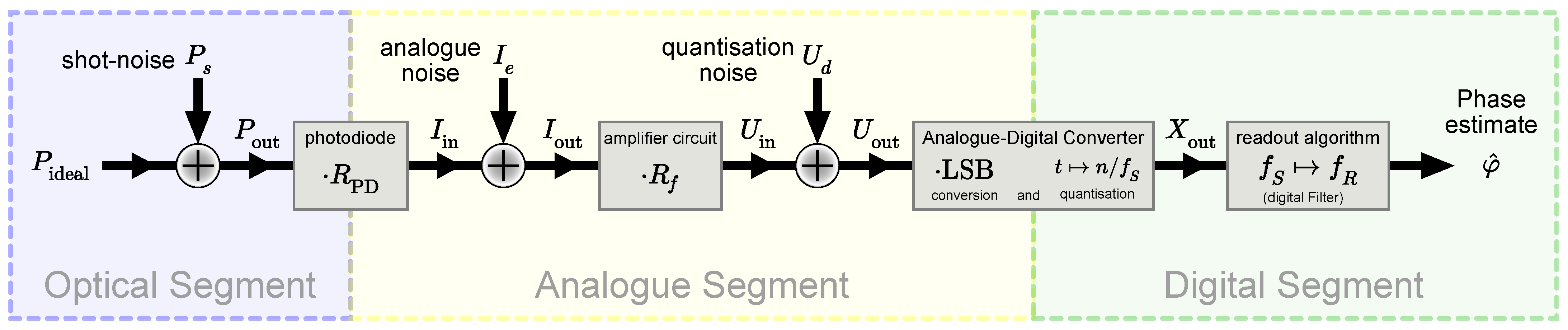
2.5. Common Interferometer Readout Noise Model

We assumed here a common readout chain model for each of the above-listed interferometer types. A block diagram of the model is shown in Figure 5.

Each optical signal contains a shot-noise contribution and is fully collected by a photo diode, which converts the optical power into a current via its responsivity $R_{\mathrm{PD}}=\eta \frac{q\lambda }{hc}$ ($\left[R_{\mathrm{PD}}\right]=A/W$), with $\eta$ as the quantum efficiency, $\lambda$ as the optical wavelength, and q as the elementary charge. In the following analogue signal chain, various electronic noise sources contribute, which we modelled as an additive, white, Gaussian current noise. The current is converted into a voltage via a trans-impedance amplifier with a gain given by an effective resistance $R_{\mathrm{f}}$ ($\left[R_{\mathrm{f}}\right]=V/A=\mathsf{\Omega }$). The voltage is then digitised by an analogue-to-digital converter. In this process, the digitisation noise is added to the signal, modelled here as an additive voltage noise; the signal is sampled at frequency $f_S$, and it is converted into a unit-less number by division with the “least significant bit” (LSB), which is defined by the ADC voltage input range $\Delta V_{\mathrm{ADC}}$ and the number of bits NOB:

$$\mathrm{LSB}=\frac{\Delta V_{\mathrm{ADC}}}{2^{\mathrm{NOB}}}$$

(9)

These digital values, $X_{\mathrm{out}}$, are then used in the phase extraction algorithms to estimate the interferometric phase $\widehat{\phi }$. The results of the algorithms are then generally provided at an equal or lower rate, the readout rate $f_R\le f_S$, and we assumed both for the initial digitisation and the decimation to $f_R$ that sufficient filtering was applied to avoid aliasing effects, containing the remaining noise fully within the respective Nyquist frequencies of $f_S/2$ and $f_R/2$, respectively.

For convenience, we also introduce the ADC “fill-factor”:

$$\alpha =\frac{V_0}{\Delta V_{\mathrm{ADC}}}=\frac{R_{\mathrm{PD}}{R}_f\kappa P_0}{\Delta V_{\mathrm{ADC}}}$$

(10)

as the ratio between the maximal voltage of each optical signal and the ADC’s full voltage range.

In Figure 6, we sketch the optical signals, noise, and sampling/readout frequencies for the discussed interferometer types. In the case of homodyne and quadrature interferometers, the optical signals are directly in the measurement band and at the same frequency of the phase signals. For heterodyne and DFM interferometers, the optical signals are at higher frequencies, which are typically within the sampling bandwidth and above the readout and phase signal bandwidth. Here, we treated all noise contributions as white noise to compare the different schemes. For digitisation and shot-noise, this is appropriate, but in the case of electronic noise, this is a strong simplification. The impact of this simplification depends on the readout scheme. For homodyne and quadrature readout, one should expect a significant low-frequency electronic noise increase by 1/f-type contributions that will couple into the phase readout. We discard this effect for now and address it later in Section 4 and Section 5. For heterodyne and DFM readout, 1/f-type electronic noise contributions are present as well, but here, only the noise level at the signal frequencies matters for our calculations. Therefore, we accounted for this effect by assuming an effective white noise level at the respective electronic signal frequencies.

3. The Cramer–Rao Lower Bound of the Readout

In order to quantify the fundamental limits of the phase estimation, we used the Cramer–Rao lower bound, which reveals the lower limit of the phase estimation independent of the specific readout algorithm. The CRLB is calculated from the probability distribution of the measured signal $X_{\mathrm{out}}$. This probability distribution in turn depends on the ideal signal $P_{\mathrm{ideal}}$ and the different noise distributions.

In the following discussion, we consider three different, additive noise contributions, each with a specific distribution: shot-noise is caused by a Poisson distribution; electronic noise is modelled by a Gaussian distribution; quantisation noise is ideally modelled with a uniform distribution. Assuming a linear chain of conversion in the readout chain, we can write the measured signal as:

$$X_{\mathrm{out}}(t,\phi )=\frac{R_{\mathrm{PD}}{R}_f}{\mathrm{LSB}}{P}_{\mathrm{ideal}}(t,\phi )+\frac{R_{\mathrm{PD}}{R}_f}{\mathrm{LSB}}{P}_s(t,\phi )+\frac{R_f}{\mathrm{LSB}}{I}_e+\frac{1}{\mathrm{LSB}}{U}_d.$$

(11)

We describe all of these noise influences as band-limited white noise, which assumes that the laser is shot-noise limited in the frequency band of interest. The CRLB for the variance of the estimator $\widehat{\phi }$ for $\phi$ is given by:

$$\mathrm{var}\left(\widehat{\phi }\right)\ge \frac{1}{\mathbb{E}\left[{\left(\frac{\partial (ln\rho (x;\phi \left)\right)}{\partial \phi }\right)}^2\right]}=\frac{1}{\mathrm{FI}\left(\phi \right)}$$

(12)

with $\mathrm{var}\left(\widehat{\phi }\right)$ as the variance of $\widehat{\phi }$, $\rho$ as the probability density function of the random variable X, $\mathbb{E}[·]$ as the expectation value, and $\mathrm{FI}\left(\phi \right)$ as the “Fisher information” [17] (Chapter 4).

For the case of measuring multiple interferometer outputs (since every interferometer has at least two optical outputs) with uncorrelated noise, we made use of the fact that the Fisher information of two independent random variables $P_1$ and $P_2$ is simply the sum of the Fisher information of the individual outputs. We used the same argument to study the combined influence of the three uncorrelated noise sources in the readout chain.

3.1. Different Noise Sources and Their Lower Bound

3.1.1. The CRLB of Shot-Noise (Poisson Distribution)

We describe the shot-noise by a Poisson distribution for the number of electrons N that are measured during the sampling time $1/f_S$ on the photo diode, given by:

$$\rho \left(N\right)=\frac{e^{-N_0}{N}_0^N}{N!}$$

(13)

where $N(t,\phi )=P_{\mathrm{out}}(t,\phi )·\eta /\hslash \omega f_S$ would be the measured (noisy) electron number (over the time period $1/f_S$) and $N_0(t,\phi )=P_{\mathrm{ideal}}(t,\phi )·\eta /\hslash \omega f_S$ the ideal (mean) electron number of the signal (with $\eta$ as the quantum efficiency of the photo diode).

Plugging the resulting probability distribution:

$$\rho \left(P_{\mathrm{out}}\right)=\frac{e^{-\frac{\eta P_{\mathrm{ideal}}}{\hslash \omega f_S}}{\left(\frac{\eta P_{\mathrm{ideal}}}{\hslash \omega f_S}\right)}^{\left(\frac{\eta P_{\mathrm{out}}}{\hslash \omega f_S}\right)}}{\left(\frac{\eta P_{\mathrm{out}}}{\hslash \omega f_S}\right)!}$$

(14)

into (12) (as performed in [15]) leads to a CRLB of:

$$\mathrm{var}\left({\widehat{\phi }}_{\mathrm{shot}}\right)\ge \frac{\hslash \omega }{\eta }·\frac{1}{{\int }_0^T\frac{{\left(\frac{\partial P_{\mathrm{ideal}}(t,\phi )}{\partial \phi }\right)}^2}{P_{\mathrm{ideal}}(t,\phi )}dt}$$

(15)

3.1.2. The CRLB for Electronic (Gaussian) Noise

The electronic noise contribution can be written as:

$$I_{\mathrm{out}}(t,\phi )=I_{\mathrm{in}}(t,\phi )+I_e$$

(16)

The probability distribution of the Gaussian noise $I_e$ was set to be:

$$\rho \left(I_e\right)=\frac{1}{\sqrt{2\pi }\sigma }exp\left(-\frac{I_e^2}{2{\sigma }^2}\right)$$

(17)

with ${\sigma }^2=f_S·S_{II}=f_S·({\tilde{I}}_e^2/2)$ as the variance, $S_{II}$ as the double-sided power spectral density of the current noise, and ${\tilde{I}}_e$ as the single-sided amplitude spectral density. (Here, $I_{\mathrm{out}},I_{\mathrm{in}},I_e$, and $\sigma$ would be given in units of Amperes). The resulting probability distribution for the measured signal is then:

$$\rho \left(I_{\mathrm{out}}\right)=\frac{1}{\sqrt{2\pi }\sigma }exp\left(-\frac{{\left(I_{\mathrm{out}}-I_{\mathrm{in}}\right)}^2}{2{\sigma }^2}\right)$$

(18)

Plugging this probability distribution into (12) allows us to calculate the CRLB. Reference [15] went into detail about the individual steps of the calculation for the CRLB of a finite measurement period T (using $N=f_{S}T$ data points). With an approximation for a large sampling frequency, the resulting CRLB is given by:

$$\mathrm{var}\left(\widehat{\phi }\right)\ge \frac{{\sigma }^2}{f_S{\int }_0^{T}dt{\left(\frac{\partial I_{\mathrm{in}}(t,\phi )}{\partial \phi }\right)}^2}=\frac{{\tilde{I}}_e^2}{2{\int }_0^{T}dt{\left(\frac{\partial I_{\mathrm{in}}(t,\phi )}{\partial \phi }\right)}^2}$$

(19)

3.1.3. The Digitisation Noise (Uniform Distribution)

Digitisation noise has a uniform distribution, but it fails the Cramer–Rao regularity conditions [17] (Section 4.3) at its edges, meaning that the Cramer–Rao inequality cannot be applied for a (purely) uniform distributions. A common practice is to approximate the uniform quantisation noise by a Gaussian with the same variance of ${\sigma }^2={\mathrm{LSB}}^2/12$.

$$U_{\mathrm{out}}\left(t_n\right)=U_{\mathrm{in}}(t_n=n/f_S)+U_d\mathrm{with}n\in \mathbb{N}$$

(20)

The approximate distribution of the quantisation noise would then be given by:

$$\rho \left(U_{\mathrm{out}}\right)\approx \frac{1}{\sqrt{2\pi \frac{{\mathrm{LSB}}^2}{12}}}exp\left(-\frac{{\left(U_{\mathrm{out}}-U_{\mathrm{in}}\right)}^2}{2\frac{{\mathrm{LSB}}^2}{12}}\right)$$

(21)

which would lead to a similar CRLB as before:

$$\mathrm{var}\left(\widehat{\phi }\right)\ge \frac{\frac{{\mathrm{LSB}}^2}{12}}{f_S{\int }_0^{T}dt{\left(\frac{\partial U_{\mathrm{in}}(t,\phi )}{\partial \phi }\right)}^2}$$

(22)

3.2. Comparison of CRLB Limitations for Different Interferometer Types

With the previously introduced formulas for the limit of the readout for different noise distributions, we can now calculate the readout limits for each noise source (Equations (15), (19), and (22)), for the four different interferometer types (Equations (2) and (4)–(6)) and find analytic solutions. We calculated the variance of the phase estimator from a sample measurement of size $N=f_S/f_R$ data points that accounts for the varying size of each variance depending on the readout rate. The results of these calculations are displayed in

Table 1. Comparison of the Cramer–Rao lower bound for different interferometer types with the same laser power. The ± signs correspond to the different measurable outputs of the interferometer setup. For the quadrature setup, “single output” refers to using and digitising three optical signal to form the linear readout combinations.

$\mathbf{var}\left(\widehat{\mathit{\phi }}\right)$≥	Single Output	Combined Output
hom.	$\frac{2}{1\pm cos\phi }{\sigma }_{\mathrm{s}}^2+\frac{8}{1-cos2\phi }({\sigma }_{\mathrm{e}}^2+{\sigma }_{\mathrm{d}}^2)$	$1{\sigma }_{\mathrm{s}}^2+\frac{4}{1-cos2\phi }({\sigma }_{\mathrm{e}}^2+{\sigma }_{\mathrm{d}}^2)$
het.	$2{\sigma }_{\mathrm{s}}^2+8({\sigma }_{\mathrm{e}}^2+{\sigma }_{\mathrm{d}}^2)$	$1{\sigma }_{\mathrm{s}}^2+4({\sigma }_{\mathrm{e}}^2+{\sigma }_{\mathrm{d}}^2)$
quad.	$2{\sigma }_{\mathrm{s}}^2+16({\sigma }_{\mathrm{e}}^2+{\sigma }_{\mathrm{d}}^2)$	$1{\sigma }_{\mathrm{s}}^2+8({\sigma }_{\mathrm{e}}^2+{\sigma }_{\mathrm{d}}^2)$
DFMI	$\frac{2}{1\pm J_0\left(m\right)·cos\phi }{\sigma }_{\mathrm{s}}^2+\frac{8}{1-J_0\left(2m\right)·cos2\phi }({\sigma }_{\mathrm{e}}^2+{\sigma }_{\mathrm{d}}^2)$	$1{\sigma }_{\mathrm{s}}^2+\frac{4}{1-J_0\left(2m\right)·cos2\phi }({\sigma }_{\mathrm{e}}^2+{\sigma }_{\mathrm{d}}^2)$

, with the constants ${\sigma }_{\mathrm{s}}^2$, ${\sigma }_{\mathrm{e}}^2$, and ${\sigma }_{\mathrm{d}}^2$ as factors for shot-noise, electronic noise, and digitisation noise given by:

$${\sigma }_{\mathrm{s}}^2=\frac{f_R\hslash {\omega }_0}{\kappa \eta P_0},{\sigma }_{\mathrm{e}}^2=\frac{f_R{\tilde{I}}_e^2}{2R_{\mathrm{PD}}^2{\kappa }^2{P}_0^2}\mathrm{and}{\sigma }_{\mathrm{d}}^2=\frac{f_R{\mathrm{LSB}}^2}{12f_S{R}_f^2{R}_{\mathrm{PD}}^2{\kappa }^2{P}_0^2}$$

(23)

In order to calculate the different CRLBs, we conveniently chose the measurement period T to be $=n·2\pi /\Delta \omega$ for the heterodyne setup and $=n·2\pi /\Delta {\omega }_m$ for the DFM setup, with n as the integer. The constant factors in Equation (23) show, as expected, that only the digitisation noise contribution depended on the direct sampling frequency.

The homodyne setup shows the expected dependency on the operating point. For example, close to the dark fringe ($\phi =0$ for one output), the shot-noise becomes minimal because the ratio of the signal derivative ${(\partial P_{\mathrm{ideal}}/\partial \phi )}^2$ to the mean power is maximised, because the latter is minimal. In the case of the optimal, combined readout, the shot-noise is independent of the operating point. The influence of electronic and digitisation noise was minimal at points with a maximal signal derivative.

The heterodyne setup has in contrast no dependency on the operating point. The variances (and readout limit) are independent of the chosen output or any operating point, leading to a fixed readout limit because of the time averaging in the CRLBs, just as expected in the case of a well-defined signal-to-noise ratio.

The quadrature setup has also no dependency on the operating point. While the readout limit for the shot-noise is the same as for the heterodyne case, the readout limit for additive Gaussian noise (electronic and digitisation) is slightly worse by a factor of two ($\sqrt{2}$ in amplitude).

Finally, the DFM readout limit also depends on the operating point, even though it is less significant than in the homodyne setup. Firstly, we see that for a vanishing modulation $m\to 0$, the readout limit converged to the homodyne readout limit ($J_0\left(m\right)\to 1$). For a finite modulation depth m, the dependency on the operating point remains, although to a lesser extent. For large m, the dependency on the operating point can be neglected if both output ports are used and one can achieve the same readout limit as in a heterodyne setup. The dependency on $J_0\left(m\right)$ for shot-noise and a single output can again be understood by the minimisation of the mean power. The dependency on $J_0\left(2m\right)$ for electronic and digitisation noise is similarly driven by the square of the overall slope of the signal within a phase estimation period ($1/f_R$).

4. Readout Limit in the Frequency Domain

We also rewrote these results as power spectral densities of the effective displacement measurement noise to provide a simple basis for calculating such noise budgets and to discuss some specific examples.

For white readout noise, the power spectral density of the phase noise was derived by uniformly distributing the above-calculated CRLB variances on the readout bandwidth:

$${\widehat{S}}_{\phi \phi }\left(f\right)=\frac{1}{f_R}\mathrm{var}\left(\widehat{\phi }\right)\mathrm{for}f\in [-f_R/2,f_R/2].$$

(24)

To convert phase to displacement noise, we took into account that in the herein-studied interferometer topologies, the measurements were performed in reflection, $\delta \widehat{L}=\lambda /4\pi ·\widehat{\phi }$. Accordingly, the power spectral density of the length noise is:

$$2{\widehat{S}}_{\mathrm{L}\mathrm{L}}\left(f\right)=\frac{{\lambda }^2}{{\left(4\pi \right)}^2}\frac{2}{f_R}\mathrm{var}\left(\widehat{\phi }\right)=:{\tilde{L}}^2.$$

(25)

We again define three constants as factors for each noise contribution:

$$\begin{array}{cc}\hfill {\tilde{L}}_{\mathrm{s}}^2=& \hfill \frac{\hslash c\lambda }{4\pi \eta \kappa P_0}=\frac{{\lambda }^2{q}_e}{8{\pi }^2{R}_{\mathrm{PD}}\kappa P_0},{\tilde{L}}_{\mathrm{e}(+)}^2={\left(\frac{{\tilde{I}}_{e(+)}\lambda }{2\pi R_{\mathrm{PD}}\kappa P_0}\right)}^2\hfill \\ \hfill \mathrm{and}{\tilde{L}}_{\mathrm{d}}^2=& {\left(\frac{\lambda 2^{-\mathrm{NOB}}}{2\pi \sqrt{6f_S}\alpha }\right)}^2.\hfill \end{array}$$

(26)

The effective noise power spectra are listed in

Table 2. Comparison of the displacement power spectral density of the Cramer–Rao lower bound for different interferometer types, rewritten from Table 1.

${\tilde{\mathit{L}}}^2$≥	Single Output	Combined Output
hom.	$\frac{2}{1\pm cos\phi }{\tilde{L}}_{\mathrm{s}}^2+\frac{2}{1-cos2\phi }({\tilde{L}}_{\mathrm{e}+}^2+{\tilde{L}}_{\mathrm{d}}^2)$	$1{\tilde{L}}_{\mathrm{s}}^2+\frac{1}{1-cos2\phi }({\tilde{L}}_{\mathrm{e}+}^2+{\tilde{L}}_{\mathrm{d}}^2)$
het.	$2{\tilde{L}}_{\mathrm{s}}^2+2({\tilde{L}}_{\mathrm{e}}^2+{\tilde{L}}_{\mathrm{d}}^2)$	$1{\tilde{L}}_{\mathrm{s}}^2+1({\tilde{L}}_{\mathrm{e}}^2+{\tilde{L}}_{\mathrm{d}}^2)$
quad.	$2{\tilde{L}}_{\mathrm{s}}^2+4({\tilde{L}}_{\mathrm{e}+}^2+{\tilde{L}}_{\mathrm{d}}^2)$	$1{\tilde{L}}_{\mathrm{s}}^2+2({\tilde{L}}_{\mathrm{e}+}^2+{\tilde{L}}_{\mathrm{d}}^2)$
DFMI	$\frac{2}{1\pm J_0\left(m\right)·cos\phi }{\tilde{L}}_{\mathrm{s}}^2+\frac{2}{1-J_0\left(2m\right)·cos2\phi }({\tilde{L}}_{\mathrm{e}}^2+{\tilde{L}}_{\mathrm{d}}^2)$	$1{\tilde{L}}_{\mathrm{s}}^2+\frac{1}{1-J_0\left(2m\right)·cos2\phi }({\tilde{L}}_{\mathrm{e}}^2+{\tilde{L}}_{\mathrm{d}}^2)$

. Table 2 shows the previously calculated CRLB from Table 1 converted to the power spectral density.

Using these results, we can now calculate the fundamental readout noise limitations of each interferometer type that are determined by the readout noise sources. One should note that this calculation does not include other technical noise sources, such as laser amplitude and frequency noise, ADC timing jitter, polarisation effects, ghost beams, and scattered light and other non-linear noise couplings. These effects vary strongly between the different techniques and their implementations and will potentially dominate over the noise limits calculated here if not sufficiently suppressed in the respective sensor design.

One of the limitations that is shared between all multi-fringe techniques is the digitisation noise, which in turn is limited by the available analogue-to-digital converters and their dynamic range with ${\tilde{L}}_d\propto 2^{-\mathrm{NOB}}/\left(\sqrt{f_{\mathrm{S}}}\alpha \right)$ and their need to avoid clipping in the digitisation process ($\alpha \le 1)$). The electronic noise of converters can either be accounted for by projecting it as equivalent input current noise or by instead using their effective number of bits (ENOB), instead of their NOB.

In the case of homodyne and quadrature readout, one should additionally include the earlier mentioned effects of 1/f-type electronic noise. While our calculations did not account for them, the frequency domain noise models we derived equate to the results of linear-time-invariant system models for these DC readout techniques. Effectively, this means that in those cases, one can use the appropriate frequency-dependent noise model ${\tilde{I}}_{e+}$ and obtain the full, frequency-dependent phase/length readout noise contributions. We mark the respective frequency-dependent electronic noise contributions in Table 1 as ${\tilde{L}}_{\mathrm{e}+}$.

For DFMI (with $m\approx 7$ and $J_0\left(2m\right)\approx 0.17$), we calculated the readout noise for two example cases. In both cases, we assumed an optical contrast of $\kappa =90\%$ and an ADC utilisation ratio of $\alpha =90\%$. The assumed parameters and resulting noise levels are shown in

Table 3. Ideal readout noise limits for two different DFMI setups. Shown are the assumed set-up parameters, the individual readout noise contributions, and the resulting total noise. These levels of displacement noise do not take the need for reference measurements, for example to stabilise the laser frequency, into account, but show only the limit for a single interferometer. In the case of the DFMI, a comparison with single reference interferometer would be required, and this would lead to an increase of the total noise by a factor $\sqrt{2}$, if both interferometers have the same readout noise level.

Value	$\mathit{\lambda }$	${\mathit{P}}_0$	${\mathit{f}}_{\mathbf{S}}$	NOB	${\mathit{R}}_{\mathbf{PD}}$	${\tilde{\mathit{I}}}_{\mathit{e}}$	${\tilde{\mathit{L}}}_{\mathbf{s}}$	${\tilde{\mathit{L}}}_{\mathbf{e}}$	${\tilde{\mathit{L}}}_{\mathbf{d}}$	$\tilde{\mathit{L}}$
Unit	nm	mW	MHz	1	A/W	$\frac{\mathbf{pA}}{\sqrt{\mathbf{Hz}}}$	$\frac{\mathbf{fm}}{\sqrt{\mathbf{Hz}}}$	$\frac{\mathbf{fm}}{\sqrt{\mathbf{Hz}}}$	$\frac{\mathbf{fm}}{\sqrt{\mathbf{Hz}}}$	$\frac{\mathbf{fm}}{\sqrt{\mathbf{Hz}}}$
DFMI 1	1550	2	1	15	1.1	30	1.57	≤4.49	≤4.55	≤6.58
DFMI 2	532	10	4	17	0.36	30	0.42	≤0.94	≤0.18	≤1.05

.

The equivalent input current noise dominates in both cases. Lower noise levels can be achieved in photodetectors, but our model also includes the electronic noise of the analogue-to-digital converters and their front-end electronics. For an ADC with a voltage range of 10 V the herein-assumed equivalent input current noise ${\tilde{I}}_e$ corresponds to a voltage noise of ${\tilde{U}}_e=83\frac{nV}{\sqrt{\mathrm{Hz}}}$, which we consider a quite demanding value, especially at typical DFMI optical signal frequencies of 1 kHz to 10 kHz.

The second example is an optimised scenario based on the best available analogue-to-digital converter for this purpose, relatively high input power, and a shorter wavelength that is likely still compatible with typical DFMI optics. The example shows on the one hand that sub-femtometer-level precision is theoretically possible and on the other hand that at least with the assumption used in this analysis, one cannot expect to go much beyond this level of sensitivity. While sensitivities below $10\frac{fm}{\sqrt{\mathrm{Hz}}}$ have not yet been demonstrated routinely with compact multi-fringe sensors, this analysis shows that it is a realistic goal requiring sufficient design optimisation and reduction of other technical noise sources.

5. Optical Resonators

Resonant enhancement using, for example, linear Fabry–Perot resonators [18,19] is one of the most common techniques to increase displacement sensing sensitivity. A number of methods are available to lock optical resonators to a stable operating point, where the desired enhancement is achieved.

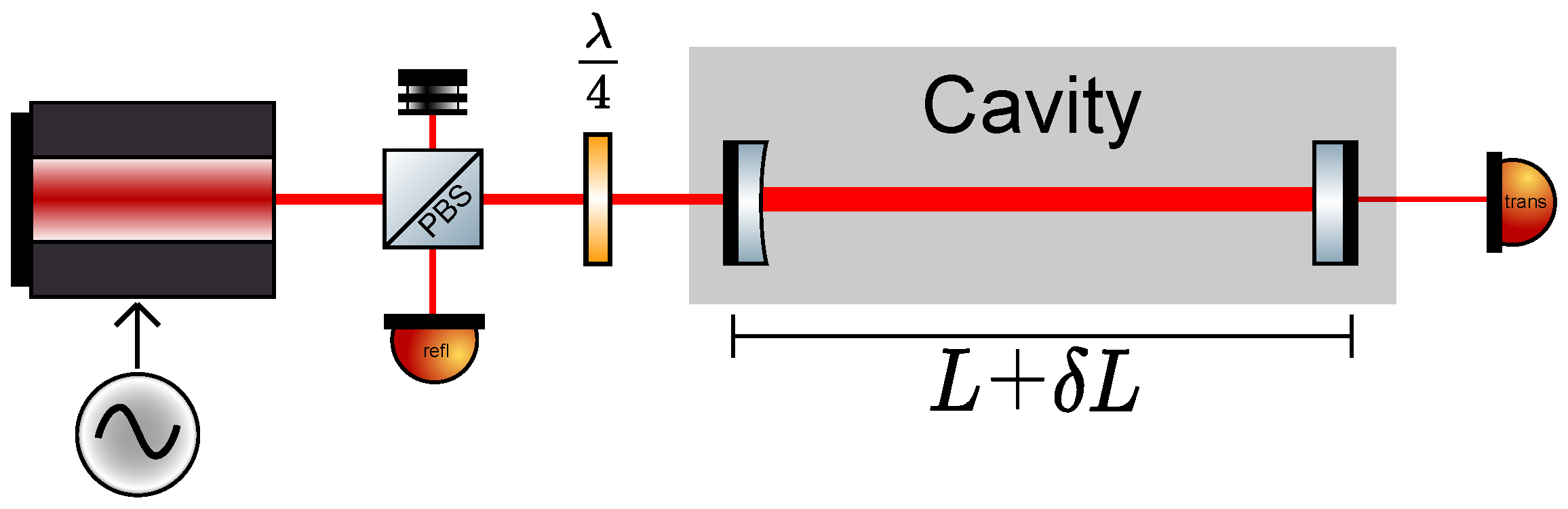
Here, we analysed the CRLB of an optical resonator that was probed with a strong frequency modulation, and thereby retaining multi-fringe operation, to determine if such a scheme can improve upon the limits of the two-beam topology analysed previously.

The interferometer topology we analysed is shown in Figure 7. We assumed an impedance-matched, loss-less resonator with a length L.

The static response of the reflected and transmitted optical power is given as:

$$\begin{array}{cc}\hfill P_{\mathrm{refl}}& \hfill =P_{\mathrm{in}}\left(1-\kappa \frac{{(1-R)}^2}{{(1-R)}^2+4R{sin}^2\left(\phi \right)}\right)=P_{\mathrm{in}}\left(1-\kappa \frac{1}{1+F{sin}^2\left(\phi \right)}\right)\hfill \end{array}$$

(27)

$$\begin{array}{cc}\hfill P_{\mathrm{trans}}& \hfill =P_{\mathrm{in}}\kappa \left(\frac{{(1-R)}^2}{{(1-R)}^2+4R{sin}^2\left(\phi \right)}\right)=P_{\mathrm{in}}\kappa \left(\frac{1}{1+F{sin}^2\left(\phi \right)}\right)\hfill \end{array}$$

(28)

with $F=4R/{(1-R)}^2$ as the Finesse coefficient. Here, we assumed that the cavity is in a steady-state, meaning that the laser frequency of all round-trips is the same. We assumed that the phase is simply given as $\phi ={\omega }_{0}L/c={\omega }_0/\left(2\mathrm{FSR}\right)$, with FSR as the free spectral range.

The Finesse of the resonator was approximated here [20] as:

$$\begin{array}{c}\hfill \mathcal{F}\approx \frac{\pi \sqrt{R}}{1-R}\end{array}$$

(29)

As is well known and calculated below, this cavity response provides a strong signal enhancement if a fixed operating point close to the resonance is chosen. In most applications of resonators, other readout methods are used, such as the Pound–Drever–Hall technique [21,22], but the underlying principle of signal enhancement near or at the resonance is the same. For direct, or DC, readout, the principle is similar to homodyne interferometers with a proportional relation between phase and power change that requires a simple calibration and offset subtraction.

To investigate if resonator readout can in principle be combined with multi-fringe operation, we modelled the cavity response to a (slowly) changing input frequency with a linear ramp (e.g., with $\omega ={\omega }_0+\Delta \omega t$) via:

$$\begin{array}{cc}\hfill P_{\mathrm{refl}}& \hfill =P_{\mathrm{in}}\left(1-\kappa \frac{1}{1+F{sin}^2(\phi +\Delta \mathsf{\Omega }·t)}\right)\hfill \end{array}$$

(30)

$$\begin{array}{cc}\hfill P_{\mathrm{trans}}& \hfill =P_{\mathrm{in}}\kappa \left(\frac{1}{1+F{sin}^2(\phi +\Delta \mathsf{\Omega }·t)}\right)\hfill \end{array}$$

(31)

$$\begin{array}{cc}\hfill & \hfill \mathrm{with}\Delta \mathsf{\Omega }=\frac{\Delta \omega }{2\mathrm{FSR}}\mathrm{and}\phi =\frac{{\omega }_0}{2\mathrm{FSR}}\hfill \end{array}$$

(32)

The linearised extraction of the phase from such a response could, for example, be realised by fitting an analytic model with a small number of free parameters. An infinite frequency ramp is of course unrealistic in practise, where one would use, for example, a triangular frequency modulation to provide cuts of effectively linear frequency change that extend over a fixed number of FSRs or one could also imagine using a sufficiently strong sinusoidal frequency modulation. In the case of the latter, the extraction of the phase would certainly require an even more complex phase extraction algorithm, but sinusoidal modulations can easily be realised, as demonstrated in DFM, and the number of free parameters is not excessive in comparison. For large frequency modulation depths, we can assume that the CRLB of a strong sinusoidal frequency modulation approximates the one for a linear frequency ramp, corresponding to our results for the two-beam interferometers (heterodyne and DFM) derived in Table 1. Hence, we used in the following the linear frequency ramp case to investigate the CRLB for this general class of frequency-shifted readout schemes to simplify the calculations, and we leave more detailed discussions about possible modulation schemes and readout algorithms for later studies.

The CRLB can again be calculated for a measurement period of $t\in [0,2\pi \frac{2\mathrm{FSR}}{\Delta \omega }]$ or respectively a frequency modulation of $\omega \in [{\omega }_0,{\omega }_0+4\pi \mathrm{FSR}]$, as outlined in [15].

Table 4. Cramer–Rao lower bound for the displacement power spectral density for the cavity response of different laser signals in a Fabry–Perot interferometer similar to Figure 7.

${\tilde{\mathit{L}}}^2$≥	Transmitted Output	Reflected Output
single frequency	$\frac{{(1+F{sin}^2\phi )}^3}{F^2{sin}^{2}2\phi }{\tilde{L}}_{\mathrm{s}}^2+\frac{{(1+F{sin}^2\phi )}^4}{4F^2{sin}^{2}2\phi }({\tilde{L}}_{\mathrm{e}+}^2+{\tilde{L}}_{\mathrm{d}}^2)$	$\frac{{(1+F{sin}^2\phi )}^3(1-\kappa +F{sin}^2\phi )}{\kappa F^2{sin}^{2}2\phi }{\tilde{L}}_{\mathrm{s}}^2+\frac{{(1+F{sin}^2\phi )}^4}{4F^2{sin}^{2}2\phi }({\tilde{L}}_{\mathrm{e}+}^2+{\tilde{L}}_{\mathrm{d}}^2)$
frequency ramp	$\frac{2{(1+F)}^{3/2}}{F^2}{\tilde{L}}_{\mathrm{s}}^2+\frac{{(1+F)}^{5/2}}{F^2(2+F)}({\tilde{L}}_{\mathrm{e}}^2+{\tilde{L}}_{\mathrm{d}}^2)$	$\frac{8{\kappa }^2}{-\frac{F^2{\kappa }^2}{{(F+1)}^{3/2}}-\frac{4(F+2)\kappa }{\sqrt{F+1}}-8\sqrt{(1-\kappa )(1-\kappa +F)}+8\sqrt{F+1}}{\tilde{L}}_{\mathrm{s}}^2+\frac{{(1+F)}^{5/2}}{F^2(2+F)}({\tilde{L}}_{\mathrm{e}}^2+{\tilde{L}}_{\mathrm{d}}^2)$

shows the CRLB of the cavity response for a single, constant frequency input and for a linearly shifting frequency input.

We found that the readout limits scaled in both cases with the Finesse coefficient and that in the case of a frequency ramp, the sensitivity was independent of the operating point, as desired. For a single frequency, the readout limit scaling with regards to the operating point was of course dependent on the Finesse coefficient (or the Finesse for that matter), with ${\tilde{L}}^2\propto 1/F$ close to the dark fringe (with $\phi \approx arcsin(1/\sqrt{F})$). In the case of the frequency ramp, the noise reduction scaling with the Finesse coefficient was generally weaker, but there was still a reduction, while a comparison with Table 2 reveals that the readout noise can be reduced below levels achievable in, for example, heterodyne interferometry. As discussed previously for single-frequency (DC) readout, other frequency-dependent electronic noise can be accounted for with ${\tilde{L}}_{\mathrm{e}+}$.

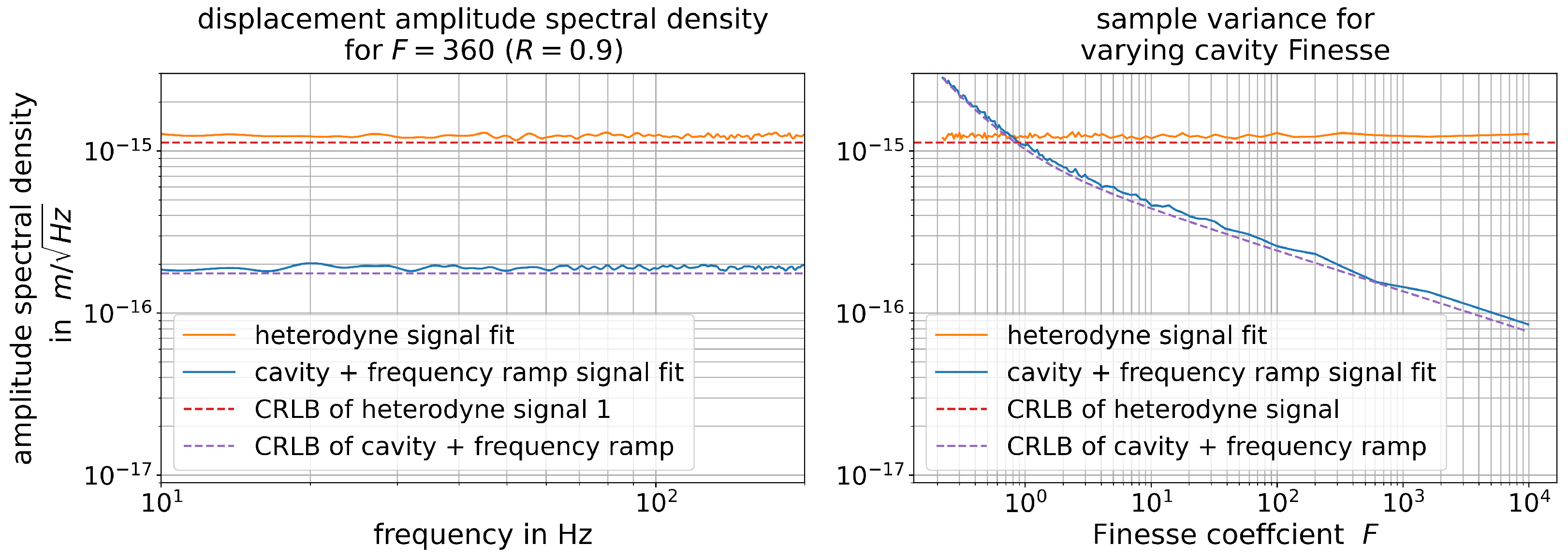
We verified this result with a numerical simulation, generating idealised signals for the readout of heterodyne interferometers and resonators probed in reflection by a frequency ramp. We then spoiled these signals with equal, simulated readout noise, either signal dependent, as required for shot-noise, or signal independent, as required for electronic or digitisation noise. We then extracted the phase from these time-series signals repeatedly by using a non-linear least-squares fit and analysed the noise level of the so-extracted phase. We show the simulated values and our derived dependencies of the CRLB in Figure 8 for different values of resonator Finesse in comparison with the value achieved for heterodyne interferometry and some example parameters. At Finesse levels above ⪆1, we found that the readout noise became lower than what can be achieved with non-enhanced multi-fringe readout techniques.

Intuitively, this result can be interpreted by realising that scanning over the response of a high Finesse resonator has a large range of tuning where basically no phase information is revealed, but readout noise is present, the plateau between resonances, and a small range near the resonances where strong phase information is available due to a large, condensed slope of the response. An increase in Finesse in a frequency-scanned resonator readout effectively reduces the time spent at the resonances, but the so-reduced averaging of noise is more than compensated by the improved signal-to-noise ratio at the resonances (assuming an optimal readout algorithm is applied). We found that this effect is true both for purely additive, constant readout noise sources, as well as for shot-noise, which scales with the detected optical power.

Before realising compact, multi-fringe sensors based on this frequency-scanned resonator readout, one will have to explore some crucial caveats. The resonator response we used here assumes a constant input frequency and does not account for finite cavity build-up time that deforms the response when a frequency scan is applied. This will limit the achievable, maximum frequency modulation rate, and the corresponding limitations of the resonant enhancement depend on the Finesse, the length of the resonator L, and the desired readout rate $f_{\mathrm{R}}$. Similarly, a higher Finesse and scanning rate will also require a larger bandwidth for signal detection and digitisation, providing another technical limitation to realistic implementations. Finally, if real modulations are applied, such as sinusoidal frequency modulations, the phase extraction algorithms need to be able to extract all relevant information in an optimal way and in real time. Independent of these and further challenges, a scheme such as the herein-sketched resonantly enhanced deep-frequency modulation interferometry (ReDFMI) can open a new range of sensitivity for compact, multi-fringe sensors that might not only benefit displacement sensing, but can also provide improvements with regard to tilt sensing and absolute ranging.

6. Conclusions and Outlook

The primary result of this article, the calculated Cramer–Rao lower Bound presented in Table 2 and Table 4, allows one to calculate the achievable interferometer precision a priori for a given or individually measured set of Gaussian, shot-, and digitisation noise. The dependence of the readout limit on the phase $\phi$ is compared in Figure 9 for the different discussed interferometer types.

For single-output setups (only one photodiode is measured), the calculated CRLB largely restates what is already well understood about interferometer precision, i.e., for the homodyne setup, we see that the shot-noise will either be optimal, or worst depending on whether the “bright” or the “dark” port of the interferometer is measured and its lower limit is dependant on the operating point of $\phi$. What initially may seem surprising is that the purely Gaussian noise readout limit diverges for both the “bright” and the “dark” port, while the shot-noise limit does not. The reason is that the total readout limit actually diverges in both cases (at exactly both fringes, a change of $\phi +ϵ$ and $\phi -ϵ$ cannot be differentiated due to the symmetry of the measured signal at that point). However, when considering only the shot-noise limit, the shot-noise converges faster to zero than the Fisher information in the vanishing signal.

The CRLBs for the heterodyne and quadrature setups showed no dependency on the operating point, as expected by their design. We also saw that for specific operating points, a homodyne (or to a small degree, a DFM interferometer) can potentially outperform these interferometers.

The DFM interferometer reveals itself to act as a hybrid between homodyne and heterodyne/quadrature interferometers. For a small modulation depth ($m\approx 0$, $J_0\left(2m\right)\to 1$), it of course acts as a homodyne interferometer with modulated readout [23], and for a large modulation depth ($m\gg 1$, $J_0\left(2m\right)\to 0$), it becomes even less dependant on the phase and performs as a heterodyne interferometer (which would be the usual operation mode for a DFM interferometer). Even though techniques such as DFMI have complex interferometer responses, their principle readout noise limitations are mostly similar to classic techniques such as heterodyne interferometers if the phase estimation is optimal. However, some residual, non-stationary readout noise behaviour is expected, when the operating point is changing, meaning if larger phase dynamics are recorded.

When measuring all outgoing ports from different interferometer setups, we found, e.g., that the total shot-noise limit was constant and identical for all setups ($1{\tilde{L}}_S^2$), as we would expect because the shot-noise only scales with the optical power, which was identical for all setups discussed here. Some homodyne setups measure however only one of their two output ports (e.g., the dark port for shot-noise-limited setups). We saw that if there is a phasemeter that can combine both output ports and reach the CRLB, there is no intrinsic need to operate at the dark fringe. However, operating at the dark fringe often provides other, technical benefits, such as the reduction of the detected power levels, readout complexity, and compatibility with recycling techniques [24].

As sensors based on DFM or other techniques can in principle achieve $1\mathrm{fm}/\sqrt{\mathrm{Hz}}$ level displacement sensitivities with available technologies, this provides a strong motivation to continue studying the necessary means of reducing the influence of other technical noise sources, with the goal of realising sensors that operate at, or close to, their CRLB.

Additionally, our analysis of the CRLB for Fabry–Perot resonators probed by strong laser frequency-scanning showed that there is a pathway to develop compact, multi-fringe-capable sensors with even lower sensitivities for future experiments and applications. While realising such enhanced sensor concepts will require overcoming a number of experimental challenges, it provides an exciting possibility to bridge the sensitivity gap between multi-fringe and sub-fringe readout techniques, opening up a new regime of achievable noise levels also for applications with multi-fringe motion.