Data-Driven Analysis of Cycling Behavior and Determinants of Bicycle Use Based on a Field Survey in Tehran, Iran

Abstract

Promoting cycling is an essential component of sustainable urban transportation, particularly in developing countries where bicycle use remains limited. This study proposes a two-step machine-learning framework to identify the predictors associated with bicycle use and cycling popularity in Tehran, Iran. A questionnaire survey was conducted among 1027 respondents, of whom 971 valid responses were retained for analysis. In the first step, the entire sample, including cyclists and non-cyclists, was analyzed using Decision Tree (DT), Random Forest (RF), and Artificial Neural Network (ANN) models to predict bicycle use. In the second step, the analysis focused exclusively on existing cyclists. A Cycling Popularity Index (CPI) was developed and classified into three levels, and ten machine-learning algorithms were evaluated. To address class imbalance, the Synthetic Minority Over-sampling Technique (SMOTE) was incorporated into model development. The results showed that Random Forest achieved the highest predictive performance in the first step, with bicycle-sharing availability, access to private cars, traffic congestion, occupation, proximity to public transportation, and social norms identified as the strongest predictors of bicycle use. In the second step, KNN-SMOTE achieved the best overall predictive performance, while Permutation Feature Importance identified occupation, age, social norms, perceived cycling safety, and physical condition as the most influential predictors of cycling popularity. The proposed framework demonstrates the value of combining multiple machine-learning algorithms with class-balancing techniques for analyzing imbalanced transportation datasets and provides a transferable methodology for similar studies in developing cities.

1. Introduction

Increasing urbanization exposes more people to traffic-related air pollution and its detrimental, expensive health effects [1,2]. Consequently, urban haze has increased over the past few decades along with the number of large cities [3]. Many cities are facing traffic congestion, which is one of the most obvious, prevalent, and immediate transportation challenges [4]. Congestion can be attributed to many factors, including rapid population growth, increased urbanization, inadequate transportation infrastructure, poor public transportation systems, and an increasingly large number of private cars [5]. As a result of traffic congestion, air pollution is significantly exacerbated [6,7,8,9].

The use of green modes of transportation can reduce air pollution, whereas traffic congestion tends to worsen it through longer commute times [10,11]. The bicycle is a sustainable and low-carbon mode of transportation [12,13,14]. Shared bikes can reduce short car trips and emissions from the transportation sector by up to 18% [15]. In heavily congested corridors, bike lanes could reduce congestion, but they have relatively limited impacts on energy consumption and emissions [15]. The analysis shows that using bicycles as a transport mode can significantly contribute to the UN Sustainable Development Goals (SDGs). Reduced toxic gas emissions and fewer traffic crashes contribute to SDG 3 (Good Health and Well-Being). SDG 8 (Decent Work and Economic Growth) can be improved by reducing transportation footprints. Improving air quality, reducing traffic congestion, and improving accessibility will help achieve SDG 11 (Sustainable Cities and Communities). Improving source efficiency and reducing transportation footprints will help achieve SDG 12 (Responsible Consumption and Production). Reducing greenhouse gas emissions will contribute to SDG 13 (Climate Action) [16,17].

Cycling is constrained by several factors such as weather dependency, requiring physical exertion, having a restricted speed, and inferior convenience in comparison to motorized options. On the other hand, personal vehicles typically offer greater comfort, flexibility, and accessibility. Promoting cycling as a daily travel option necessitates the identification of effective strategies. Various studies have examined methods for encouraging cycling and enhancing its appeal as an eco-friendly mode of transportation. This section reviews the existing literature to determine the primary influences and methods that support bicycle use.

It has been shown that cycling infrastructure influences users’ decisions to use shared bikes [18]. According to a case study in Sydney, cycling infrastructure should be integrated with job accessibility to promote cycling as a mode of transportation [19]. A study in Montreal, Canada, highlighted the importance of providing well-connected facilities across boroughs to address underperforming neighborhoods [20]. A bicycle can be used as a feeder mode on bicycle-metro trips. Cycling behavior is believed to be significantly influenced by the built environment. The behavior of transfer cycling around metro stations is often overlooked in transportation research [21]. Cycling is hindered by weather conditions, bicycle ownership, lack of paths or connections, and driver behavior; however, improving intersections, adding infrastructure, planting trees for shade, and providing affordable bicycles can motivate cycling [22]. The integration of the shared bike system into other forms of transportation, particularly at public transportation stops, and improving bicycle routes received the highest ratings [23]. A logit model was used to examine the relationship between 17 determinants of cycling mode. Among them were distance, population density, cycle paths, cycle lanes, traffic density, hilliness, temperature, sun, rain, wind, wealth, social status, children, green votes, bicycle performance, traffic risk, and parking costs [24,25]. Previous studies have applied data-driven approaches using shared bicycle trajectory data to objectively evaluate cycling environments and identify problematic road sections. Previous studies have applied both machine learning and multi-criteria decision-making approaches to evaluate cycling conditions. For example, Bayesian Networks and K-Nearest Neighbors (KNN) have been used for predictive modelling, whereas the Technique for Order Preference by Similarity to an Ideal Solution (TOPSIS) has been employed to evaluate cycling infrastructure, including parking facilities, intersection conditions, and bicycle lane occupancy, to support urban traffic management and planning [26]. Bikeshare demand is negatively affected by several factors, such as trip distance, temperature, precipitation, and air quality. Additionally, e-bikes can withstand distances, high temperatures, poor air quality, and precipitation [27].

The use of a hybrid discrete choice model showed how safety concerns restrict people from using bike lanes at street level when developing programs to promote cycling [28]. New immigrants to Toronto, Canada, reported fear of cycling as a result of their recent arrivals. Cycling fears came in a variety of forms; they were social, temporal, spatial, and dynamic. The two most common fears described by participants were fear of injury and fear of personal safety [29]. There is a greater concern for safety among female cyclists than male cyclists, based on the results from the study. Despite this, collision or injury fear did not differ by gender. Women expressed concerns about drivers’ verbal abuse and bullying, and how drivers treated cyclists [30]. In terms of cycling safety level, the “second road effects” refer to roads intersecting with roads where the crash occurred [31]. The crash injury outcomes of male and female cyclists differ significantly, with male cyclists suffering more severe injuries. Based on out-of-sample predictions, applying female parameters to cyclists could reduce severe injuries by 10.6% [32]. To promote cycling as an inclusive and accessible transportation option, it is crucial to understand sociodemographic differences and to ensure that tailored infrastructure is available to meet the needs of different groups [33]. Gender differences are more evident in cycling in comparison to other transport modes. Therefore, different studies have dealt with this issue. For women, cycling requires a higher level of utility than for men, and in higher utility environments, differences between men and women are almost nonexistent [24]. In spite of high-utility environments, older commuters still bike fewer miles than their younger counterparts. Children’s cycling behavior is influenced by their parents’ cycling behavior [34]. E-bikeshare choices are dominated by user heterogeneity in a multinomial logit model [27]. Bicycle training in schools can also play a crucial role in encouraging students to use bicycles more frequently. One-quarter of all children who had never cycled before training reported cycling more afterward [35]. The analysis found that trip distance, travelers’ income, number of cars or bicycles owned, and trip density significantly affect travelers’ travel mode decisions [36].

Table 1. Summary of reviewed papers.

Category	Subcategory	Authors/Citation	Main Findings
Influencing factors	Infrastructure and built-environment factors	Wu et al. (2024) [19]; Boisjoly et al. (2020) [20]; Shaaban (2020) [22]; Podgórniak-Krzykacz and Trippner-Hrabi (2021) [23]	Connectivity, bicycle infrastructure, network directness, built-environment characteristics, and integration with other transport modes are associated with cycling behavior and bicycle use.
Influencing factors	Cyclist-related and socio-demographic factors	Grudgings et al. (2021) [24]; Campbell et al. (2016) [27]; Bishop et al. (2024) [34]; Loo et al. (2020) [35]; Kashifi et al. (2022) [36]	Gender, age, training, family behavior, user heterogeneity, and trip characteristics are associated with cycling demand, mode choice, and cycling behavior.
Associated perceptions and outcomes	Safety perceptions and barriers	Márquez and Soto (2021) [28]; Ravensbergen et al. (2020) [29]; Graystone et al. (2022) [30]	Perceived crash risk, fear of cycling, bicycle-theft concerns, personal-security concerns, and interactions with motorized traffic may act as barriers to cycling.
Associated perceptions and outcomes	Objective safety outcomes	Ye et al. (2024) [31]; Barbour and Abdel-Aty (2024) [32]	Road-environment characteristics, cyclist characteristics, and gender are associated with perceived/objective cycling safety, crash risk, and injury-severity outcomes.

presents a summary of reviewed papers. In this table, papers are divided into three categories based on their subjects, including the role of infrastructure and built environment, safety, and cyclists’ characteristics.

This paper, in addition to its predecessors, seeks to determine the factors linked to bicycle usage, such as socio-demographic traits, environmental conditions, infrastructural elements, and social features, utilizing machine-learning methodologies. A two-step predictive method is proposed for achieving this target. The first step involves developing machine-learning models to differentiate between bicycle users and others. In the second phase, the examination concentrates solely on current cyclists to estimate varying cycling preferences. Moreover, various machine learning algorithms are analyzed systematically to identify the most reliable predictive models for each step.

The main contributions of this study are threefold. Initially, a new two-step machine-learning proposal is made, focusing on investigating bicycle adoption and cycling popularity as distinct elements. Second, it creates a Cycling Popularity Index (CPI) to depict varying degrees of cycling popularity among current cyclists. Third, it provides a comprehensive comparison of machine-learning algorithms, including three algorithms in the first step and ten algorithms in the second step, together with the application of SMOTE for handling class imbalance and Permutation Feature Importance (PFI) for model interpretation.

Accordingly, the objectives of this research are as follows:

• To identify the predictors associated with bicycle use among the general population using Decision Tree (DT), Random Forest (RF), and Artificial Neural Network (ANN) models.
• To develop and predict different levels of the Cycling Popularity Index (CPI) among existing cyclists through a comprehensive comparison of ten machine-learning algorithms.
• To compare the predictive performance of the evaluated machine-learning models and identify the most suitable model for each analytical step.
• To interpret the contribution of the identified predictors using feature importance analysis and provide evidence that can support cycling-related transportation planning.

2. Materials and Methods

This study is set to forecast bicycle journeys and the trend in bicycle usage via the application of Machine Learning (ML) techniques. This purpose involves two steps that are evaluated.

2.1. Step 1-Method

The initial objective was to identify the factors related to bicycle usage within the general population. Consequently, the target variable was defined as bicycle usage for daily trips (bicycle user vs. non-user), categorizing it as a binary classification problem. The predictor variables utilized in this step, identical to those used in the second step, are outlined in

Table 2. Input features for ML modeling.

Variable	Abbreviation
Gender	GEN
Age (years)	AGE
Physical status	PHY
Education	EDU
Monthly income (USD)	INC
Frequency of daily trip	NDT
Average weight of accompanied luggage in daily trips	CLD
Frequency of days with access to a private car in a week	APC
Walking distance to the first public transit station (minutes)	DNS
What is your opinion about cycling safety on the path to your destinations?	RSC
Job	JOB
Is there any bike-sharing facility in your living district?	ESB
How much are social norms important for you to use a bicycle for daily trips?	ESN
What is the average longitudinal grade on your path to work/school/shopping or other purposes?	SSC
What is the air pollution status in your living district?	AIP
What is the traffic condition in your living district?	TRC
What is the probability of finding proper parking at your destination?	FCP
What is the probability of finding suitable bike parking at your destination?	FBP

. Explanatory variables such as socio-demographic factors, travel-related aspects, infrastructural elements, and perceptual characteristics were chosen after a thorough examination of the relevant scholarly literature.

To develop the prediction models, three representative machine-learning algorithms were selected: Decision Tree (DT), Random Forest (RF), and Artificial Neural Network (ANN). These models represent different learning approaches, with DT providing an interpretable tree-based structure, RF representing an ensemble learning approach with strong predictive capability, and ANN capturing complex nonlinear relationships among variables. Since the objective of this step was not only prediction but also identification of important predictors associated with bicycle use, these models provided a balance between predictive performance and interpretability.

Models based on the three preceding approaches (DT, RF, and ANN) were created in Python (Version 3.14.6) utilizing the scikit-learn library. Scikit-learn delivers a wide array of supervised and unsupervised machine learning methods, prioritizing computational speed, user-friendly execution, and thorough documentation.

Before developing the model, nominal categorical variables were initially encoded with One-Hot Encoding to prevent the imposition of artificial ordinal relationships between the categories. Continuous variables were normalized using the MinMaxScaler, particularly to improve the performance of the ANN. The presence of missing values was rare, and these were filled in with the median value from respondents sharing similar socio-demographic profiles (such as age, occupation, and educational background).

Finally, the dataset was partitioned into training (70%), validation (15%), and test (15%) segments. A systematic trial-and-error procedure was used to optimize hyperparameters with only the training and validation datasets. Various hyperparameter settings were assessed for each algorithm, and the setup producing the maximal validation accuracy was picked. The hyperparameters selected for both the first and second step of the machine learning models, as finalized, are listed in

Table 3. Hyperparameters used for each machine learning method based on the scikit-learn library.

ML Method	Hyperparameter	Value
DT	Criterion	Entropy
	Max_depth	3
RF	N_estimators	30
	Criterion	Entropy
	Max_depth	4
ANN	Hidden_layer_sizes	5
	Max_iter	110
	Solver	SGD
	Learning_rate_init	0.1
	Activation	ReLU

.

Following the selection of optimal hyperparameters, they were uniformly applied in all subsequent analyses. Stratified five-fold cross-validation was then used to evaluate the predictive performance of the final models. By isolating hyperparameter optimization from the ultimate model evaluation, the chance of over-optimistic performance assessments was diminished.

2.2. Step 2-Method

For the second phase, the analysis was confined exclusively to existing cyclists to ascertain the factors influencing different bicycle use levels. The Cycling Popularity Index (CPI), serving as the target variable for the classification models, was developed. The explanatory variables were identical to those used in the first-step analysis (Table 2), allowing the same set of predictors to be evaluated for their ability to explain variations in cycling popularity rather than bicycle usage itself.

Three variables were used to construct the CPI: average daily cycling duration, the number of time-of-day intervals in which cycling occurred, and the number of seasons during which respondents used a bicycle.

Individuals were allowed to choose multiple time periods and seasons. Thus, the number of selected time intervals varied from 1 to 9, whereas the number of selected seasons ranged from 1 to 4. The variables were classified as count variables due to their values representing the actual number of selected intervals and seasons.

Unlike the other two components, average daily cycling duration cannot be considered a count variable since it measures a continuous time span. For constructing the index, the lowest daily cycling duration was taken to be 15 min (0.25 h), whereas the maximum was fixed at 3 h per day. Consequently, responses signaling more than two hours of daily cycling were given a value of three hours, which corresponds to the highest value employed in the index.

To ensure that variables with larger ranges do not overly influence the index, each component was normalized to a 0 to 1 scale. The normalized daily cycling-duration component was calculated as Equation (1):

$${\mathrm{D}}_{\mathrm{i}}^{*}={\displaystyle \frac{{\mathrm{D}}_{\mathrm{i}}-{\mathrm{D}}_{\min }}{{\mathrm{D}}_{\max }-{\mathrm{D}}_{\min }}}$$

(1)

where: D_i: the assigned hourly value for respondent (i); D_min: minimum duration of cycling; and D_max: maximum duration of cycling.

The normalized number of time-of-day intervals was calculated as Equation (2):

$${\mathrm{T}}_{\mathrm{i}}={\displaystyle \frac{{\mathrm{T}}_{\mathrm{i}}-1}{9-1}}$$

(2)

where: T_i: The number of selected time-of-day intervals.

The normalized seasonal-use component was calculated as Equation (3):

$${\mathrm{S}}_{\mathrm{i}}={\displaystyle \frac{{\mathrm{S}}_{\mathrm{i}}-1}{4-1}}$$

(3)

where: S_i: The number of seasons during which the respondent reported cycling.

The Cycling Popularity Index (CPI_i) was calculated using a multiplicative formulation in which the three components were combined without applying differential weighting coefficients, as shown in Equation (4):

$$\mathrm{C}\mathrm{P}{\mathrm{I}}_{\mathrm{i}}={\mathrm{D}}_{\mathrm{i}}^{*}\times {\mathrm{T}}_{\mathrm{i}}\times {\mathrm{S}}_{\mathrm{i}}$$

(4)

In theory, the index has a range of 0 to 1. Longer daily riding times, riding at more different times of the day, and riding a bicycle in more seasons are all indicated by higher values. Since there was no solid theoretical or empirical evidence to suggest that one component should be more important than the others, equal weights were given.

The 33rd and 67th percentiles of the continuous index’s observed distribution were used to create three categories for the supervised classification analysis. Respondents were categorized as having low cycling-use intensity if their index values were at or below the 33rd percentile. Respondents over the 67th percentile were categorized as having high cycling-use intensity, while those with values between the 33rd and 67th percentiles were classed as having moderate cycling-use intensity.

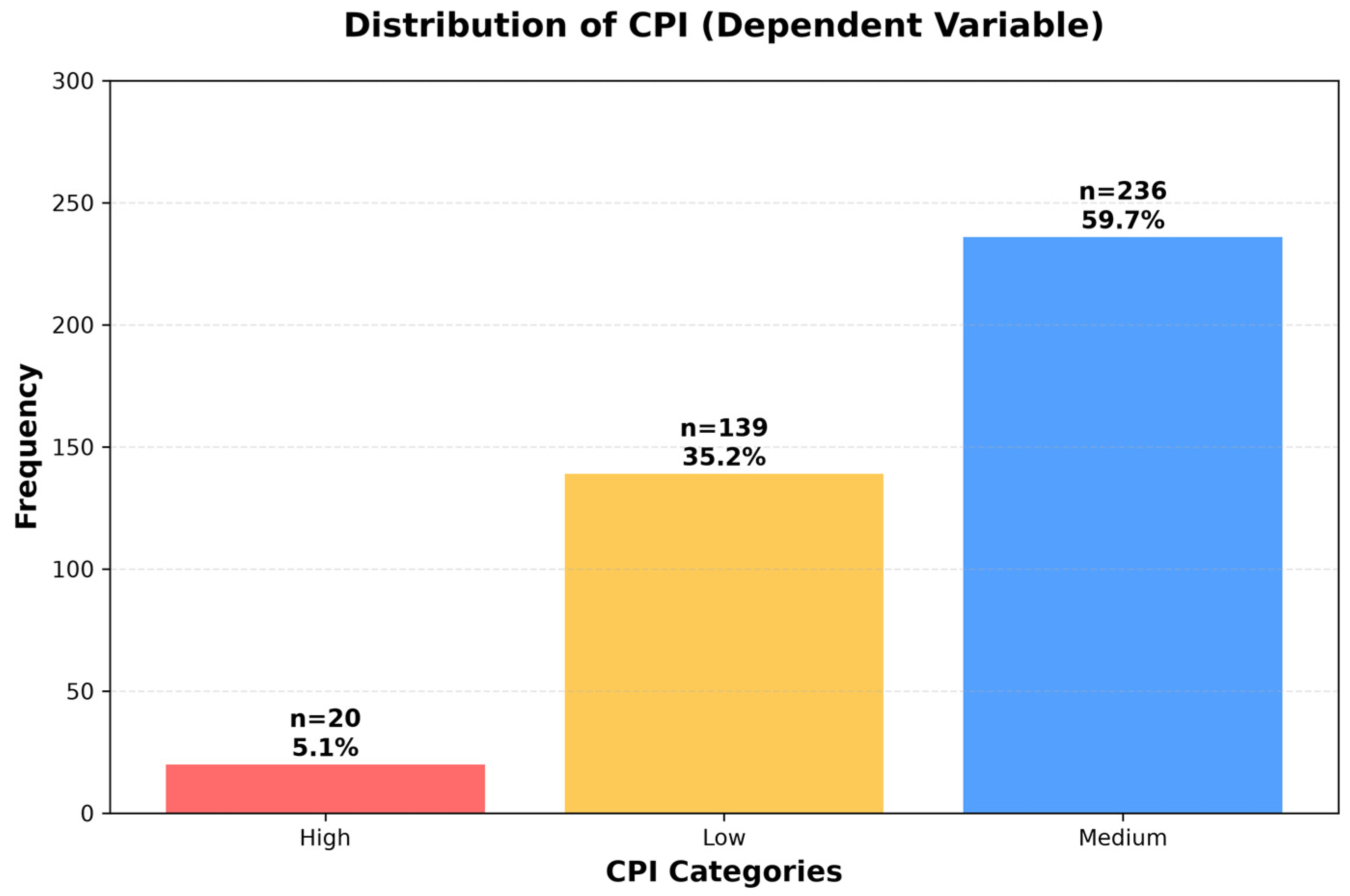
The normalized CPI ranges from 0 to 1 and was classified into three levels: Low (0.00–0.33), Medium (0.34–0.67), and High (>0.67). The detailed frequency and relative-frequency distributions of the three CPI components daily cycling duration, number of time-of-day intervals, and number of cycling seasons are provided in Appendix C.

Table 4. Bicycle popularity variable.

Variable	Code	Categories/Range
Average duration of cycling in a given day (hours)	-	0.25 to more than 3
The frequency of times when bicycles are used (time of a day)	Multiple choices	6:00–7:59
		8:00–9:59
		10:00–11:59
		12:00–13:59
		14:00–15:59
		16:00–17:59
		18:00–19:59
		20:00–21:59
		22:00–23:59
The frequency of seasons when bicycles are used in a given year	Multiple choices	Spring
		Summer
		Fall
		Winter

reports the number of responses in each category as well as the precise cut-off values.

Ten supervised machine-learning algorithms representing various learning methods were assessed to determine the best predictive model for bicycle utilization and the CPI. DT, RF, ANN, Logistic Regression (LR), Support Vector Machine (SVM), K-Nearest Neighbors (KNN), Gradient Boosting (GB), AdaBoost, Gaussian Naïve Bayes (GNB), and a Voting Ensemble classifier are some of these. A thorough comparison of several classification techniques is made possible by the chosen algorithms, which include tree-based, linear, probabilistic, instance-based, kernel-based, neural-network, and ensemble-learning approaches.

To classify observations, tree-based algorithms (DT and RF) divide the feature space recursively. While RF increases prediction accuracy and robustness by combining many randomized decision trees, DT offers a clear and understandable decision structure.

An ANN is a nonlinear learning model made up of interconnected processing units that can learn intricate correlations between variables. Because of its adaptability, it can capture nonlinear interactions that are commonly found in research on travel behavior [37].

LR is a statistical classification model that functions as an interpretable baseline classifier and uses a logistic function to estimate class probabilities [38].

SVM can efficiently model nonlinear decision boundaries through kernel functions and finds an ideal separation hyperplane by maximizing the margin between classes [39].

KNN is a non-parametric instance-based learner that categorizes observations based on the majority class of their closest neighbors in the feature space [40].

In order to enhance prediction performance, weak learners are successively combined using boosting-based ensemble techniques such as GB and AdaBoost [41]. Based on Bayes’ theorem and assuming conditional independence between predictors, GNB is a probabilistic classifier [42]. Lastly, to increase prediction stability, the Voting Ensemble uses majority voting to combine the predictions of several classifiers [43].

There was a significant class imbalance in the CPI dataset, with very few observations falling into the group of high cycling popularity. Machine-learning algorithms may be biased toward the majority classes and less able to identify minority observations as a result of this imbalance.

The training dataset was subjected to the Synthetic Minority Over-sampling Technique (SMOTE) in order to mitigate this issue. By interpolating across nearby samples, SMOTE creates artificial minority-class observations, improving class balance without repeating preexisting data [44]. The original and SMOTE-balanced datasets were used to train each classifier, and their results were then compared (The SMOTE settings is available in Appendix D).

Several complementary performance metrics were used to assess each classifier’s predicted performance. Accuracy was used to measure overall classification performance, whereas F1-score, Precision, and Recall were used to gauge the accuracy of class-specific predictions. The Weighted F1-score was chosen as the main performance metric because it takes into consideration both the imbalance in the CPI classification problem and the trade-off between precision and recall. Additionally, each model’s accuracy in identifying the minority category was assessed by explicitly looking at the F1-score of the High class.

The evaluation metrics are defined as follows.

2.3. Models’ Assessment

Different models based on the three mentioned methods are evaluated through these indices:

• Accuracy

The percentage of accurate forecasts, both true positives and true negatives, among all predictions is known as accuracy. It gives a broad idea of the model’s overall performance [45]. Equation (5) is used to calculate the accuracy index.

$$\mathrm{A}\mathrm{c}\mathrm{c}\mathrm{u}\mathrm{r}\mathrm{a}\mathrm{c}\mathrm{y}={\displaystyle \frac{\mathrm{T}\mathrm{P}+\mathrm{T}\mathrm{N}}{\mathrm{T}\mathrm{P}+\mathrm{T}\mathrm{N}+\mathrm{F}\mathrm{P}+\mathrm{F}\mathrm{N}}}$$

(5)

where: TP = True Positives (correctly predicted positive cases); TN = True Negatives (correctly predicted negative cases); FP = False Positives (incorrectly predicted positive cases); and FN = False Negatives (incorrectly predicted negative cases).

• Precision

The percentage of correctly predicted positive cases among all cases the model predicts as positive is known as precision. It shows how trustworthy positive predictions are [45]. Equation (6) is used to calculate the precision index.

$$\mathrm{P}\mathrm{r}\mathrm{e}\mathrm{c}\mathrm{i}\mathrm{s}\mathrm{i}\mathrm{o}\mathrm{n}={\displaystyle \frac{\mathrm{T}\mathrm{P}}{\mathrm{T}\mathrm{P}+\mathrm{F}\mathrm{P}}}$$

(6)

• Recall

The percentage of real positive cases that the model properly identified is known as recall. It demonstrates how well all positive cases are captured by the model [45]. Equation (7) is used to calculate the recall index.

$$\mathrm{R}\mathrm{e}\mathrm{c}\mathrm{a}\mathrm{l}\mathrm{l}={\displaystyle \frac{\mathrm{T}\mathrm{P}}{\mathrm{T}\mathrm{P}+\mathrm{F}\mathrm{N}}}$$

(7)

• F1 Score

A balanced indicator of classification ability, especially for datasets with unbalanced class distributions, is the F1-score, which is the harmonic mean of precision and recall [45]. Equation (8) is used to determine the F1-score.

$$\mathrm{F}1\mathrm{s}\mathrm{c}\mathrm{o}\mathrm{r}\mathrm{e}=2\times {\displaystyle \frac{\mathrm{P}\mathrm{r}\mathrm{e}\mathrm{c}\mathrm{i}\mathrm{s}\mathrm{i}\mathrm{o}\mathrm{n}\times \mathrm{R}\mathrm{e}\mathrm{c}\mathrm{a}\mathrm{l}\mathrm{l}}{\mathrm{P}\mathrm{r}\mathrm{e}\mathrm{c}\mathrm{i}\mathrm{s}\mathrm{i}\mathrm{o}\mathrm{n}+\mathrm{R}\mathrm{e}\mathrm{c}\mathrm{a}\mathrm{l}\mathrm{l}}}$$

(8)

Model selection was not predicated on a single statistic since several approaches were compared. Rather, the ability to identify the minority (High) class and total predictive accuracy were taken into account simultaneously. The final prediction model was chosen to be the classifier that best balanced these factors.

Permutation Feature Importance (PFI) was used to understand the chosen model. In contrast to impurity-based feature importance, PFI is model-agnostic and calculates each predictor’s contribution by calculating the decrease in prediction performance following a random permutation of the feature’s values. More influential variables are those that result in greater declines in prediction performance. As a result, PFI rather than the internal important metrics of specific algorithms served as the basis for the model’s final interpretation.

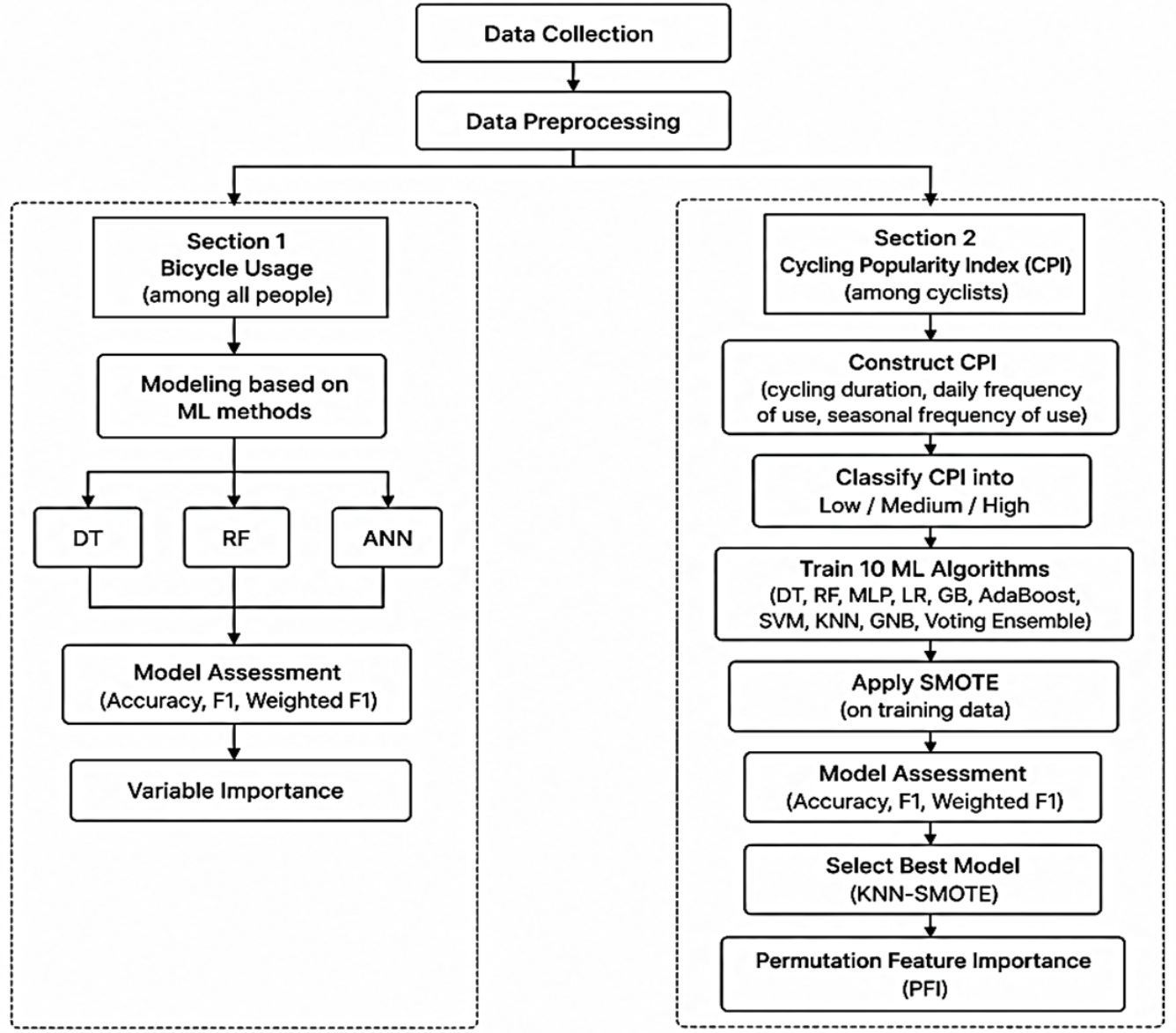
The research flowchart to follow the details of each step is given in Figure 1.

3. Data

A dataset and a suitable case study are necessary when using machine-learning techniques. Iran’s capital, Tehran, was chosen as the case study for this investigation. The investigation was carried out in two phases, as previously described. In order to estimate whether people use bicycles for everyday travel, the first step took into account the full sample, including both cyclists and non-cyclists. In order to examine the variables linked to varying degrees of bicycle popularity, the second step concentrated solely on current cyclists.

Two recruitment strategies were employed during the data collection period. An online survey was initially made using Google Forms and distributed via social media platforms like Telegram and WhatsApp in order to reach both cyclists and non-cyclists. During the first round of data collection, it was discovered that there were not enough respondents who regularly used bicycles for daily transportation for the second-step analysis. Thus, additional data was obtained by conducting in-person interviews with bikers observed in public spaces. Interviews with other road users, such as walkers, persons using public transportation, and those accessing parked cars, were conducted in this phase in order to include both bicycle users and non-users in the dataset.

The chosen recruitment approach cannot be regarded as a pure stratified random sampling procedure since a full sampling frame of Tehran inhabitants was not accessible and random selection of persons within each group was not practical. Rather, a stratified quota-based strategy was used, whereby the distribution of responders among predetermined groups was continuously tracked during the data collection process. Because prior research has shown that gender, age, and income categories are relevant to travel behavior, they were taken into consideration as sampling strata. In order to improve the final sample’s balance, more recruitment efforts were focused on groups with fewer replies whenever a particular group became overrepresented or underrepresented. This strategy lessens the likelihood that a specific recruiting strategy or demographic group would predominate in the final dataset, even if it cannot totally eradicate selection bias.

The questionnaire was developed based on important variables identified through the literature review. The collected variables included socio-demographic characteristics (gender, age, education level, monthly income, and occupation), travel-related characteristics (number of daily urban trips and carried load), accessibility variables (distance to the nearest metro/bus station), cycling-related perceptions (cycling safety and social norms), built-environment characteristics (availability of bicycle lanes, bicycle-sharing systems, bicycle parking, and car parking), and environmental conditions (hilliness, air pollution, and traffic congestion).

Data collection was conducted from August 2020 to March 2021 through both electronic questionnaires and field interviews. In total, 1027 responses were collected. During the data preprocessing stage, 56 observations were removed due to inconsistent responses, missing information, or incorrect answers to control questions. Consequently, 971 valid observations were retained for model development. For the second step of the analysis, 400 respondents who reported bicycle use were extracted from the complete dataset to develop the bicycle popularity model. Out of the initial 400 responses, 395 valid observations remained after data cleaning. Each observation represents one respondent, while each column represents one explanatory variable.

Sample size is an important consideration in predictive modeling because an adequate number of observations can contribute to more stable model estimation and more reliable assessment of model generalizability. However, a larger sample size does not, by itself, guarantee higher predictive accuracy, which also depends on factors such as data quality, class distribution, predictor informativeness, and model specification. For the present survey, the minimum sample size was estimated using Equation (9). Considering Tehran’s population of approximately 10 million, a 95% confidence level, and a 5% precision level, the estimated minimum survey sample size was 385 respondents. The final dataset included 971 valid observations, exceeding this survey-based requirement. For the second-step analysis, 395 bicycle users were available. Because the CPI classes within this subsample were imbalanced, model performance was evaluated using multiple classification metrics and the effect of class balancing was separately examined using SMOTE. Thus, the sample-size calculation is used here to support the adequacy of the overall survey sample rather than to imply that increasing the number of observations necessarily improves predictive accuracy.

Before model development, descriptive statistical analyses were conducted to examine the characteristics and distributions of all variables. A detailed summary of descriptive statistics for both steps is provided in Appendix A and Appendix B.

As the number of data points increases in machine-learning models, the accuracy will also increase. A sufficient sample size can be determined based on Equation (9).

$$\mathrm{n}\ge \mathrm{N}{\left[1+{\displaystyle \frac{\mathrm{N}-1}{\mathrm{p}\mathrm{q}}}{({\displaystyle \frac{\mathrm{d}}{{\mathrm{Z}}_{\frac{\mathsf{\alpha }}{2}}}})}^2\right]}^{-1}$$

(9)

where: n: Sample size, number of required samples. N: Population size, Tehran population (about 10 million). Z: 1.96 for 95% confidence level. p, q: The quality characteristics which are to be measured. Where no previous experience exists, the value of p is taken as 0.5 and q = 1 − p = 0.5. d: The desired level of precision is considered 5%.

According to Equation (9), there must be at least 385 participants in the experiment. As a result, the data collected is appropriate for both steps.

In order to reduce sampling bias, stratified quota-based sampling was used. To achieve this, it is necessary to ensure that different subgroups of the selected people are adequately represented. Due to the influence of age, gender, and income level on transportation preferences, the population was stratified by age, gender, and income.

Before developing the model, descriptive statistical studies were carried out to look at the features and distributions of each study variable.

4. Results

As previously stated, this study is divided into two sections: the first is modeling using all 971 appropriate data to promote bicycling among all individuals. In order to increase bicycle utilization among cyclists, 400 out of 971 riders were filtered for a secondary study. Out of the initial 400 responses, 395 valid observations remained after data cleaning.

4.1. Step 1-Results

The k-fold cross-validation method was used to generate the models in Section 1. This means that every modeling procedure uses all of the data for training and testing by splitting the dataset into k folds and training and testing on each fold in turn. In this study, k = 5 was chosen as the number of folds. The average values of these five folds will be used to compute the final indices, which include accuracy, precision, F1 score, and recall.

Table 5. Comparative evaluation summary in Section 1 in DT, RF, and ANN methods.

Model	Fold	Accuracy	Precision	Recall	F1 Score
DT	1	0.718	0.761	0.718	0.728
	2	0.722	0.734	0.722	0.725
	3	0.711	0.728	0.711	0.717
	4	0.686	0.685	0.686	0.684
	5	0.686	0.699	0.686	0.689
	Avg.	0.704	0.721	0.705	0.709
RF	1	0.785	0.808	0.785	0.791
	2	0.742	0.769	0.742	0.748
	3	0.799	0.819	0.799	0.803
	4	0.768	0.808	0.768	0.777
	5	0.784	0.822	0.784	0.791
	Avg.	0.775	0.805	0.776	0.782
ANN	1	0.728	0.729	0.728	0.728
	2	0.747	0.768	0.747	0.751
	3	0.753	0.763	0.753	0.756
	4	0.809	0.823	0.809	0.812
	5	0.732	0.731	0.732	0.731
	Avg.	0.754	0.763	0.754	0.756

displays the outcomes of the modeling in Section 1.

Table 5 illustrates that RF and ANN outperformed DT in all evaluation metrics. RF was chosen for additional interpretation because it performed the best overall out of the three models that were assessed.

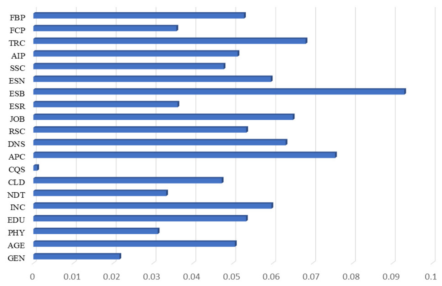
Figure 2 shows the relative relevance of the 19 input features, which was determined using the RF model. The scikit-learn implementation’s mean decrease in impurity measure was used for feature significance analysis. Instead of being averaged throughout the cross-validation folds, the significance values were taken from the final trained RF model. As a result, each predictor’s relative contribution to the final model’s predictive structure is represented by the reported values.

It should be mentioned that variables with more categories or more possible split points may be biased towards impurity-based feature significance assessments. As a result, rather than being indicative of causal impacts, the rankings are viewed as predictive relevance indicators. Additionally, this study did not assess feature importance consistency across various cross-validation folds; as a result, the ranking that is reported relates to the final RF model and could be impacted by sampling variability.

Based on the feature importance results shown in Figure 2, the following conclusions can be drawn.

The most effective feature is “existence of a bicycle-sharing system/ESB”. The second most important feature is “access to a personal car/APC”. The next three important features are “traffic congestion/TRC”, “job/JOB”, and “distance (In minutes) from the nearest metro/bus station/DNS”. The sixth most important feature is “social norms/ESN” and its effects on using or not using a bicycle.

4.2. Step 2-Results

The original imbalanced dataset was used to train ten classification algorithms: DT, RF, Multi-Layer Perceptron (MLP), LR, GB, AdaBoost, SVM, KNN, GNB, and a Voting Ensemble classifier. For every model, an 80% training and 20% testing split was employed. Three ordinal groups made up the dependent variable, the Cycling Popularity Index (CPI): Low (28 observations), Medium (47 observations), and High (4 observations). The High class only made up about 5% of the sample; hence, most baseline models had trouble identifying this tiny group.

The Synthetic SMOTE was limited to the training data in order to reduce class imbalance. To provide a fair comparison, all ten classifiers were then retrained using the balanced training set and assessed on the same unaltered test set. Overall, SMOTE enhanced the high-class recognition for many algorithms, although the degree of improvement varied significantly throughout models.

With an accuracy of 63.29%, a weighted F1-score of 63.79%, and an F1-score of 0.40 for the High class, KNN-SMOTE outperformed all other classifiers in terms of overall predictive performance balance. Although SVM-SMOTE had perfect precision (1.00) and an identical F1-score for the High category, its recall was just 0.25, meaning that the majority of High-class observations were missed. Minority-class prediction was similarly improved by AdaBoost-SMOTE and DT-SMOTE, with F1-High values of 0.286 and 0.308, respectively.

Three of the four High observations were accurately identified by Logistic Regression-SMOTE, which had the highest recall for the High class (0.75). However, a high number of false-positive predictions is indicated by its low precision (0.158), which lowered its weighted F1-score and total accuracy. RF-SMOTE, on the other hand, was unable to accurately classify any High-class observation while maintaining competitive overall accuracy (63.29%). Despite having respectable overall performance, Neural Network-SMOTE and Gradient Boosting-SMOTE also generated an F1-High of zero.

Table 6. Overall performance of SMOTE-balanced classification models.

Model	Accuracy	Weighted F1	F1 (High)	Precision (High)	Recall (High)
AdaBoost	0.557	0.568	0.308	0.222	0.500
Decision Tree	0.570	0.557	0.286	0.333	0.250
Gradient Boosting	0.532	0.500	0.000	0.000	0.000
KNN	0.633	0.638	0.400	0.333	0.500
Logistic Regression	0.468	0.498	0.261	0.158	0.750
Naïve Bayes	0.519	0.538	0.200	0.125	0.500
Neural Network	0.608	0.605	0.000	0.000	0.000
Random Forest	0.633	0.602	0.000	0.000	0.000
SVM	0.620	0.586	0.400	1.000	0.250
Voting Ensemble	0.582	0.595	0.286	0.200	0.500

Note: Bold values indicate the best performance for each metric.

’s findings demonstrate that choosing a model in a highly imbalanced classification situation requires more than just overall accuracy. The impact of SMOTE was highly algorithm-dependent: although some high-capacity or distribution-dependent models only slightly improved, KNN and SVM gained the most in terms of minority-class recognition. KNN-SMOTE was chosen as the final model based on overall accuracy, weighted F1-score, and the capacity to simultaneously identify the uncommon High CPI class.

Table 7. Classification report of the selected KNN-SMOTE model.

Class	Precision	Recall	F1-Score	Support
Low	0.567	0.607	0.586	28
Medium	0.721	0.660	0.689	47
High	0.333	0.500	0.400	4
Macro average	0.540	0.589	0.558	79
Weighted average	0.647	0.633	0.638	79

displays the comprehensive classification report for the chosen KNN-SMOTE model. The Medium class has the best model performance (F1 = 0.689), followed by the Low class (F1 = 0.586). The F1-score for the High class was 0.400, with precision of 0.333 and recall of 0.500. This outcome marked a significant improvement over the corresponding baseline model, which was unable to identify the minority class, even while the High class’s absolute performance remained moderate. KNN-SMOTE demonstrated the most balanced performance among the three CPI categories, as confirmed by the weighted F1-score of 0.638.

The classification report of Table 7 (with 28 Low, 47 Medium, and 4 High) is based only on the 79 test-set observations. These 79 observations are a representative subset of the 395 cyclists, and they reflect the original class distribution within the cyclist sub-population

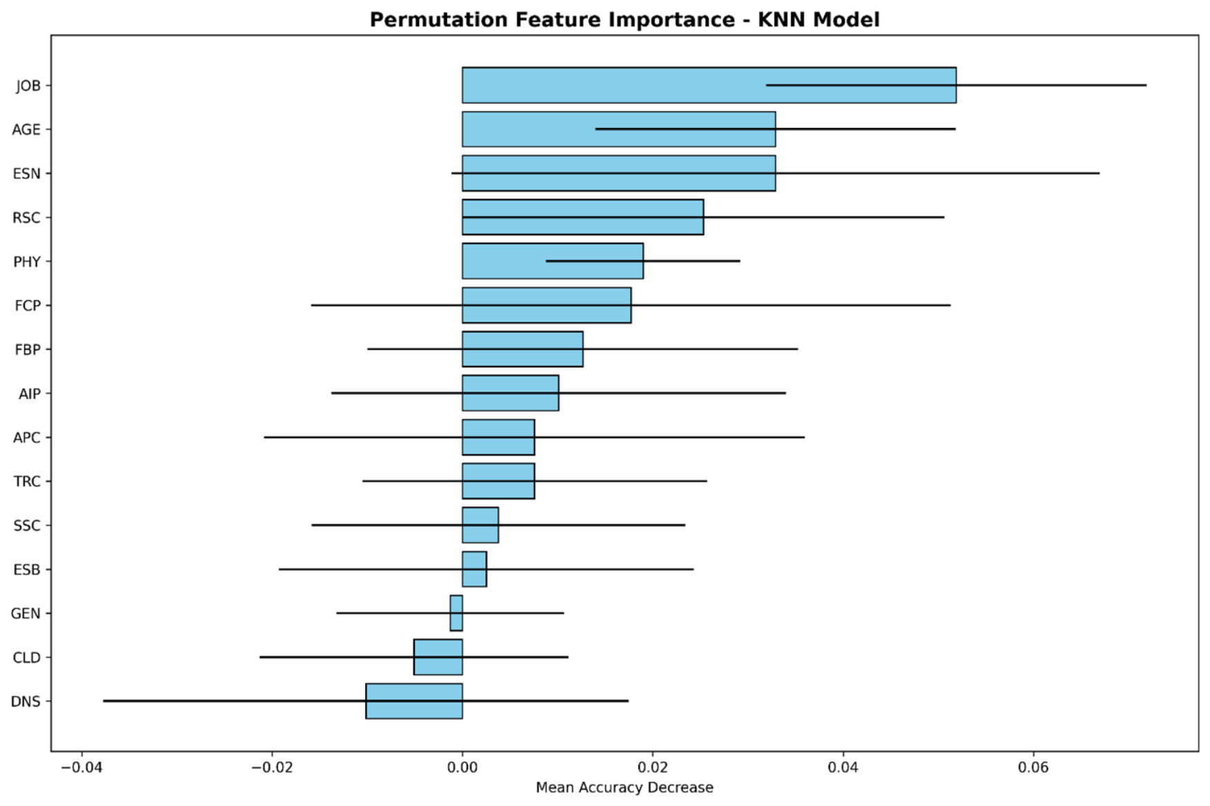
Permutation Feature Importance (PFI) was used to interpret the chosen KNN-SMOTE model. PFI is a model-agnostic technique that measures the decrease in predictive accuracy that results from randomly rearranging each predictor’s values. A greater decline suggests that the model depends more heavily on that characteristic. This method is appropriate for distance-based classifiers like KNN and offers a straightforward and computationally effective evaluation of variable importance [46,47,48]. Figure 3 presents the findings.

The most significant predictor was occupation (JOB), which caused the biggest mean drop in model accuracy (0.052) following permutation. With relevance ratings of roughly 0.033, age (AGE) and the significance of social norms (ESN) came next. These findings show that social judgments and sociodemographic traits both significantly influenced how popular cycling was classified. Physical condition (PHY) and perceived cycling safety (RSC) also had significant effects, with significance values of 0.019 and 0.025, respectively.

Air pollution (AIP), traffic conditions (TRC), parking availability (FCP and FBP), and daily automobile access (APC) all had lower significance values, typically falling between 0.008 and 0.018. Therefore, these parameters had less of an impact on the KNN-SMOTE model’s predictive structure than age, occupation, social norms, safety perceptions, and physical condition. However, some variables, especially ESN and FCP, have unusually significant standard deviations that suggest ambiguity in their estimated importance. This could be due to the small test-sample size and random variation across permutation repeats.

Overall, the PFI results show that elements connected to infrastructure and the environment had a very minor impact on KNN-SMOTE predictions, while sociodemographic and perceptual variables, particularly occupation, age, and social norms, were the main contributors. These results make the chosen model easier to understand, but they also imply that future research should look into potential interactions between the most important variables and confirm their stability using bigger sample sizes.

5. Discussion

This study investigated cycling patterns from two complementary perspectives using a two-step predictive modeling approach. In the first step (Bicycle Usage), the complete sample of respondents was analyzed to identify the primary factors associated with daily bicycle use. In the second step (Cycling Popularity Index), the analysis was restricted to current cyclists to examine the factors associated with different levels of cycling popularity as measured by the CPI. Comparison of several machine-learning algorithms showed that RF achieved the best predictive performance in the first step, whereas KNN combined with SMOTE provided the most balanced performance in the second step by improving the recognition of the minority High-CPI class while maintaining competitive overall predictive performance. Together, these two steps provide complementary information: the first addresses what distinguishes bicycle users from non-users, whereas the second identifies what differentiates levels of cycling popularity among those who already cycle.

In the Bicycle Usage analysis, the strongest predictors were the availability of a bicycle-sharing program, access to a private vehicle, traffic congestion, occupation, proximity to public transportation, and social norms. These variables should not be interpreted as evidence of direct causal relationships; rather, they are predictors that contributed substantially to the predictive capacity of the RF model. Nevertheless, the observed patterns are generally consistent with previous research demonstrating associations between cycling behavior and bicycle-sharing availability, accessibility to other transport modes, and social acceptance of cycling. The consistency between the present findings and previous studies increases confidence in the relevance of these variables as indicators for predicting bicycle use under the transportation conditions of Tehran and potentially other cities with similar mobility contexts.

Among these predictors, the availability of a bicycle-sharing program emerged as particularly important. This finding indicates that bike-sharing availability provides substantial information for distinguishing bicycle users from non-users within the study population. From a practical perspective, this result is consistent with previous studies suggesting that bicycle-sharing systems may facilitate access to cycling by reducing barriers related to bicycle ownership, financial costs, and accessibility. However, this result should be interpreted as a statistical association rather than evidence that bicycle-sharing programs directly increase cycling demand, because the present study applies predictive machine-learning models rather than causal inference methods.

The Cycling Popularity Index analysis provides a different but complementary perspective by focusing exclusively on respondents who already use bicycles. Rather than distinguishing cyclists from non-cyclists, this step sought to identify the characteristics associated with different levels of cycling popularity among existing cyclists. Comparison of ten classification algorithms demonstrated that class imbalance substantially affected classifier performance. Before applying SMOTE, most algorithms achieved acceptable overall accuracy but showed limited ability to recognize the minority High-CPI class. After balancing the training data using SMOTE, the performance of several classifiers improved, although the magnitude of improvement differed considerably among algorithms. KNN-SMOTE achieved the most balanced performance by combining competitive overall accuracy with the highest weighted F1-score and one of the strongest F1-scores for the High-CPI class. These findings demonstrate that overall accuracy alone may be insufficient for evaluating predictive performance in highly imbalanced transportation datasets. Multiple performance measures, particularly those reflecting the prediction of minority classes, should therefore be considered simultaneously.

The PFI analysis further supported the interpretation of the selected KNN-SMOTE model. Occupation, age, and social norms were identified as the most influential predictors for distinguishing among different levels of cycling popularity. Perceived cycling safety and physical condition also contributed meaningfully to model predictions, whereas infrastructure-related variables showed relatively limited importance. These findings suggest that, among existing cyclists, the predictive performance of the selected model was more strongly influenced by sociodemographic, social, and perceptual characteristics than by infrastructure-related variables. As with the first-step results, however, these importance rankings should not be interpreted as causal effects. They represent the contribution of individual variables to the predictive performance of the selected model rather than direct evidence of mechanisms determining cycling popularity.

More importantly, examining the Bicycle Usage and Cycling Popularity Index analyses together reveals that they represent related but distinct dimensions of cycling behavior. The first-step model identifies the factors that are most informative for distinguishing bicycle users from non-users in the general population, whereas the second-step model examines what differentiates lower and higher levels of cycling popularity among individuals who have already adopted cycling. Comparing the predictor patterns across these two steps provides additional insight beyond interpreting either model independently. In particular, social norms and occupation emerge as influential predictors in both steps, suggesting that social and socioeconomic characteristics may remain relevant across both bicycle usage and the level of cycling popularity. However, other predictors show a clear step-specific pattern. Bicycle-sharing availability, private-vehicle access, traffic congestion, and proximity to public transportation are particularly informative for predicting whether an individual uses a bicycle, but their relative importance declines when the analysis is restricted to existing cyclists. Conversely, age, perceived cycling safety, and physical condition become more informative for distinguishing different CPI levels among current cyclists. This shift suggests that the conditions associated with bicycle adoption may differ from those associated with sustaining or increasing cycling popularity after adoption.

This relationship between the two analytical steps strengthens the rationale for the proposed two-step framework. A single model applied to the entire sample could obscure these differences by implicitly treating bicycle adoption and the level of cycling popularity as manifestations of the same behavioral process. The present findings instead indicate a possible progression in which external mobility conditions and access-related factors are more informative at the Bicycle Usage stage, whereas individual, social, and perceptual characteristics become relatively more informative when distinguishing cycling popularity among existing cyclists. Importantly, this interpretation should not be regarded as evidence of a causal or temporal transition, because the cross-sectional and predictive design of the study does not establish that individuals actually move through these stages in this sequence. Nevertheless, the contrasting predictor profiles demonstrate that the two outcomes capture different dimensions of cycling behavior and justify their separate but interconnected analysis.

From a planning perspective, this distinction suggests that a uniform cycling-promotion strategy may overlook important differences between potential and existing cyclists. Measures related to bicycle availability, integration with public transportation, and broader mobility conditions may be particularly relevant when identifying population groups with a lower likelihood of bicycle adoption. Among existing cyclists, however, differences in cycling popularity appear to be more closely associated with sociodemographic characteristics, social norms, perceived safety, and physical condition. Therefore, the combined findings of the two steps provide a more differentiated basis for identifying potential intervention targets than either step considered independently. Nevertheless, causal evaluation would still be required before translating these predictive associations into specific policy interventions.

Beyond these substantive findings, the proposed two-step framework represents an important methodological contribution of the study. Rather than modeling cycling behavior as a single outcome, the framework distinguishes between bicycle usage in the general population and cycling popularity among existing cyclists. This structure allows differences and commonalities in predictor importance across the two outcomes to be explicitly identified. In addition, the systematic comparison of ten machine-learning algorithms, the assessment of SMOTE for addressing class imbalance, and the application of Permutation Feature Importance for model interpretation provide a reproducible analytical framework that may also be useful for other transportation prediction problems characterized by heterogeneous outcomes and imbalanced datasets.

The findings also have practical implications for transportation planning. Although the predictive nature of this study does not support direct causal policy recommendations, the identified predictors can help planners recognize variables and population characteristics that deserve greater attention when designing and evaluating cycling policies. In particular, bicycle-sharing availability, accessibility to other transportation modes, social norms, perceived cycling safety, and sociodemographic characteristics may serve as useful indicators for distinguishing both the likelihood of bicycle use and different levels of cycling popularity. The two-step findings further suggest that policy assessment may benefit from distinguishing between measures intended to encourage bicycle adoption among non-users and those intended to support greater or more sustained cycling among existing users. When combined with behavioral, economic, and policy evaluations, these predictive findings may therefore contribute to more targeted and evidence-informed transportation planning.

Several limitations should be acknowledged. First, the relatively small number of observations in the High-CPI category required the application of SMOTE; therefore, the reported predictive performance should be interpreted within the context of the available dataset. Second, the analysis was based on data collected in Tehran, and the generalizability of the identified predictor patterns and model performance should be evaluated using datasets from cities with different transportation systems, cycling cultures, built environments, and socioeconomic conditions. Third, because the study is cross-sectional and predictive, the identified relationships cannot establish causal effects or temporal transitions between bicycle adoption and higher levels of cycling popularity. Future longitudinal studies could specifically investigate whether the step-specific patterns identified here correspond to actual changes in individual cycling behavior over time. Finally, although PFI provides a model-agnostic approach for interpreting feature importance, future research could examine the stability of the findings using larger datasets, external validation, and additional machine-learning algorithms such as XGBoost, LightGBM, and CatBoost. Potential interactions among influential predictors and their possible variation across population groups could also be investigated in future studies.

6. Conclusions

In order to examine cycling behavior from two complementary angles, this study suggested a two-step machine-learning approach. While the second step employed the proposed Cycling Popularity Index (CPI) to study the factors associated with varying levels of cycling popularity among current cyclists, the first step concentrated on predicting bicycle use among the general population. While acknowledging that these represent different prediction issues, this two-step paradigm made it possible to identify predictors linked to both bicycle uptake and cycling popularity.

Among the assessed models, Random Forest had the best predictive performance, according to the first-step analysis. The availability of bicycle sharing, access to private vehicles, traffic congestion, occupation, proximity to public transportation, and social norms were found to be the most significant predictors of bicycle use within the research population. KNN in conjunction with SMOTE offered the best overall balance between predicted accuracy and minority-class recognition, according to the second-step assessment of ten classification algorithms. According to the ensuing permutation feature importance analysis, the most significant variables influencing the categorization of various CPI levels were occupation, age, social norms, perceived riding safety, and physical condition.

From a methodological standpoint, the study shows how useful it is to combine various machine-learning algorithms with class-balancing strategies when analyzing transportation datasets with extreme class imbalance. The comparison between baseline and SMOTE-balanced models further demonstrated that complementary evaluation metrics, especially those that reflect minority-class performance, offer a more trustworthy foundation for model selection, while depending only on overall accuracy may result in misleading conclusions in imbalanced classification problems.

Rather than being causative links, the results of this study should be understood as predictive associations. As a result, the identified predictors should be viewed as variables that significantly enhanced the created models’ predictive capacity and could help transportation planners uncover elements deserving of additional consideration when developing bicycle policies. Therefore, rather than serving as concrete proof of the efficacy of policy, any practical implications should be considered in conjunction with earlier behavioral and transportation research.

There are a few restrictions to be aware of. First, there were very few observations in the minority High-CPI class, necessitating the use of SMOTE to enhance model learning. Second, the generated models may not be as applicable to other metropolitan settings because the data were only gathered in Tehran. Third, the survey was carried out during the COVID-19 pandemic between August 2020 and March 2021. Temporary changes in travel patterns may have affected the data collected even though respondents were asked to report their usual travel behavior rather than activity specific to the epidemic period. As a result, care should be taken while interpreting the results.

In order to assess the robustness and transferability of the suggested framework, future studies should evaluate it using larger datasets gathered from various cities and nations. Further research might assess more sophisticated machine-learning algorithms, such as XGBoost, LightGBM, and CatBoost, and contrast their predictive capabilities with the models used in this work. Additionally, in order to enhance both prediction effectiveness and the comprehension of cycle behavior, future research should examine the stability of predictor importance across various datasets and analyze possible interactions among significant variables.