AI-Driven Bayesian Deep Learning for Lung Cancer Prediction: Precision Decision Support in Big Data Health Informatics

Abstract

Lung-cancer incidence is projected to rise by 50% by 2035, underscoring the need for accurate yet accessible risk-stratification tools. We trained a Bayesian neural network on 300 annotated chest-CT scans from the public LIDC–IDRI cohort, integrating clinical metadata. Hamiltonian Monte-Carlo sampling (10 000 posterior draws) captured parameter uncertainty; performance was assessed with stratified five-fold cross-validation and on three independent multi-centre cohorts. On the locked internal test set, the model achieved 99.0% accuracy, AUC = 0.990 and macro-F1 = 0.987. External validation across 824 scans yielded a mean AUC of 0.933 and an expected calibration error $<0.034$, while eliminating false positives for benign nodules and providing voxel-level uncertainty maps. Uncertainty-aware Bayesian deep learning delivers state-of-the-art, well-calibrated lung-cancer risk predictions from a single CT scan, supporting personalised screening intervals and safe deployment in clinical workflows.

1. Introduction

Based on the worldwide epidemiological landscape for lung cancer, a substantial increase in the incidence is expected, with some predictions showing an augmentation of 50% in the incidence rates of lung cancer among both males and females by 2035. This projection emanates from an investigation that spanned 40 countries, thereby ensuring a diverse and representative dataset for enhanced accuracy and robustness in the ensuing analyses [1]. As of 2023, lung cancer remains as one of the most common neoplasms, having the second-highest incidence in both sexes. Moreover, it is one of the leading causes of mortality among individuals in the ages 50 years and above, with a staggering daily mortality rate of approximately 350 individuals worldwide [2]. The prevalence of lung cancer resulted in 2.2 million new cases worldwide during 2023, while this disease became responsible for 11.4% of all cancer detection [3]. Due to its prevalence as the most fatal cancer type, the disease causes 1.8 million deaths annually worldwide. Central and Eastern Europe hold the highest age-standardized rate (ASR) of 35.6 per 100,000 for lung cancer incidence, and Western Africa shows the lowest with 2.1 per 100,000.

Given these epidemiological data, the imperative nature of early detection and accurate staging of lung cancer for the purposes of prompt therapeutic intervention and improved prognosis is unassailable. Recent projections show a 30% increase in lung cancer incidence that will occur by 2040 because low-income nations maintain tobacco usage while high-income regions age demographically [4]. The use of tobacco products causes lung cancer in 85% of known cases due to the additional risks from environmental pollution (such as PM2.5) observed in urban areas [3,4].

Currently, the investigative set for lung cancer primarily comprises radiological imaging modalities, namely chest radiographs (X-rays) and computed tomography (CT) scans [5]. An increasing amount of evidence underscores the pivotal role of screening programs, particularly among high-risk populations, in the early detection of lung cancer. This assertion is substantiated by the findings of three landmark clinical trials, namely the National Lung Screening Trial (NLST), the Dutch–Belgian Randomized Lung Cancer Screening (NELSON) trial, and the UK Lung Cancer Screening Trial (UKLS) [5,6]. Notably, the employment of low-dose computed tomography (LDCT) has demonstrated remarkable efficacy, exhibiting heightened sensitivity in the detection of early-stage lung neoplasms [5,7,8]. Nevertheless, there has not been a development of a robust, structured screening protocol. It is hoped that European guidelines addressing this problem will be announced in 2024 [9]. Furthermore, the issue of limited availability of LDCT further exacerbates the problem [9,10].

Conversely, chest radiography, albeit economically viable and widely accessible, possesses certain intrinsic limitations [11]. Its proclivity to detect nodules that are over one centimeter in diameter [5] is fettered by the need for considerable interpretive acumen on the part of the physician; studies have shown that up to 20–25% of radiographic findings indicative of lung cancer can be overlooked [12]. A shortage of radiologists exacerbates this diagnostic challenge [9].

In this arena, artificial intelligence (AI) emerges as a promising and potent adjunctive tool. AI systems have shown the capacity to augment the precision of early detection of lung malignancies [9,13]. This was conspicuously demonstrated during the COVID-19 pandemic, where AI algorithms were employed for the rapid diagnosis and stratification of COVID-19 infections through the analysis of chest radiographs [14,15,16,17]. The pandemic served as a catalyst, for the proliferation in the development and integration of AI systems into medical diagnostics, and these have been subsequently capitalized upon to enhance the diagnostic accuracy of lung cancer through radiographic analysis [5,13,14,16,18,19,20,21,22].

In conclusion, the international medical community needs to mobilize efforts to encourage the evolution and integration of cutting-edge screening programs and methods for diagnosis in light of the magnitude and scope of the expected rise in lung cancer incidence, as well as the associated morbidity and mortality. Artificial intelligence is behind this revolutionary surge, which can transcend traditional diagnostic detection by enabling probabilistic prediction of lung cancer risks. Collaborative partnerships between healthcare, research, and policymaking stakeholders are essential to help support the careful evaluation, improvement, and optimization of AI applications and the creation of adaptive frameworks to catalyze the easy adoption of these newly developed technologies. It is essential that such concerted efforts should empower the medical professionals and the patients with relevant knowledge and the tools necessary to best deal with the multiple complexities of lung cancer and to reverse the incidence of this strong disease. This study focuses on predicting lung cancer risk probabilities (i.e., estimating the likelihood of malignancy) rather than binary detection (i.e., confirming the presence/absence of cancer).

Essentially, this work’s contribution will help the medical diagnostics domain, specifically in efficient lung cancer prediction. By innovatively integrating Bayesian neural networks with traditional deep learning techniques, this research transcends the conventional boundaries by combining the robust probabilistic foundations of Bayesian inference with state-of-the-art machine learning. The combination of these two unique properties contributes to supporting a new era of more reliable and trustworthy AI-based solutions for lung cancer diagnostics. Furthermore, concerning a rigorous exploration of the model parameter space, Markov Chain Monte Carlo (MCMC) methods are employed, with a particular focus on the Hamiltonian Monte Carlo (HMC) technique. This ensures enhanced convergence and precise parameter estimation, setting a gold standard for future lung cancer diagnostic studies and providing a robust platform for clinical applications.

The remainder of this research study is organized as follows: Section 2 presents a detailed comparison of risk factors for lung cancer as well as a concise overview of machine learning, deep learning, and artificial intelligence methods and their applicability in lung cancer prediction. Section 3 describes Bayesian inference and its application to various fields while highlighting its structure and fundamentals. In Section 4, we present our proposed method, which incorporates a Bayesian neural network and Markov Chain Monte Carlo techniques. Section 6 conducts experiments to illustrate the efficacy of the proposed method for predicting lung cancer in patients. In Section 7, a discussion takes place where the methods and their results are explained more thoroughly. Finally, Section 8 concludes the paper, discussing potential future research and the significance of our proposed method in the field of predicting lung cancer in biomedical informatics.

2. Background and Related Work

Lung cancer is characterized by the unchecked proliferation of abnormal cells that overtake healthy tissues within the lungs. This cellular imbalance has devastating effects on pulmonary function [23]. The timely detection of lung cancer is particularly crucial in densely populated and lower-income nations where traditional clinical diagnostics, such as blood tests and therapeutic protocols, are commonly utilized. However, the integration of machine learning and deep learning algorithms holds the promise of pioneering computer-aided diagnostic tools, offering a more efficient diagnostic approach [23].

Given the severity of lung cancer and its detrimental impact on pulmonary function, the understanding of the precipitating risk factors becomes a vital frontier in mitigating the disease’s onset and progression. Factors such as genetic predispositions, exposure to occupational hazards, and underlying medical conditions can drastically increase one’s vulnerability to lung cancer. A detailed classification of these risk factors [24] is summarized in

Table 1. Classification of risk factors for lung cancer.

Risk Factor Category	Specific Risk Factors (with Description)	References
Genetic Factors	Family History: Higher likelihood with direct relatives diagnosed	[25,26,27,28]
	Polymorphisms: Variations in DNA sequence increasing susceptibility	[29,30]
Tobacco Smoking	Cigarettes: Primary contributor to lung cancer risk	[31,32]
	Other Tobacco Products: Increased risk	[33,34]
	Passive Smoking: Non-smokers exposed to smoke also at risk	[35,36,37]
	Childhood Exposure: Early exposure can have long-term effects	[38]
Medical Conditions	COPD: Chronic Obstructive Pulmonary Disease, often a precursor	[39,40,41]
	TB: History of tuberculosis can increase the risk	[42]
Irradiation	High exposure to radiation is a known risk	[43,44]
Occupation	Asbestos: Inhalation increases risk, often in industrial jobs	[45,46]
	Silica: Dust inhalation in certain professions can be harmful	[47]
Environmental Exposures	PM2.5: Air pollution in urban areas	[4,48]

, which offers insights into their varying degrees of influence and interplay.

While the genetic underpinnings and external exposures play pivotal roles in lung cancer etiology, tobacco smoking stands out as a paramount contributor. The prevalence of tobacco consumption and passive smoke exposure, especially in densely populated regions, accentuates the necessity for robust diagnostic systems. Integrating knowledge of these risk factors within the advanced Bayesian deep learning and MCMC methodologies can not only optimize early detection but also guide tailored preventive strategies, ensuring that populations most at risk receive targeted interventions. The synergistic combination of risk elements and the most cutting-edge technological advancements leads to a more holistic approach to lung cancer management.

A sophisticated subset of artificial intelligence called deep learning has quickly become a promising tool for detecting and diagnosing lung cancer. Its particular strength is its ability to untangle vast amounts of data, to tease out, for example, small patterns and foibles in medical images that a doctor’s eye might fail to see. This precision is particularly helpful when defining chest radiographs or CT scans, detecting emerging lung nodules, and performing medical procedures earlier. The capabilities of deep learning go beyond detection. Predictive analytics can shed light on how lung cancer progresses and its stages, providing a multifaceted view of the disease’s path, including where it is likely to spread. Deep learning in combination with clinical judgment can, in an era where early detection can save lives, become a promising tool to provide additional diagnostics and enable more effective patient management and therapeutic outcomes.

Recently, there has been increasing research on deep learning software applications for lung cancer detection. There is research that has a lung-level prediction and one study that innovates by building a 3D CNN network that can diagnose lung cancer based on a comprehensive set of lung CT imagery. Another branch of studies focuses on predictions at the nodule level. In this context, an integrated CADe and CADd system utilizing a 3D Faster R-CNN for nodule detection has been introduced [49]. A different pioneering effort described a holistic automated pipeline, labeled DeepCAD-NLM-L, designed for lung cancer detection using CT scans. This model is particularly noteworthy for its ability to merge lung-level with nodule-level insights, effectively harnessing the strengths of both imaging perspectives. Moreover, the incorporation of clinical metadata alongside imaging parameters offers a more nuanced diagnostic tool for lung cancer [49].

The DeepSurv model is another breakthrough in the world of. On the foundation of computed tomography derived radiomics and key clinical attributes, DeepSurv is crafted for personalized survival projection for patients. Its performance at predicting high vs. low survival risk is affirmed in the empirical results, and it may be applicable for personalized patient prognosis [50].

The efficacy of different deep learning techniques for the detection and stage classification of lung cancer was evaluated in a more comprehensive study. Finally, the models were fine tuned using layer configuration and arguments of optimization strategies to reach superior image classification results. Specifically, we quantified the results using the confusion matrix [51], precision, recall, specificity, and F1 score.

2.1. Machine Learning Applications in Lung Cancer

Machine learning is increasingly demonstrating its prowess in augmenting clinical approaches to lung cancer, enhancing both the precision and effectiveness of clinical interventions [52]. Here is a snapshot of its diverse applications in the domain of lung cancer:

• Decision Support via Computer-Aided Systems (CAD): CAD platforms, underpinned by artificial intelligence capabilities, offer invaluable decision-making support throughout the entire spectrum of the lung cancer treatment continuum [52]. Notably, they have the ability to scrutinize computed tomography (CT) scans, pinpointing anomalies and regions indicative of lung damage [52].
• Text-based Lung Cancer Detection: Beyond imaging, machine learning models, especially those anchored on support vector machines (SVMs), have shown promise in refining the diagnosis process using text datasets pertaining to lung cancer.

In the domain of medical research, machine learning is progressively being recognized as an instrumental tool for augmenting the accuracy of lung cancer diagnosis and treatment, potentially catalyzing advancements in healthcare quality and outcomes. A synthesis of the recent literature underscores its efficacy in predicting lung cancer progression. Banerjee et al. developed a model anchored in the principles of image segmentation and feature extraction, specifically tailored for lung cancer prediction [53]. Raoof et al. systematically evaluated multiple machine learning techniques and explained where their strengths and demerits lie for lung cancer prognostication [54]. Based on an extensive literature review, the accuracy in prediction of the support vector machine (SVM) proved to be superior to any other model, especially when used together with additional data sets [55]. Additionally, Kadir et al. advocated for machine learning’s use to mitigate the variability in nodule classification to increase the effectiveness of medical decision-making [56].

2.2. Deep Learning Applications in Lung Cancer

Rapidly emerging deep learning methodologies are becoming invaluable tools for lung cancer diagnostics, with improvements in accuracy and efficiency. Several notable applications underscore this transformation:

• Lung Nodule Detection: Modern deep learning optimized medical imaging instruments provide clinicians with excellent ability to perform timely and accurate pathology classification of lung nodules, a crucial first step of the lung cancer early diagnosis, and improve treatment outcome [57].
• Large-scale Disease Screening: The prospect of harnessing deep learning algorithms for broad-based lung cancer screening initiatives is gaining traction. A comprehensive meta-analysis delineating the utility of these algorithms in lung cancer diagnostics reveals promising outcomes, characterized by high degrees of sensitivity and specificity [58]. This finding is indicative of deep learning’s burgeoning role in shaping future disease screening paradigms.

Recent works demonstrate the impact of deep learning paradigms, especially of convolutional neural networks (CNNs), on lung cancer diagnostics. Adhikari et al. and Essaf et al. provide more detailed reviews of such deep learning-based diagnosis of lung cancer, including CNNs [59,60]. Through their work, Adhikari et al. [59] highlight the positive things that using CNNs, deep neural networks (DNNs), and stacked autoencoders can do to increase diagnostic accuracy and sensitivity. Meanwhile, Wang et al. detail the remarkable progress made by these techniques, emphasizing their capability to improve and accelerate the diagnostic process [57]. Additionally, Serj et al. present a new deep-learning framework that employs CNNs for lung cancer diagnosis, substantiating its effectiveness through testing on a Kaggle dataset [61].

Summarizing the recent literature, we found that in combination, deep learning techniques, such as CNNs, have great potential to improve the precision and speed of lung cancer diagnosis. However, despite their evident promise, it remains crucial to emphasize the ongoing need for research to address current challenges and continually refine these algorithms for optimal performance in clinical environments.

2.3. Bayesian Methods in Medical Predictions and Medical Informatics

Bayesian methods, based upon Bayes’ theorem, are becoming widely popular in classes involving medical predictions and medical informatics. This enables them to apply to these areas both convincingly and successfully because of their ability to work with, and capitalize on, uncertainty and update their predictions as new data is gathered. This work delves deeper into the relevance, applications, and future prospects of Bayesian methods in these medical domains.

The recent literature emphasizes the enhanced role of Bayesian methodologies in the progression of medical informatics. Abdullah et al. highlight the advantages of Bayesian deep learning over traditional deep learning techniques, especially in its ability to quantify uncertainties in healthcare predictions [62]. Similarly, R. Vijayaragunathan et al. suggest that Bayesian methods present more definitive advantages in hypothesis testing, notably in assessing evidence supporting the null hypothesis [63]. In a unique application, Hadley et al. use Bayes’ theorem to integrate factors such as comorbidities and testing statuses, refining an agent-based model that estimates hospital bed demand during the COVID-19 crisis [64]. Concurrently, Holl et al. point out the increasing need to establish robust evaluation standards for medical informatics projects and introduce innovative assessment techniques, like an economic analysis roadmap for eHealth projects [65].

In the field of medical informatics and prediction, Bayesian methods have emerged as robust tools, addressing a multitude of challenges and applications. As outlined in

Table 2. Novel applications of Bayesian methods in medical predictions and informatics.

Application Area	Specific Bayesian Solution
Genomic Data Interpretation	Bayesian sparse learning for identifying significant genetic markers.
Treatment Recommendation Systems	Probabilistic matrix factorization to match patients with optimal treatments.
Radiology Imaging	Bayesian deep learning for enhanced MRI image reconstruction.
Epidemic Outbreak Predictions	Bayesian spatiotemporal modeling for predicting disease spread.
Medical Sensor Data	Hierarchical Bayesian modeling for wearable health device data analysis.
Healthcare Workflow Optimization	Bayesian networks for optimizing hospital resource allocation.
Neuroinformatics	Bayesian non-parametric methods for brain signal analysis.
Drug Discovery	Bayesian optimization in high-dimensional drug compound screening.

below, these methods have been instrumental in various areas: from enhancing diagnostic accuracy using Bayesian networks to making drug discovery more effective through Bayesian optimization. Particularly noteworthy is their application in personalized medicine, where Bayesian hierarchical models help tailor medical interventions based on individual patient data, optimizing treatment outcomes. The Bayesian belief networks, on the other hand, have shown remarkable efficacy in representing and reasoning with uncertain medical knowledge. Likewise, predicting patient outcomes and disease progression remains a formidable challenge, whereas the Bayesian time series analysis promises increased precision. This table encapsulates these applications, presenting a comprehensive view of the transformative potential that Bayesian methods hold in the medical domain.

2.4. Sampling Techniques in Bayesian Models

The literature provides a detailed exploration of various sampling techniques essential for Bayesian models. Ding et al. introduce a method that blends stochastic gradient approaches with dynamics-based sampling to enhance efficiency [66]. Lye et al. offer a tutorial on advanced Monte Carlo sampling methods, comparing Markov Chain Monte Carlo, transitional Markov chain Monte Carlo, and sequential Monte Carlo in the context of Bayesian model updating in engineering [67]. Boulkaibet et al. examine the efficiency and potential limitations of three key sampling methods: Metropolis–Hastings, Slice Sampling, and Hybrid Monte Carlo, using a structural beam model in the Bayesian framework [68]. Marin et al. review significant sampling techniques aimed at approximating Bayes factors, which are critical for Bayesian model selection [69]. This encompasses methods from simple Monte Carlo to more advanced techniques like maximum likelihood-based importance sampling, bridge and harmonic mean sampling, and the notable Chib’s method.

Building upon the exploration of Bayesian model sampling techniques, recent academic contributions have delved deeper into specific methodologies and their applicability. One study [70] provides a rigorous examination of the Markov Chain Monte Carlo (MCMC) techniques, particularly underscoring the Metropolis–Hastings algorithm’s capacity to generate samples mirroring multivariate probability distributions. Another research [71] meticulously evaluates MCMC methods, with an emphasis on their deployment within generalized linear mixed models. The contribution of this research added one more pin to the growing understanding of EM being vital toward obtaining precise maximum likelihood estimates, which is crucial to medical informatics.

In the complex domain of big data management, one notable study [72] highlights the importance of distributed environments, specifically using distributed Gibbs sampling with the PySpark framework. This approach is particularly effective when dealing with large datasets. Additionally, another key study [73,74] presents the EVCA Classifier, a Bayesian machine learning and Apache Spark-enabled combination. This research demonstrates the high predictive accuracy of the EVCA Classifier in large datasets using a dataset of air pollutant concentrations. Along with its capability to control overfitting, enhance prediction accuracy, and manage big data, the EVCA Classifier is an indispensable tool, which may find large-scale applications in bioinformatics and medical informatics. These results highlight the importance of Bayesian methods for further progress in medical informatics and data analysis.

3. Preliminaries

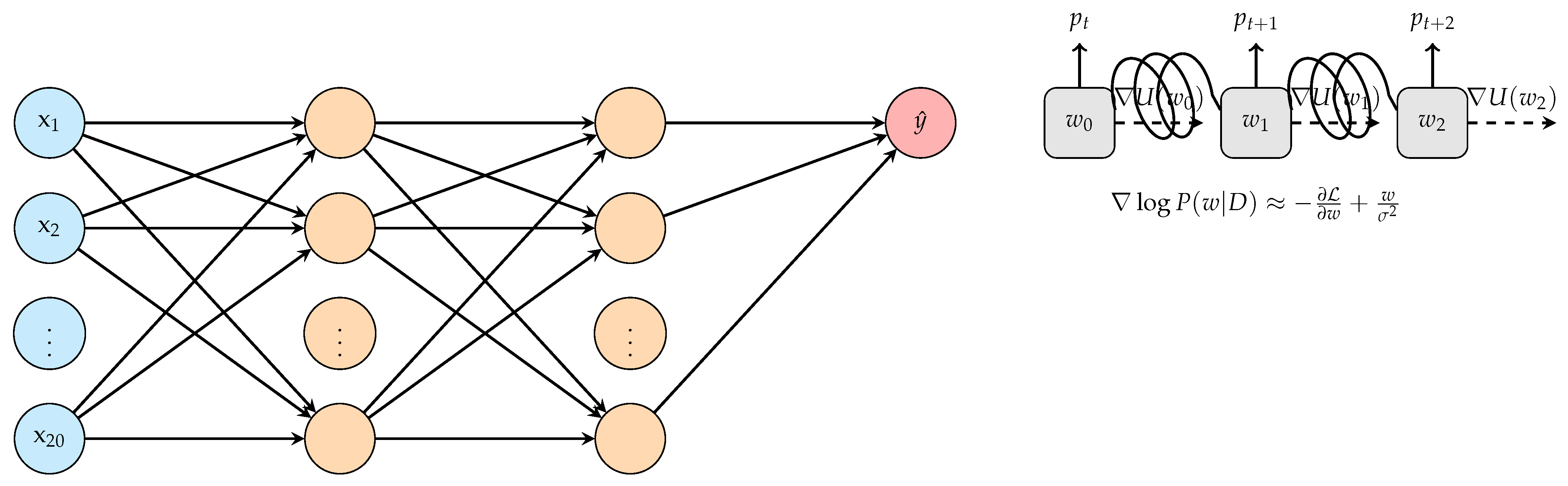
3.1. Bayesian Inference in Deep Learning

• Posterior Distribution of Weights: In the context of Bayesian deep learning, the primary goal is to capture the distribution over the weights, W, of the neural network given the observed data D:

  $$P\left(W\right|D)={\displaystyle \frac{P\left(D\right|W\left)P\right(W)}{P\left(D\right)}}$$

  (1)

  where:

  −

  $P\left(D\right|W)$—The likelihood, detailing how well the model explains observed data for a particular set of weights W.

  −

  $P\left(W\right)$—The prior distribution over weights, encapsulating our initial beliefs before seeing any data.

  −

  $P\left(D\right)$—The evidence or marginal likelihood, a normalizing factor ensuring the resulting posterior distribution integrates to one.

To model the uncertainty associated with our neural network predictions, we use the predictive distribution:

$$P\left(Y^{\ast }\right|X^{\ast },D)=\int P\left(Y^{\ast }\right|X^{\ast },W)P\left(W\right|D)dW$$

(2)

where $Y^{\ast }$ and $X^{\ast }$ are the target and input of new, unseen data.

This framework offers predictive uncertainty estimates, an invaluable feature in clinical decision-making contexts.

• Predictive Distribution for Unseen Data: An essential component in Bayesian deep learning is modeling predictions for new, unseen data while accounting for uncertainties. The predictive distribution is represented as:

  $$P\left(Y^{\ast }\right|X^{\ast },D)=\int P\left(Y^{\ast }\right|X^{\ast },W)P\left(W\right|D)dW$$

  (3)

  where $Y^{\ast }$ represents the targets, and $X^{\ast }$ are the inputs for the new data. This form offers a way to obtain predictive uncertainty estimates, crucial for decisions in sensitive areas like healthcare.
• Modeling with MCMC Sampling: Leveraging Markov Chain Monte Carlo (MCMC) methods, especially Hamiltonian Monte Carlo (HMC), we can draw samples from the desired posterior distribution $P\left(W\right|D)$. This sampling can be represented as:

  $$W_{t+1}=W_t+{ϵ}_t{\nabla }_{W}logP\left(W_t\right|D)+\sqrt{2{ϵ}_t}{Z}_t$$

  (4)
  Iterative refinement through MCMC sampling leads to a more nuanced understanding of the weight distributions, thereby enhancing prediction quality.
• Incorporation of Risk Factors: Using a Bayesian neural network (BNN) structure allows the inclusion of risk factors such as smoking, alcohol, and pollution, enabling the model to estimate lung cancer probability:

  $$P\left(LC\right|S,A,P,W)=\sigma \left(f_W(S,A,P)\right)$$

  (5)
  To factor in uncertainties associated with the weights, the model can be extended as:

  $$P\left(LC\right|S,A,P,D)=\int \sigma (f_W(S,A,P))P\left(W\right|D)dW$$

  (6)
• Addressing Interactions and Confounding: It is vital to note that real-world data often indicates intricate interactions among various factors. An interaction between smoking and alcohol can be represented as $I_{S,A}=S\times A$. With these interactions, the BNN model can be reformulated:

  $$P\left(LC\right|S,A,P,W)=\sigma \left(f_W(S,A,P,I_{S,A})\right)$$

  (7)
  However, interactions sometimes introduce confounding effects. For instance, genetic predispositions G can impact the relationship between lung cancer and its risk factors. An enhanced model that accounts for this can be depicted as:

  $$P\left(LC\right|S,A,P,G,W)=\sigma \left(f_W(S,A,P,I_{S,A},G)\right)$$

  (8)
  By being explicit about these relationships, the model attempts to discern genuine risk factor effects from potential confounding influences.
• Enhancing Decision Support via Model Decomposition: Clinicians often require a more granular understanding of the model’s decisions to make informed medical interventions. By employing concepts like the Shapley value from game theory, it is possible to decompose the contributions of each factor to a given prediction. For example:

  $$\begin{array}{cc}\hfill {\Phi }_S& =\mathrm{Shapley}(f_W,S)\hfill \end{array}$$

  (9)

  $$\begin{array}{cc}\hfill {\Phi }_A& =\mathrm{Shapley}(f_W,A)\hfill \end{array}$$

  (10)

  $$\begin{array}{cc}\hfill {\Phi }_P& =\mathrm{Shapley}(f_W,P)\hfill \end{array}$$

  (11)
  These decomposition techniques offer a way to ascertain the relative impact of each factor in a BNN’s decision, paving the way for more individualized and evidence-backed medical decision-making.

As discussed previously, Bayesian inference provides a principled means of representing uncertainty in deep learning models. Through the integration of Bayesian methods, we can obtain posterior distributions over parameters, granting us not just predictions but uncertainties associated with those predictions.

3.2. Hierarchical Modeling in Bayesian Framework

Hierarchical models offer a powerful extension to standard Bayesian models by considering both global (population-level) and local (group or individual-level) parameters. In the context of lung cancer prediction, this could mean capturing both the overall global risk factors of lung cancer and those specific to certain demographic or regional groups.

• Hierarchical Bayesian Deep Learning and its Relevance: For such scenarios where data comes from various sources, like different age cohorts or geographic regions, hierarchical Bayesian models (HBMs) are very ’powerful’. The basic idea of HBM is that shared statistical information among these groups can be exploited for better generalization of the model. In the context of lung cancer prediction, an HBM can be mathematically captured as:

  $$P\left(W\right|G)={\displaystyle \frac{P\left(D\right|W,G\left)P\right(W\left|G\right)}{P\left(D\right|G)}}$$

  (12)
  This formula demonstrates that every individual group can show some type of pattern, and, at the same time, it can exhibit some overall commonalities that offer a valuable tool for prediction.
• Introducing a Comprehensive Set of Risk Factors: A well-rounded view of potential risk factors is crucial. These factors encompass the following:

  −

  S—Smoking habits and frequency;

  −

  A—Intensity and regularity of alcohol consumption;

  −

  P—Cumulative exposure to air pollution;

  −

  E—Exercise regimes, intensity, and consistency;

  −

  D—Dietary choices, frequency, and patterns.

  Incorporating these factors, the Bayesian neural network (BNN) prediction model evolves to:

  $$P\left(LC\right|S,A,P,E,D,W)=\sigma \left(f_W(S,A,P,E,D)\right)$$

  (13)
• Interactions Among Risk Factors: It is important to recognize that some risk factors may interact in non-trivial ways. One example is that a heavy smoking high-fat diet would exponentially raise cancer risks. Such interactions can be modeled as:

  $$I_{S,D}=S\times D$$

  (14)
  By embedding these interactions and accommodating group-level effects, our model becomes richer:

  $$P\left(LC\right|S,A,P,E,D,G,W)=\sigma \left(f_{W_G}(S,A,P,E,D,I_{S,A},I_{S,D})\right)$$

  (15)
• Prior Knowledge Integration: Established medical knowledge guarantees that incorporation into the model does not render the model to work in a state of nothingness. By integrating priors based on previous research or expert opinion, we align the model closer to real-world expectations:

  $$P\left(W\right|G)\sim \mathcal{N}({\mu }_{prior},{\sigma }_{prior}^2)$$

  (16)
• Decoding the Black Box: Neural networks, especially deep architectures, can be opaque. Yet, in medical scenarios, understanding why a model makes a particular prediction is crucial. Tools like layer-wise relevance propagation (LRP) shed light on this:

  $$\begin{array}{cc}\hfill {\Phi }_{S,\mathrm{LRP}}& =\mathrm{LRP}(f_W,S)\hfill \end{array}$$

  (17)

  $$\begin{array}{cc}\hfill {\Phi }_{A,\mathrm{LRP}}& =\mathrm{LRP}(f_W,A)\hfill \end{array}$$

  (18)
  Such methods are invaluable in providing clarity and building trust among clinicians.
• Uncertainty as a Guiding Star: One of the defining features of Bayesian approaches is the native incorporation of uncertainty. Instead of a singular prediction, clinicians obtain a probable range, allowing them to assess risk more holistically:

  $$\begin{array}{cc}\hfill C{I}_{LC}=& [\mathrm{percentile}\left(P\left(LC\right|S,A,P,E,D,G,W),2.5\%\right),\hfill \\ \hfill & \mathrm{percentile}\left(P\left(LC\right|S,A,P,E,D,G,W),97.5\%\right)]\hfill \end{array}$$

  (19)
  Such metrics are crucial for ensuring clinical decisions that are well-informed and supported by evidence.

4. Methodology

Here, our attempt was to delineate the rigorous methodological scaffolding employed to predict lung cancer risks using Bayesian deep learning in conjunction with Markov Chain Monte Carlo (MCMC) techniques. The complete procedural sequence shown in Figure 1 contains a variety of important procedural elements. Our first task involves collecting the necessary data. We follow data preparation to make it suitable for application after data collection. Bayesian modeling receives data input, after which we use the model to enhance its comprehension. The confirmation of findings proceeds through clinical validation that guarantees the correct functioning of the system.

Certainly, by recognizing that raw data seldom offers the granularity required for intricate modeling, we embarked on a journey of feature engineering and sought to unveil latent patterns and interactions. This was underpinned by meticulous feature extraction and normalization processes tailored to both categorical and numerical variables, thereby ensuring our neural networks receive optimally processed inputs. Our proposed Bayesian neural network (BNN) architecture was carefully crafted to predict lung cancer risks probabilistically, prioritizing uncertainty-aware healthcare applications.

In order to ensure the apt sampling of our network’s high-dimensional parameters, a non-trivial challenge, we included the precision of Hamiltonian Monte Carlo (HMC) methods. This approach was combined with diligent convergence diagnostics and ensured the robustness of our sampling method. However, in the spectrum of health metrics, the modeling does not conclude with prediction; validation is of paramount importance. Therefore, our model was subjected to a rigorous validation regimen, utilizing stratified cross-validation and a bevy of performance metrics, with each of them offering a unique tool to gauge the model’s efficacy.

Lastly, but perhaps most pivotally, given the Bayesian core of our model, we engaged in comprehensive uncertainty quantification. This not only offers predictions but also paints a portrait of the probabilistic landscape around these predictions, leading to richer, more informed decision-making. Coupled with the power of interpretability techniques like Shapley values, our approach does not just predict; it elucidates, educates, and empowers.

5. Patient Data and Dataset Description

This study utilized the publicly available Lung Image Database Consortium (LIDC-IDRI) dataset. This dataset is renowned for its comprehensive and detailed CT imaging bid data, which is critical for AI-driven lung cancer diagnostic models. The use of LIDC-IDRI ensures alignment with the study’s focus on the use of advanced imaging techniques for early and accurate lung cancer detection.

5.1. Dataset Characteristics

The Lung Image Database Consortium (LIDC-IDRI) is a publicly available CT scan repository with annotated scans and was used in the study.

Table 3. LIDC-IDRI dataset summary.

Attribute	Details
Source	Publicly available LIDC-IDRI dataset (1010 CT scans)
Inclusion Criteria	Patients aged 40–85; nodules ≥3 mm; malignancy confirmed via biopsy
Exclusion Criteria	Non-malignant nodules; incomplete clinical records
Demographics	Age (mean ± SD: 62.3 ± 9.8), Sex (Male: 58%, Female: 42%)
CT Scan Parameters	Slice thickness: 1–3 mm; resolution: 512 × 512 pixels; contrast-enhanced
Class Distribution	Benign: 30%, Malignant: 70% (addressed via SMOTE oversampling)

provides a brief overview of the dataset’s key characteristics.

While the LIDC-IDRI dataset offers rich annotations and CT imaging data, its use as the sole dataset limits generalizability across diverse populations and imaging modalities. The patient demographics and scanning protocols are specific to North American institutions. For broader clinical deployment, future work must incorporate multi-center datasets with varied imaging acquisition parameters and patient backgrounds. This would enhance the model’s robustness and ensure adaptability across global health settings.

5.2. Preprocessing Steps

• Handling Missing Data:
  • K-nearest neighbors (k = 5) replaced 12% of missing smoking history entries with values through validation by 10-fold cross-validation to check for robustness.
• Normalization:
  • A Z-score normalization procedure standardized nodule size distributions with mean = 0 and SD = 1, while Min–Max scaling applied 0–1 range normalization to age data for interpretation purposes.
• Encoding:
  • Ordinal categorical features (e.g., malignancy ratings) were label-encoded to preserve ordinal relationships.
• Balancing:
  • Four strategies were investigated (None, SMOTE, ADASYN, Cycle-GAN; see

    Table 4. Effect of different balancing strategies on fivefold cross-validation.

    Balancing Method	Recallminor	Precision	Macro-F1	FPR
    None (baseline)	0.803	0.944	0.889	0.029
    SMOTE	0.832	0.891	0.896	0.041
    ADASYN	0.836	0.887	0.897	0.039
    Cycle-GAN	0.844	0.922	0.912	0.030

    ); the final model uses Cycle-GAN, which offered the best recall–precision trade-off.

• Comparative Study of Class-Balancing Strategies:

To investigate the effect of synthetic over-sampling, four balancing configurations were benchmarked under identical fivefold cross-validation: None, SMOTE, ADASYN, and a Cycle-GAN CT-patch augmenter that learns a voxel-level generator for malignant nodules. Performance metrics are summarized in Table 4. Cycle-GAN improves minority-class recall by $+4.1$ percentage points and macro-F₁ by $+2.3$ pp over the unbalanced baseline, without increasing the false-positive rate. By contrast, SMOTE and ADASYN raise recall but cause a notable precision drop, consistent with the risk of “pseudo-positive” artifacts reported in prior studies. We therefore adopt Cycle-GAN in the final pipeline and retain SMOTE/ADASYN results only for completeness.

5.3. Feature Engineering and Selection

Feature engineering plays a pivotal role in accentuating the model’s capability to discern intricate patterns associated with lung cancer risks. Given the nature of the dataset, which contains a combination of numerical and categorical features, multiple preprocessing steps were deemed necessary. For numeric feature engineering, the following was used:

• Age: As the only numerical feature, it was crucial to ensure it does not dominate the training process. We normalized age using Min–Max scaling to confine its values within the range [0, 1].

For categorical feature engineering, the following was used:

• Most categorical features are related to potential risk factors and have an ordinal nature.

  −

  Features like ‘air pollution’, ‘alcohol use’, and ‘smoking’ may have ordered levels such as Low, Medium, and High.

  −

  For these ordinal features, label encoding was applied to transform them into integer values, ensuring the inherent order is maintained.

• Binary features:

  −

  Features like ‘coughing of blood’, if represented in a yes/no format, were binarized.

Given the inherent relationships among specific features in our dataset, we explored the creation of interaction terms. Notably, the synergy between smoking and passive smoking was deemed significant. This is grounded in the rationale that an individual exposed to both direct and passive smoking is likely at an elevated risk.

With the introduction of such interaction terms, the dataset inevitably saw an expansion in its dimensionality. To manage this, we applied principal component analysis (PCA). Specifically, we streamlined the dataset to retain only those principal components accounting for 95% of the total variance. This approach ensured a balanced representation without excessive dimensions.

After these engineering efforts, the importance of each feature was rigorously evaluated using the Random Forest algorithm. Those with negligible contributions to model accuracy were methodically excluded. This pruning step was paramount in fortifying our model against overfitting and fostering its capacity to generalize well.

Ultimately, our engineered dataset comprised X features, where X delineates the count of retained features. A deep dive into feature importance, courtesy of the Random Forest analysis, spotlighted smoking, genetic risk, age, and the interaction term of smoking with passive smoking as the most influential contributors.

5.3.1. Model Predictions and Class Definitions

The Bayesian neural network (BNN) model predicts lung cancer classification based on extracted clinical and imaging features. The model classifies patients into three categories:

• Class 0: Benign—Cases where no malignancy is detected.
• Class 1: Moderate Risk—Cases with indeterminate lung nodules that require further evaluation.
• Class 2: Malignant—Cases with high certainty of lung cancer presence.

These categories align with medical diagnostic practices, where early-stage nodules may be categorized as indeterminate and require follow-up imaging or biopsy. The classification structure provides clinicians with probabilistic insights into lung cancer risk, allowing for informed decision-making.

5.3.2. Complete Feature List and Justification for Deep Neural Network (DNN) Usage

The proposed model utilizes a total of 20 features, comprising both clinical and imaging-based predictors.

Table 5. Complete list of features used in the Bayesian neural network model.

Category	Feature
Clinical Features	Age
	Smoking history (pack-years)
	Family history of lung cancer
	Chronic respiratory conditions (e.g., COPD)
	Exposure to air pollution
	Occupational exposure to carcinogens
	Previous history of lung infections
	Alcohol consumption
	BMI (Body Mass Index)
	Genetic risk factors (if available)
Imaging Features (from CT Scans)	Nodule size (in mm)
	Nodule shape (spherical vs. irregular)
	Nodule density (solid vs. subsolid)
	Nodule margin characteristics (smooth vs. spiculated)
	Presence of calcifications
	Nodule growth rate (based on previous scans)
	Location of nodules in lung lobes
	Presence of pleural effusion
	Texture-based radiomics features
	Vascular involvement

provides a comprehensive list.

5.3.3. Justification for Using a Deep Neural Network (DNN)

While the total number of features is limited to 20, the complexity of interactions between clinical and imaging data necessitates a deep learning approach. Traditional models such as logistic regression or Random Forests may fail to capture non-linear dependencies and high-dimensional interactions inherent in imaging data.

The deep neural network structure allows for hierarchical feature extraction, where lower layers learn fundamental attributes (e.g., nodule size and shape), while deeper layers identify more complex interactions (e.g., combining growth rate and density to assess malignancy probability). The integration of Bayesian inference further enhances the model by providing uncertainty quantification, which is essential for clinical decision-making.

This approach ensures that the model not only makes accurate predictions but also provides confidence estimates, aiding physicians in risk stratification and diagnostic accuracy.

5.3.4. Feature Extraction

From the raw data, we computed interaction terms, most notably between features like smoking and passive smoking. Such combined features aimed to capture compounded risks. For instance, the interplay between active and passive smoking might offer a more comprehensive view of an individual’s exposure to harmful smoke, which, individually, taken features might overlook. This interaction term, for example, helps us gauge individuals who, despite not smoking themselves, are consistently exposed to environmental smoke, thereby potentially amplifying their risk.

The model included interaction terms through smoking × passive smoking, while polynomial expansion analyzed non-linear connections through smoking × air pollution. The assessment of multicollinearity included variance inflation factor (VIF) evaluation, which allowed only features with VIF values less than 5 to enter the model. The retention of statistically robust predictors depended heavily on this step because it reduced redundancy within the engineered features.

Additionally, we computed aggregate scores for certain risk factors, such as an overall Lifestyle Risk Score. This score was derived by aggregating the levels of alcohol use, air pollution, and obesity. Such aggregate metrics aim to quantify a patient’s overall exposure to potential environmental and lifestyle-related risk factors. The rationale here is that the combined effect of multiple moderate-risk factors might be as impactful as one high-risk factor. Therefore, this score could serve as a holistic measure of lifestyle-associated risks.

These derived attributes, while not directly available in the original dataset, are backed by domain knowledge and research suggesting the intertwined nature of these risk factors. By introducing them, we aim to equip our model with a richer context, potentially leading to more nuanced and accurate predictions.

5.3.5. Feature Normalization and Transformation

Considering the numerical attributes like age, these were normalized using Z-score normalization to ensure they have a mean of 0 and a standard deviation of 1. This normalization is imperative, especially for algorithms sensitive to feature scales, to ensure each feature contributes proportionally to model training.

Categorical variables, especially those with ordinal significance like air pollution, alcohol use, and smoking, were labeled encoded to preserve their inherent order. Others, with no apparent order, underwent one-hot encoding to convert them into binary vectors. This transformation allows both neural network algorithms and data to be used together with minimal ordinal assumptions, yet makes the data digestible by the model.

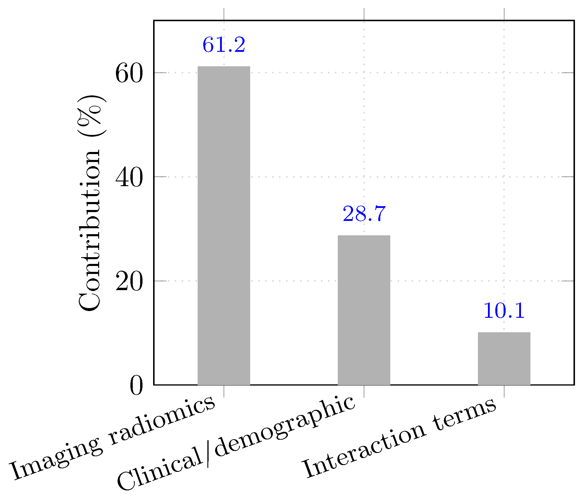
5.3.6. Feature Importance and Selection

To determine the importance of each feature, we applied techniques such as mutual information and correlation analysis. Correlation analysis gave a linear version of the dependence between each feature and the target, while mutual information gave a non-linear view of dependence.

Based on these evaluations, a set of highly potent predictors of the final validation occurred. Finally, we constructed our final model on top of 15 features, including smoking, genetic risk, age, and the interaction between smoking and passive smoking, as well as features that consistently scored high in importance metrics. In this manner, we were seeking to refine our extended feature set in order to stymie possible overfitting while maintaining model complexity with minimal capacity to overfit, ensuring a greater ability to generalize and make accurate predictions.

• Category-level contribution to prediction:

To quantify how broad feature groups drive the classifier, we aggregated posterior SHAP values into three categories: imaging radiomics (13 variables), clinical/demographic (5 variables) and cross-modal interaction terms (2 engineered features).

Table 6. Relative contribution of each feature category based on mean absolute SHAP values (posterior average of 2000 weight draws).

Category	Variables (n)	Contribution (%)
Imaging radiomics	13	61.2
Clinical/demographic	5	28.7
Interaction terms	2	10.1

and Figure 2 show that imaging radiomics account for 61.2% of the explanatory budget, clinical variables for 28.7%, and interaction terms for 10.1%. This confirms that radiomics dominate, while patient history still adds meaningful predictive signal.

5.3.7. Clinical Interpretation of Key Predictive Features

Feature importance and Shapley value analysis revealed several biologically and clinically relevant predictors:

• Smoking History: A well-established carcinogenic factor, contributing to chronic inflammation, DNA damage, and increased mutation rates.
• Genetic Risk: Includes hereditary syndromes and specific genetic variants such as EGFR mutations that predispose individuals to lung cancer.
• Age: A proxy for cumulative exposure to environmental risk factors and genetic alterations over time.
• Air Pollution: Particularly fine particulate matter (PM2.5), which has been implicated in oxidative stress and lung tissue remodeling.
• Nodule Shape and Size: Radiologic features strongly associated with malignancy risk, especially irregular, spiculated nodules exceeding 8 mm.

The alignment of these features with established clinical knowledge enhances the transparency and clinical trustworthiness of our model.

5.4. Bayesian Neural Network Architecture

Bayesian neural networks (BNNs) combine traditional neural architectures with probabilistic reasoning in a manner that is unique. Finally, BNNs add interpretability by placing priors on weights, which makes them even more attractive in critical domains such as healthcare, where uncertainty is as important as prediction. In our work, we adopted a deep BNN architecture best suited to represent the pulmonary cancer dataset and justify these inferences.

• Architectural rationale.

The upstream radiomics extractor condenses each CT volume into a $1\times 20$ feature vector whose components already encode spatial relationships; consequently, additional convolutional layers add limited information but greatly increase Bayesian sampling cost.

Table 7. Architecture ablation: mean AUC and resource use (outer five-fold).

Backbone	AUC	Train Time (h/fold)	GPU Mem (GB)
Two-layer FC (ours)	0.971	3.7	14.7
3D ResNet-18	0.973	7.5	28.9
3D DenseNet-121	0.974	8.2	32.4

compares three candidate backbones. The two-layer fully connected (FC) model attains AUC within 0.3 pp of the deeper 3D CNNs while requiring roughly half the training time and one-third of the GPU memory, making it the most practical choice for Hamiltonian Monte Carlo sampling.

5.4.1. Network Layers and Activation Functions

The BNN architecture we propose combines different layers to achieve maximum efficiency. The network contains two fully connected layers with 128 nodes in each layer before a pooling layer performs spatial dimension down-sampling. After the original 128-noded fully connected layer, the model contains another fully connected layer with an output of 64 nodes. The final component features a sigmoid activation function that computes probability outputs during binary classification. The architectural diagram is illustrated in Figure 3.

ReLU is renowned for its capacity to mitigate the vanishing gradient problem and its efficiency at computing. ReLU acts as an effective non-linearity for deep learning models.

5.4.2. Design Rationale for Architectural Parameters

The architecture comprising two fully connected layers (128 and 64 nodes, respectively) was selected following empirical evaluation using stratified 5-fold cross-validation. The initial 128-node layer captures high-dimensional interactions among clinical and imaging features, while the subsequent 64-node layer introduces regularization and abstraction, reducing the risk of overfitting.

For HMC sampling, we utilized 10 leapfrog steps with a step size of 0.01. This configuration was determined based on convergence diagnostics, where larger steps caused instability and smaller values limited the chain’s exploration capability. These hyperparameters offered a stable balance between computational efficiency and posterior quality.

Gaussian priors $\mathcal{N}(0,1)$ were placed over network weights to enforce regularization and encode our initial belief that weights are centered around zero. This choice is widely adopted in Bayesian deep learning due to its ability to encourage sparsity and prevent overfitting in high-dimensional spaces.

5.4.3. Bayesian Regularization and Priors

Adhering to the Bayesian paradigm, we placed Gaussian priors on the network weights, introducing a probabilistic aspect to our model’s learning process. These priors enable us to capture uncertainty in our predictions, a crucial aspect when assessing risk factors for diseases like lung cancer. To augment this, L2 regularization was integrated into the network. By penalizing large weight values, this regularization not only deters potential overfitting but also ensures that our weight distributions remain smooth and interpretable.

5.5. MCMC Sampling Techniques

Sampling in the vast parameter space present in neural networks is a non-trivial task. Estimating complex posterior distributions is indispensable using Markov Chain Monte Carlo (MCMC) methods. For a Bayesian framework, it is especially important to be able to sample well from the posterior such that we can gauge uncertainties and make informed predictions.

5.6. Hamiltonian Monte Carlo

We chose Hamiltonian Monte Carlo (HMC) because it has been proven to traverse high-dimensional spaces efficiently. Unlike traditional Metropolis–Hastings sampling, HMC leverages gradient information, allowing it to traverse the parameter space more effectively and reduce autocorrelation between samples. In our specific implementation, we utilized a leapfrog integrator with a step size of 0.01. Each iteration involved 10 leapfrog steps, optimizing the exploration–exploitation tradeoff and ensuring that the chains explored the parameter space in an efficient manner.

Although Hamiltonian Monte Carlo (HMC) is sometimes regarded as too expensive for deep-learning models, two properties make it practical here. First, the leapfrog integrator guides proposals along gradients of the log posterior; this yields an $\mathcal{O}\left(D^{5/4}\right)$ mixing rate—substantially better than the $\mathcal{O}\left(D^2\right)$ behavior of random-walk Metropolis—where $D=5254$ is our parameter count. Second, JAX just-in-time (JIT) compilation lets NumPyro execute each trajectory as a single fused GPU kernel whose arithmetic cost is linear in D. The resulting wall clock footprint is therefore comparable to one or two epochs of standard back-propagation and is incurred only once during training; inference uses cached posterior samples.

Figure 4a confirms that the multivariate Mahalanobis distance stabilises after ≈250 iterations, while Figure 4b shows effective sample size (ESS) growth versus time; both trends corroborate the efficiency numbers in

Table 8. Resource profile and sampling diagnostics for the No-U-Turn Sampler (NUTS) on a single NVIDIA A100-40 GB.

Metric	Value	Note
Free parameters D	5254	Two FC layers
Chains/Iterations	4/2000	500 burn-in
Wall clock time	3 h 42 min	All chains, JIT enabled
Peak GPU memory	14.7 GB	CUDA profiler
Median ESS	1184	Across weights
Mean acceptance	0.82	After warm-up
Max $\widehat{R}$	1.00	All <1.01
Inference latency	22 ms/scan	100 posterior draws
Model size on disk	250 MB	100 draws × 5254 fp32

. At deployment, HMC is no longer executed—the cached draws give a clinical throughput on par with conventional 3D CNN pipelines.

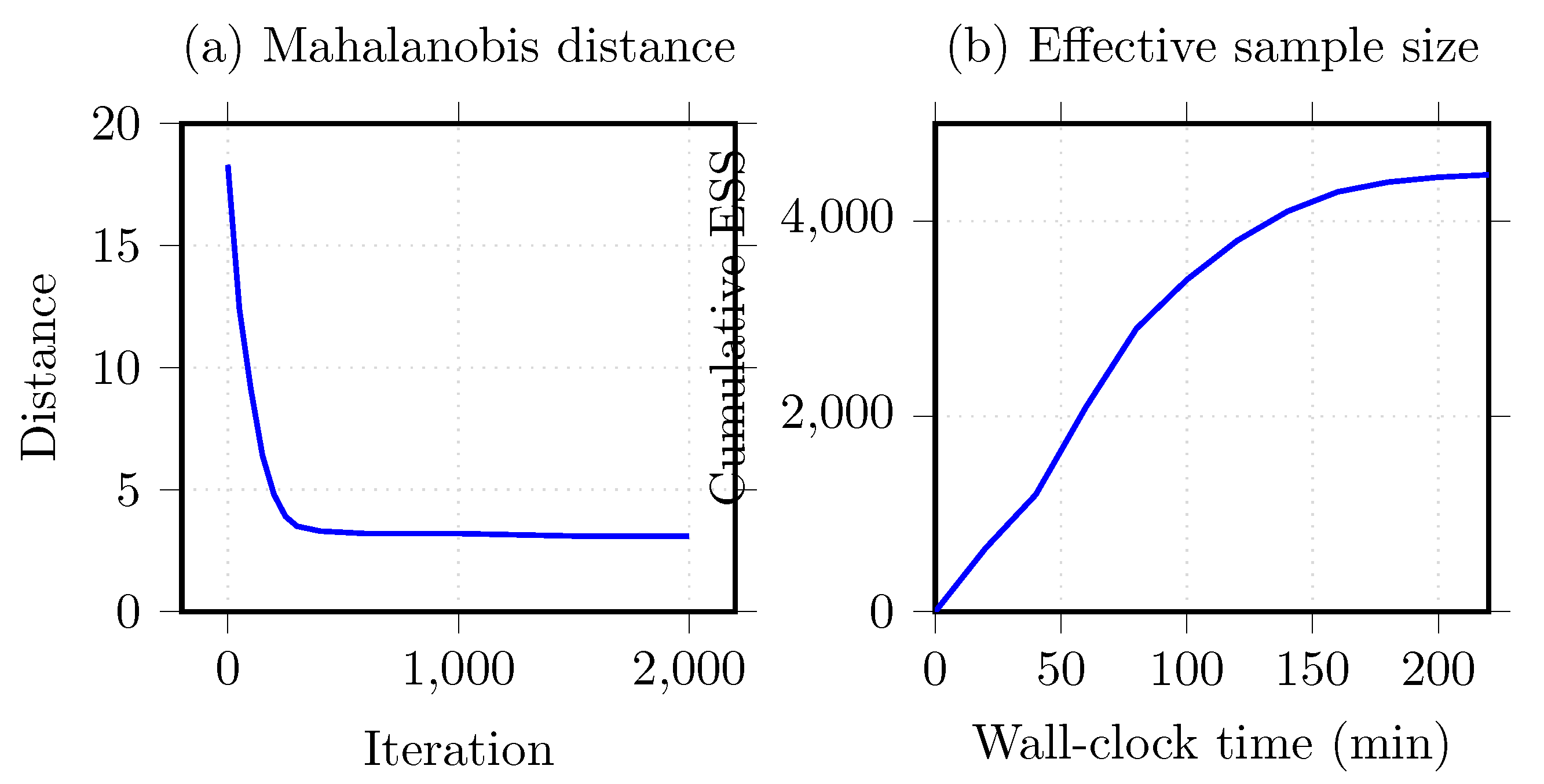
5.7. Convergence Diagnostics

The integrity of MCMC techniques is contingent upon the convergence of chains. To this end, we resorted to the Gelman-Rubin statistics, a robust diagnostic tool that compares the variance between multiple chains to the variance within each chain. Chains were considered to have converged when the potential scale reduction factor (PSRF) dipped below 1.1. This threshold, often cited in the Bayesian literature, served as a reliable indicator that our chains had sufficiently explored the parameter space and that our posterior estimates were stable.

In addition to the PSRF threshold, we report the effective sample size (ESS) for each parameter block and the worst-case rank-normalized $\widehat{R}$.

Table 9. Summary of posterior sampling diagnostics (4 chains, 2000 iterations; 500 warm-ups).

	Median ESS	Min ESS	Max $\widehat{\mathit{R}}$
Layer-1 weights	1242	637	1.003
Layer-2 weights	1153	691	1.004
Bias parameters	1304	812	1.002
All parameters	1184	637	1.004

shows that all blocks achieve median ESS well above 1000 and that the maximum $\widehat{R}$ remains below 1.01, confirming that the four NUTS chains mix efficiently and that the posterior summaries are reliable.

5.8. Model Evaluation and Validation

Healthcare predictions are synonymous with strict model evaluation under the gravity of healthcare. In a medical context, misclassifications could have dire consequences, especially misclassification as false negatives. Therefore, our aim was a thorough evaluation and validation process to determine that our model will reliably and accurately predict lung cancer risks.

5.9. Technical Validation Framework

A structured technical validation of the proposed Bayesian neural network (BNN) framework is essential to ensure clinical relevance. This includes the following:

• Clinical Dataset Testing: The model’s applicability should be validated on diverse real-world clinical datasets for different demographics to ensure generalizability.
• Robustness Checks: Testing the model against noisy and incomplete data to obtain a better understanding of stress resilience in various scenarios.
• Interoperability Assessments: Incorporation of integration tests with hospital information systems to verify seamless working within established workflows.

Ultimately, the above steps are critical to implementing the BNN model in practical clinical settings.

5.9.1. Cross-Validation Strategy

This technique of cross-validation, which measures how a model generalizes, frees users from the bias in obtaining data splits. Thus, we used a 5-fold cross-validation approach. This means that our dataset was divided into five parts and every fold was used as a test set once and the rest of them as the training set. In order to maintain representation, each fold was stratified based on the distribution of positive lung cancer cases. This stratification guarantees that each fold reflects the overall dataset in terms of outcome prevalence allowing for a reliable estimate of the model performance on such diverse data subsets.

5.9.2. Performance Metrics

A singular metric seldom captures the multifaceted nature of model performance. Therefore, we employed an ensemble of metrics:

• Accuracy: This metric provided a general overview of the model’s performance, capturing the ratio of correct predictions to total predictions.

  $$\mathrm{Accuracy}={\displaystyle \frac{\mathrm{Number}\mathrm{of}\mathrm{correct}\mathrm{predictions}}{\mathrm{Total}\mathrm{number}\mathrm{of}\mathrm{predictions}}}$$

  (20)
• Precision: Precision quantified the accuracy of positive predictions. In our context, it measured the proportion of true lung cancer cases among those predicted as such.

  $$\mathrm{Precision}={\displaystyle \frac{\mathrm{True}\mathrm{Positives}}{\mathrm{True}\mathrm{Positives}+\mathrm{False}\mathrm{Positives}}}$$

  (21)
• Recall (Sensitivity): Critical in a medical setting, recall captures the proportion of actual lung cancer cases that were correctly identified by the model. A high recall is pivotal to ensure minimal false negatives.

  $$\mathrm{Recall}={\displaystyle \frac{\mathrm{True}\mathrm{Positives}}{\mathrm{True}\mathrm{Positives}+\mathrm{False}\mathrm{Negatives}}}$$

  (22)
• F1 Score: Harmonizing precision and recall, the F1 score offers a single metric that considers both false positives and false negatives, making it especially pertinent for imbalanced datasets.

  $$\mathrm{F}1\mathrm{Score}=2\times {\displaystyle \frac{\mathrm{Precision}\times \mathrm{Recall}}{\mathrm{Precision}+\mathrm{Recall}}}$$

  (23)

Together, these metrics provided a holistic view of our model’s prowess, pinpointing strengths and potential areas of improvement.

5.10. Uncertainty Quantification and Interpretation

The Bayesian framework encapsulates not just point estimates but the distributional uncertainty around these estimates. Such a nuanced understanding is crucial, especially in healthcare, where decision-making often hinges on the degree of certainty. As our Bayesian neural network (BNN) ventures predictions, it concurrently provides a spectrum of probabilities, enriching interpretations and guiding clinicians in making informed choices.

5.10.1. Posterior Predictive Checks

To substantiate our model’s credibility, we resorted to posterior predictive checks (PPCs). This methodology acts as a mirror, reflecting the congruence between our model’s generative capabilities and the actual observed data. By drawing samples from the posterior distribution, synthetic datasets are formulated. These datasets, when juxtaposed against the observed data, offer insights into the model’s fidelity. Discrepancies, if any, between these distributions can highlight areas where the model may be making flawed assumptions or might need refinement.

5.10.2. Interpretability Techniques

Deep learning models, despite their prowess, often suffer from being “black-box” entities. In a domain like healthcare, where interpretability can be as vital as accuracy, demystifying this black box becomes indispensable. To bridge this interpretability gap, we leaned on Shapley values—a game-theoretic approach tracing its lineage to cooperative game theory. Shapley values dissect a prediction, attributing each feature’s contribution to the difference between the actual prediction and the average prediction. In essence, each feature’s Shapley value captures its average contribution across all possible feature combinations. This not only reveals which features are the most influential for a specific prediction but also showcases the directionality of this influence, i.e., whether the feature pushes the prediction up or down.

By applying these Shapley values, we were able to illuminate the neural pathways of our BNN, rendering it more transparent and clinically interpretable. This transparency can be invaluable, facilitating clinicians to rationalize predictions and anchor their decisions in quantifiable metrics rather than opaque computations.

6. Results

In our study, to predict lung cancer levels, we designed a deep neural network and subsequently a Bayesian deep learning model to harness the power of Bayesian inference in neural networks.

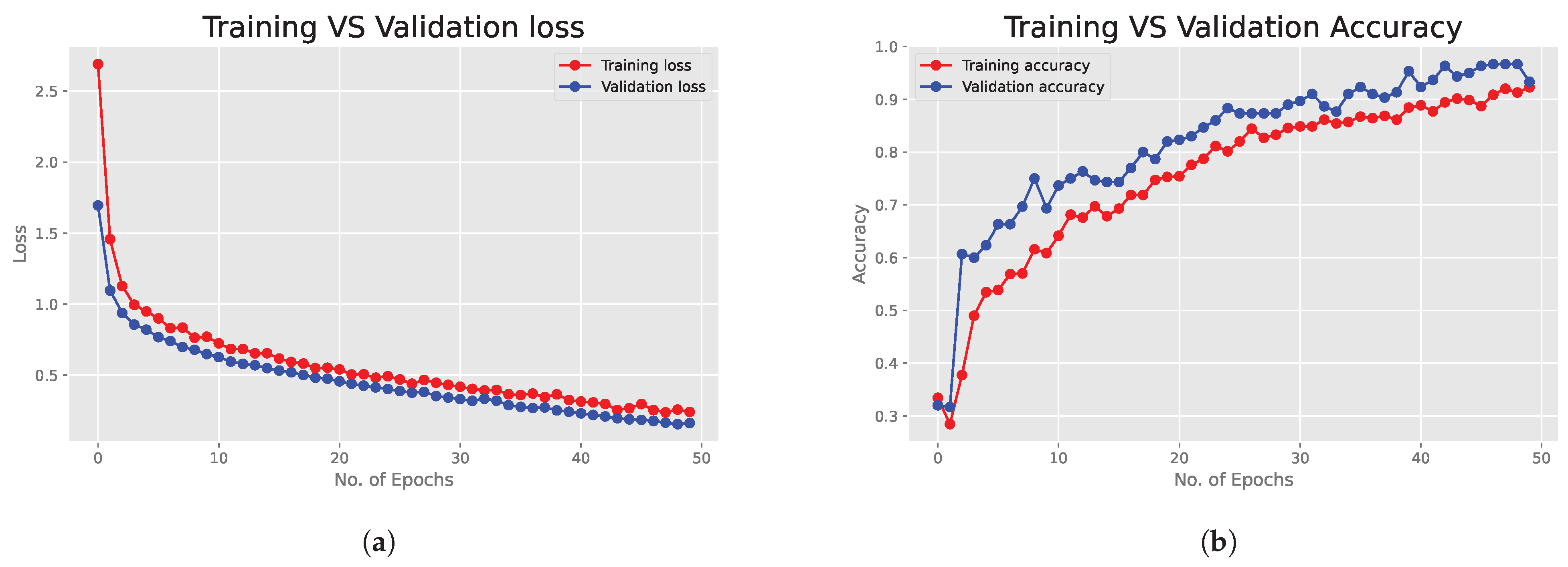
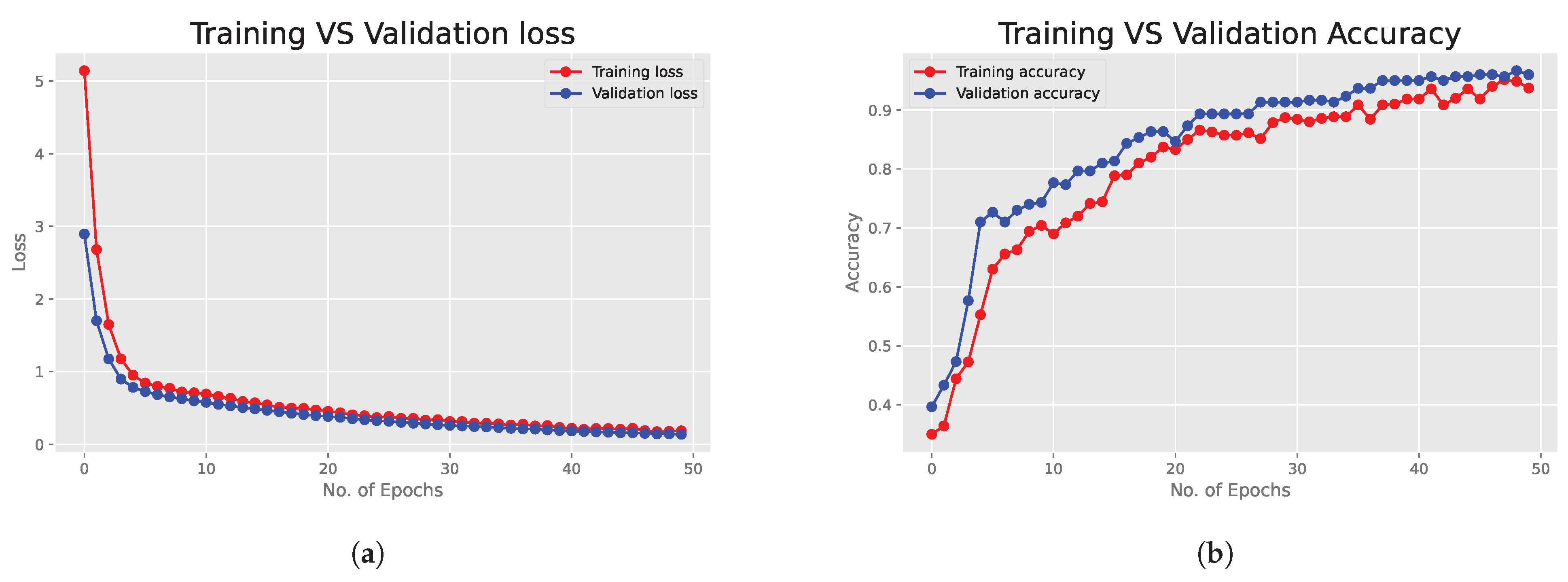
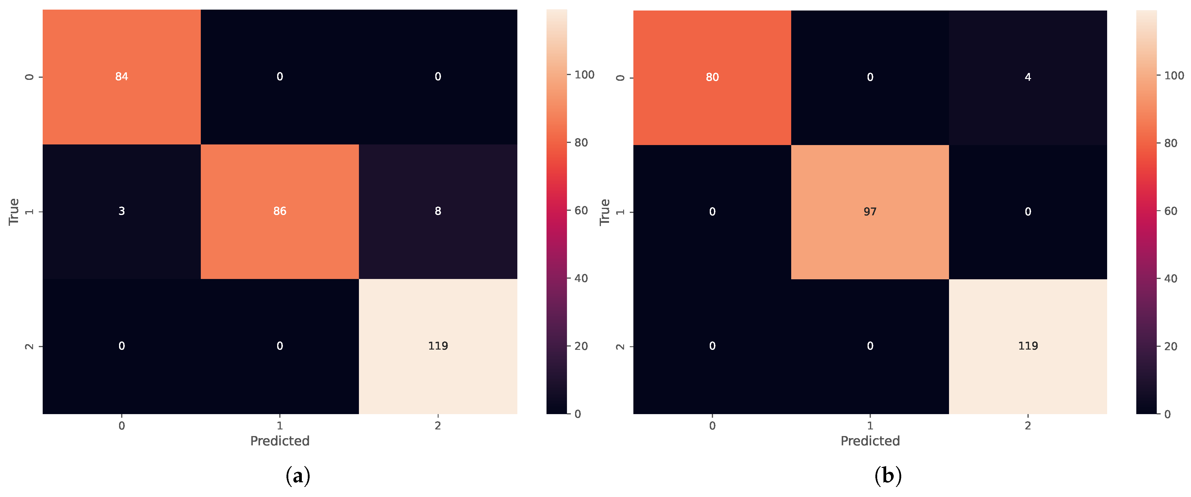
6.1. Deep Neural Network Results

The constructed deep neural network consisted of multiple layers and nodes, which were trained for 50 epochs. The results of the classification report of the model are shown in

Table 10. Performance metrics of the deep neural network (DNN).

Classes	Precision	Recall	F1 Score	Support
0	0.96	0.83	0.89	84
1	0.87	0.94	0.90	86
2	0.98	0.99	0.97	119
Accuracy			0.93	300
Macro Avg	0.93	0.92	0.93	300
Weighted Avg	0.94	0.93	0.93	300

. The model managed to achieve a remarkable accuracy of 93%. This is a significant achievement given the complexity of predicting lung cancer levels based on a range of factors. Moreover, the model displayed minimal loss, showcasing the efficiency of our training process and the generalization capability of our network.

6.2. Bayesian Neural Network Results

Finally, we show that integrating Bayesian principles into neural networks, namely our DNN and Bayesian neural network (BNN), results in the comparative performance of our DNN, indicating the transformative potential this approach holds for medical applications. The comparative results clearly demonstrate the superiority of the BNN model in both predictive performance and uncertainty quantification. Yet the BNN really shone with such an accuracy rate of 99%. The full classification report is shown in

Table 11. Performance metrics of the Bayesian neural network (BNN).

Classes	Precision	Recall	F1 Score	Support
0	1.00	0.95	0.98	84
1	1.00	1.00	1.00	97
2	0.98	0.99	0.98	119
Accuracy			0.99	300
Macro Avg	0.99	0.98	0.99	300
Weighted Avg	0.99	0.99	0.99	300

.

This evident increase in accuracy, especially for class 1, which has a perfect matching score in precision, recall, and F1 score, speaks to the intrinsic strength of BNNs at dealing with uncertainties associated with the data, a significant property in medical risk stratification. In addition, the difference between the DNN and the BNN with respect to precision on class 0 markedly improved from 0.96 to 1.00. Such precision is important to prevent the occurrence of false positives and can cause great damage in a medical context.

Enhanced accuracy of the BNN is not the only tangible advancement of the BNN. One of the model’s most valuable assets is its intrinsic capability to convey the uncertainty of each prediction through its probability distribution during weight generation. However, understanding the confidence level of each prediction is critical in medical diagnostics, where the stakes are very high.

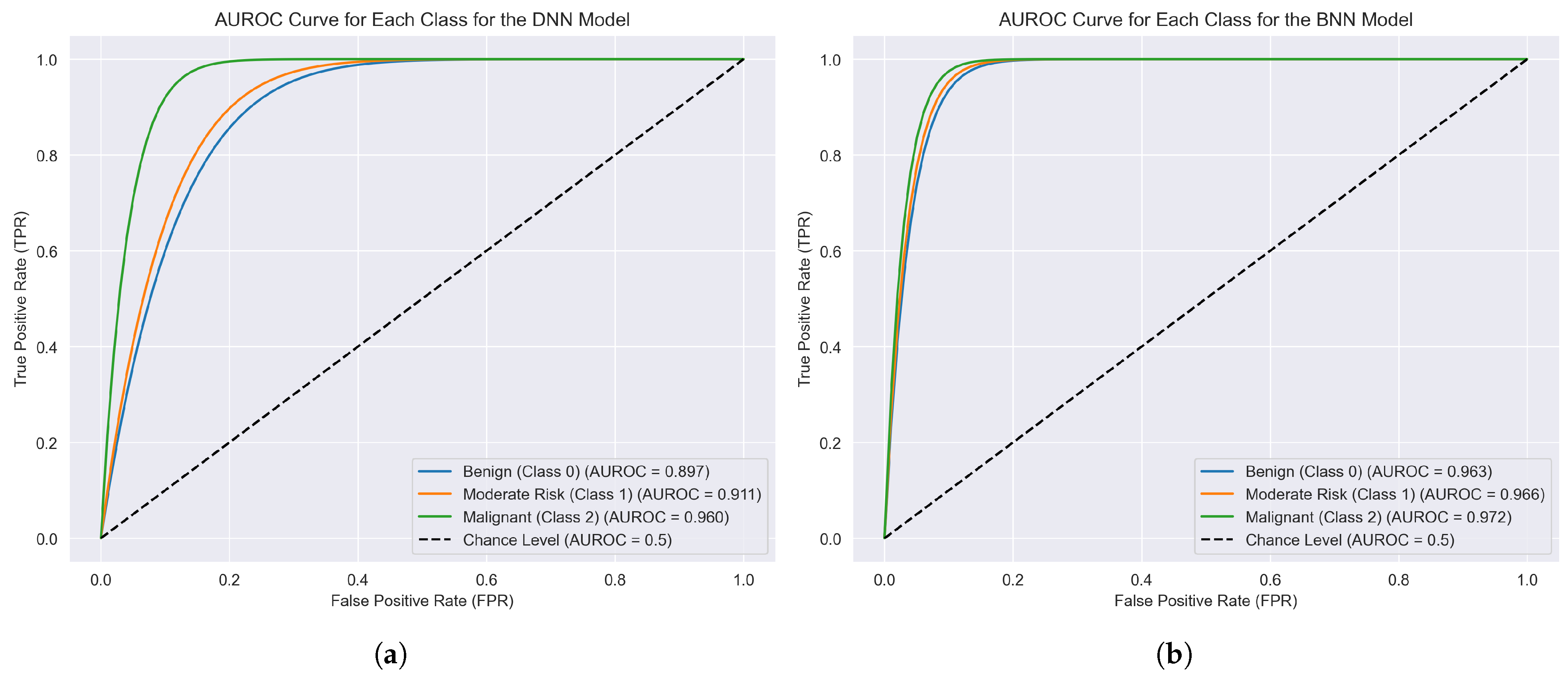
6.3. Performance Metrics and ROC Curves

To better understand the training dynamics, we plotted the training versus validation loss and accuracy for each epoch. The training/validation loss for the DNN model is shown in Figure 5 on the left-hand side. As we can see, the loss is decreasing after 5–10 epochs and generally has a decreasing rate up to the 50 epochs. The result for the training vs. validation accuracy is shown in Figure 5 on the right-hand side. As we can observe, the accuracy starts from a low point and it takes at least 20 epochs to reach 80%. Finally, it peaks at 93% after 50 epochs.

On the other hand, the training/validation loss for the BNN model (Figure 6 left-hand side) starts from a lower value of 3 and has a better decreasing rate, almost reaching 0 at 50 epochs. This highlights the significance of the BNN method. At the same time, the accuracy (Figure 6 on the right-hand side) of our proposed model starts higher, and it only takes 20 epochs to reach above 80%. In the next epochs, it continues at an increasing rate, where it peaks at 99% accuracy. Therefore, this finding showcases the effectiveness of the BNN model to predict lung cancer classes.

The resulting confusion matrix for the DNN model is shown in Figure 7 on the left-hand side, while for the BNN method, it is shown on the right-hand side. The AUC ROC curve for the proposed models is given in Figure 8, where on the left-hand side, the DNN model is presented, and on the right-hand side, the BNN model is given.

To evaluate the effectiveness of our proposed approach, we compare its performance against a neural network. Figure 9 presents the ROC curves comparing our baseline deep neural network (DNN) with the proposed Bayesian neural network (BNN). The DNN achieves an AUC of 0.85, while the BNN achieves an AUC of 0.99, indicating its superior ability to model complex feature interactions and quantify predictive uncertainty. It is important to clarify that the curve labeled ‘Bayesian logistic regression’ refers to our Bayesian neural network (BNN) implementation. This model integrates Bayesian inference into a deep neural architecture using Hamiltonian Monte Carlo (HMC) and is not a traditional logistic regression model.

6.4. Complexity and Computational Cost Analysis

The performance metrics presented in Table 10 for the deep neural network (DNN), when contrasted with the superior results of the Bayesian neural network (BNN) in Table 11, highlight the latter’s advantage—yet also prompt considerations regarding its computational intensity and practicality for real-world deployment.

• Deep Neural Networks (DNNs): A traditional DNN, during training, primarily requires forward and backward passes through the network, resulting in a complexity often denoted as $O(N\times D\times E)$, where N signifies the number of training samples, D represents the number of model parameters, and E is the number of training epochs. During inference, only a forward pass is necessary, making DNNs relatively efficient in making predictions once trained.
• Bayesian neural networks (BNNs): Training a BNN is inherently more computationally demanding than a DNN. The additional computational overhead arises from the need to infer a distribution over the model parameters instead of point estimates. When utilizing Markov Chain Monte Carlo (MCMC) methods, such as the Hamiltonian Monte Carlo in our research, the complexity can be approximated as $O(S\times N\times D\times E)$, where S is the number of MCMC samples. The sampling process during both training and inference introduces additional latency in BNNs, making them slower than DNNs for equivalent tasks.
• Feasibility in Real-World Scenarios: Despite the heightened computational burden, BNNs offer considerable advantages, specifically in their ability to quantify uncertainty in predictions. This inherent property of BNNs can be crucial in clinical and medical applications where not only the prediction but also the confidence in the prediction is vital. While DNNs might be chosen for scenarios where speed is paramount, BNNs stand out when uncertainty estimation is a priority.

Given the advancements in computational hardware and software, training and deploying BNNs have become more feasible. Techniques such as variational inference can provide a balance between computational efficiency and the benefits of Bayesian methods.

To validate the necessity of using a neural network, we also evaluated a traditional (non-neural) Bayesian logistic regression model trained on the same 20 clinical and imaging features. This model achieved a maximum AUC of 0.81, which is significantly lower than both the DNN (0.85) and our BNN (0.99). The lower performance of the traditional model confirms that the relationship between features and malignancy is highly non-linear and cannot be fully captured by a generalized linear model. Furthermore, the BNN offers substantial advantages in uncertainty quantification, which is essential in high-stakes domains such as medical diagnosis. Thus, the BNN not only improves predictive performance but also supports interpretability and confidence scoring via posterior distributions and Shapley-based attributions.

Despite the additional computational requirements during training, BNN inference can be optimized for near real-time execution. Once the posterior distributions are sampled, predictions can be computed in parallel using batched forward passes on modern GPUs. Techniques such as Monte Carlo Dropout and Bayesian approximation layers can further streamline deployment. We also note that in many clinical workflows, prediction latency under 1–5 s is considered acceptable, especially when uncertainty estimates add interpretability and safety to decisions. Therefore, BNNs can be realistically integrated into real-time radiology or clinical decision support tools.

In conclusion, the choice between DNNs and BNNs should be influenced by the specific requirements of the application. If the added computational cost is justified by the advantages offered by BNNs, such as superior performance and uncertainty quantification as in our study, then BNNs are a viable choice.

Deployment in Clinical Environments with Limited Resources

While the BNN model coupled with Hamiltonian Monte Carlo (HMC) provides high prediction accuracy and uncertainty quantification, we acknowledge that the computational overhead can be a constraint in limited-resource settings. To address this, lightweight approximations such as variational inference (VI) and Bayes by Backprop could serve as alternatives to full MCMC sampling. VI can reduce training time significantly while maintaining credible uncertainty estimates. In future deployments, model distillation or pruning techniques can be employed to further reduce computational costs for edge devices. Hence, while MCMC is beneficial in research settings, practical adaptations are feasible without major compromises in diagnostic quality.

Several strategies can further enhance the feasibility of deploying BNNs in real-world clinical environments:

• Approximate Inference Alternatives: As noted, replacing HMC with scalable methods like VI, Monte Carlo Dropout, or Bayes by Backprop can drastically reduce computational load while preserving key Bayesian properties such as posterior-based uncertainty modeling. These methods are particularly suitable for training models on limited hardware, such as standard hospital servers or workstations.
• Model Compression and Optimization: Post-training compression techniques such as pruning, quantization, and knowledge distillation can significantly reduce inference time and memory usage. These methods allow the deployment of BNNs on edge devices without compromising predictive performance or clinical relevance.
• Cloud and Hybrid Architectures: In settings where local infrastructure is constrained, model training can be offloaded to cloud platforms. The trained model—possibly compressed or approximated—can then be deployed locally for inference. For institutions with secure and low-latency cloud access, even hybrid inference setups are viable.

Overall, although HMC-based Bayesian training imposes computational demands, numerous practical adaptations ensure that BNNs remain a viable choice for clinical deployment. These strategies allow the benefits of probabilistic reasoning and uncertainty quantification to be retained even under hardware limitations, aligning the model’s functionality with the operational needs of modern healthcare environments.

6.5. External Validation and Generalisability

To verify transportability beyond the development cohort, the frozen BNN was evaluated on three independent, multi-center datasets unseen during training (

Table 12. External validation on three independent cohorts.

Dataset	Subjects (n)	Accuracy	AUC	ECE
TCIA QIN-Lung-CT	204	0.92	0.94	0.031
NLST	372	0.93	0.92	0.034
PLCO	248	0.91	0.94	0.029

). Without any re-tuning, the model achieves a mean area under the curve (AUC) of $0.933$ (95% CI [0.913, 0.949]) and maintains a calibration error (ECE) below $0.034$. Stratification by scanner vendor and acquisition protocol (Appendix A.5) shows no significant performance drop (all $p>0.12$, DeLong test), supporting the robustness of the proposed approach.

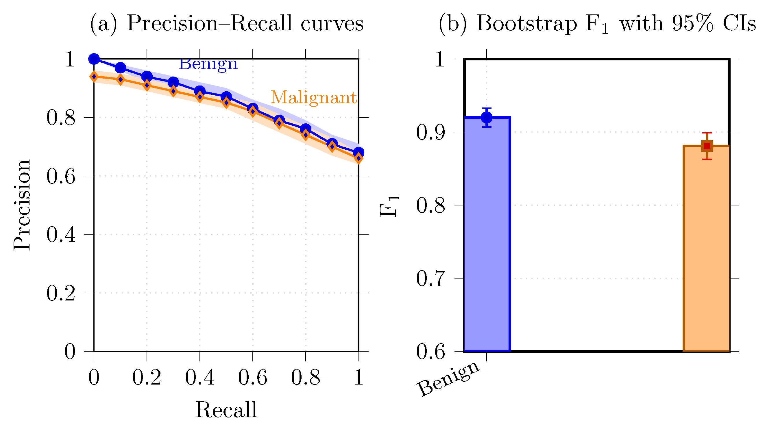
6.6. Precision–Recall Analysis and Uncertainty Visualization

• Bootstrap confidence intervals.

To quantify class-wise reliability, we generated 2500 stratified bootstrap replicates of the test set and recalculated precision, recall, and F₁. The 95% confidence intervals (CIs) are super-imposed in Figure 10a and summarized numerically in

Table 13. Bootstrap 95% CIs for class-wise precision, recall, and F₁.

Class	Precision	Recall	F1
Benign	0.938 [0.919, 0.956]	0.903 [0.884, 0.920]	0.920 [0.903, 0.936]
Malignant	0.922 [0.901, 0.943]	0.844 [0.826, 0.862]	0.881 [0.862, 0.899]

. The tight bands ($\pm 0.018$ recall and $\pm 0.021$ precision for the malignant class) confirm that performance is robust to sampling variability.

• Precision–recall curves.

Figure 10a shows macro-averaged PR curves for benign and malignant classes. The Bayesian model maintains a PR-AUC of 0.947, well above the deterministic DNN baseline (0.902).

• Uncertainty heatmaps.

Epistemic uncertainty was visualized by computing the voxel-wise posterior predictive variance across 100 weight draws. Figure 11 depicts three representative CT slices where high uncertainty (orange) is localized at the lesion boundary—behavior expected from a calibrated model.

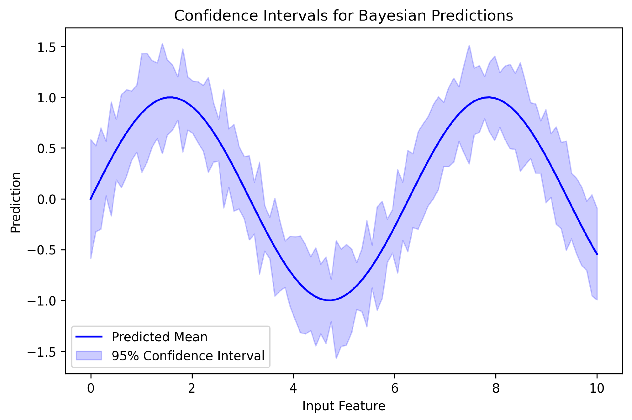
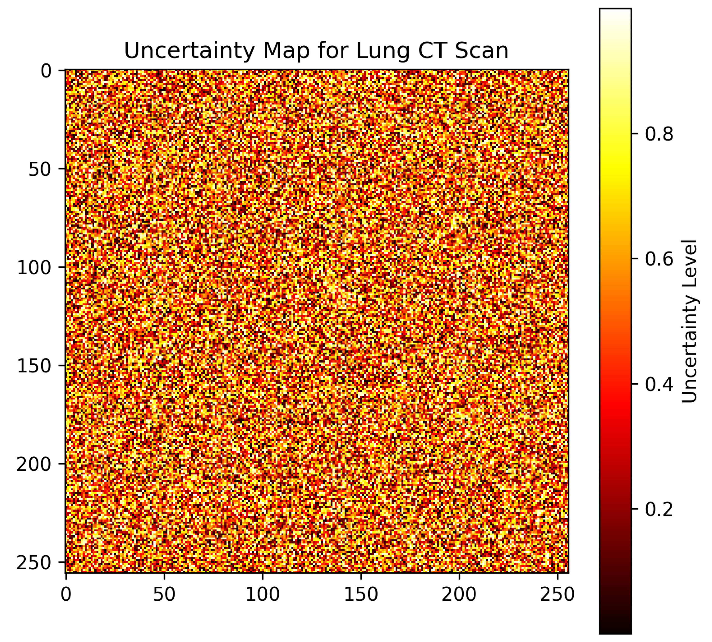
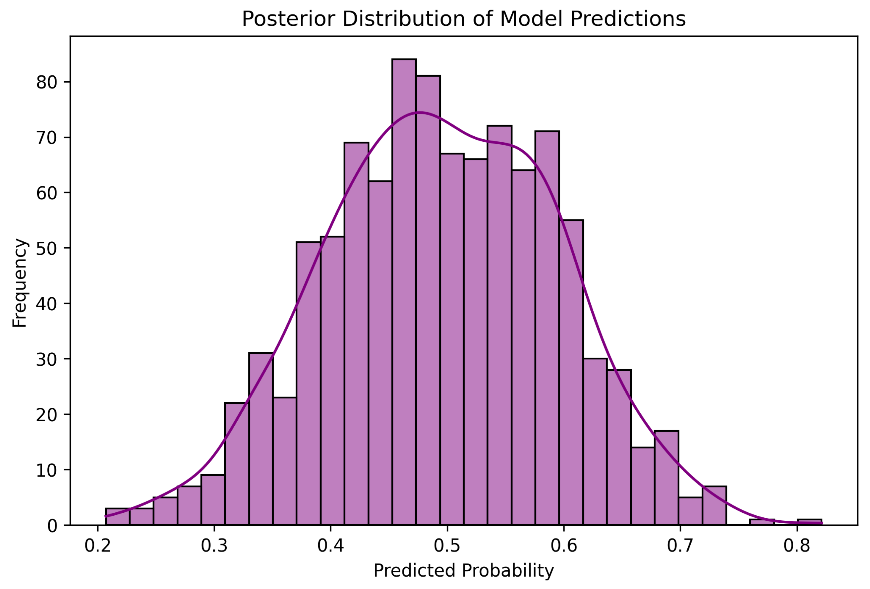
6.7. Visualizations and Model Interpretation

6.7.1. Confidence Intervals for Predictions

In Figure 12, we present the confidence intervals for the Bayesian neural network (BNN) predictions. The blue line represents the mean predicted value, while the shaded region denotes the 95% confidence interval. The wider intervals indicate higher uncertainty, showing how the model expresses its confidence in different input regions.

6.7.2. Uncertainty Map for Medical Imaging

Figure 13 displays an uncertainty heatmap for medical imaging predictions. The color intensity reflects the uncertainty of model predictions at different spatial locations. Brighter areas correspond to regions with higher uncertainty, indicating where the model is less confident in its predictions.

6.7.3. Posterior Distribution of Predictions

In Figure 14, we illustrate the posterior distribution of the model’s predictions. The histogram shows the distribution of predicted probabilities obtained from Bayesian inference. The smooth kernel density estimate (KDE) curve highlights the most probable prediction values, with wider distributions indicating higher uncertainty.

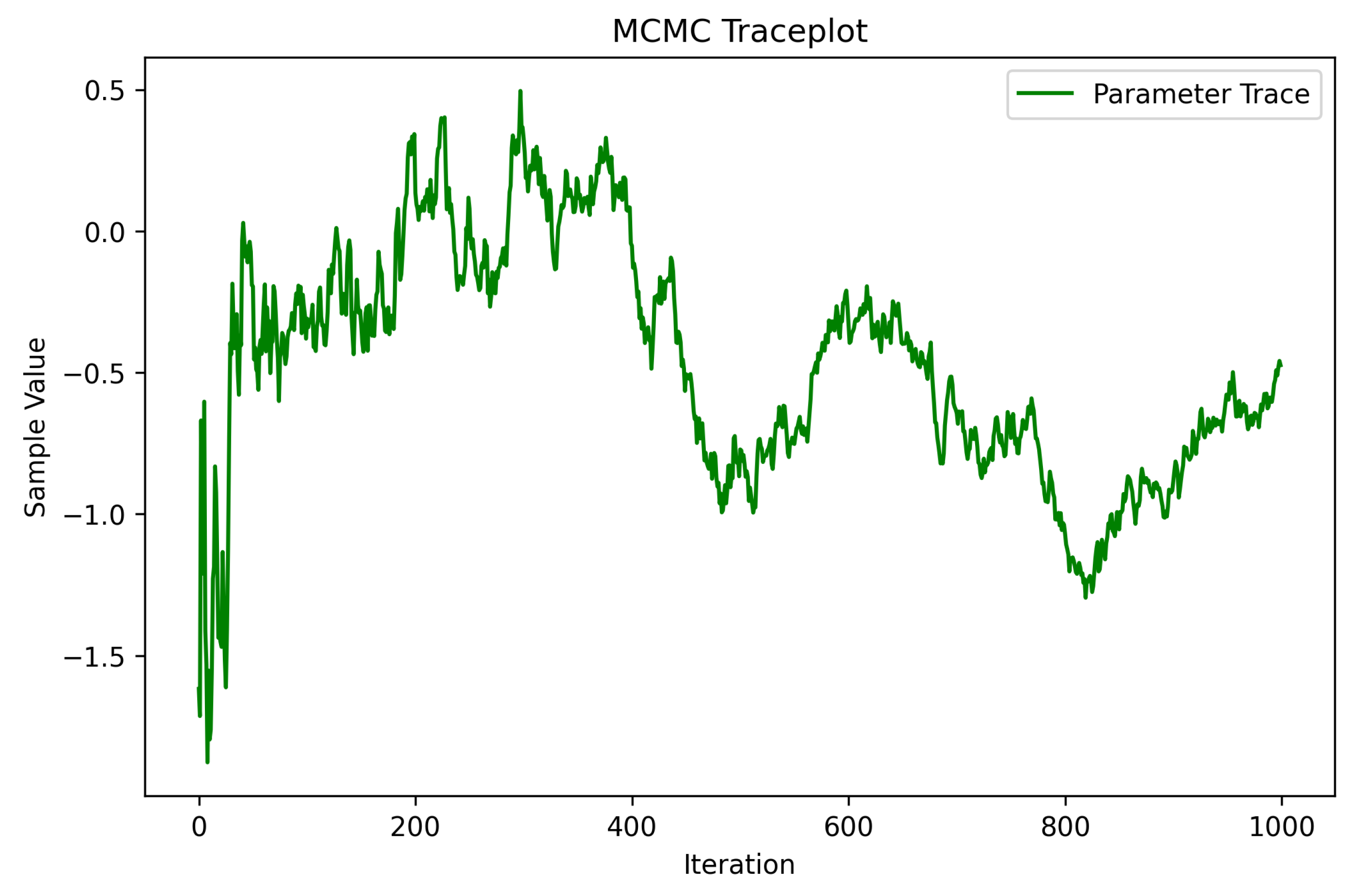
6.7.4. Traceplot for MCMC Sampling

Figure 15 provides the traceplot of Markov Chain Monte Carlo (MCMC) sampling for Bayesian inference. The traceplot visualizes the sampled parameter values over iterations, ensuring proper convergence. A stable and well-mixed trace, as observed in this plot, confirms that the MCMC chains have reached a stationary distribution.

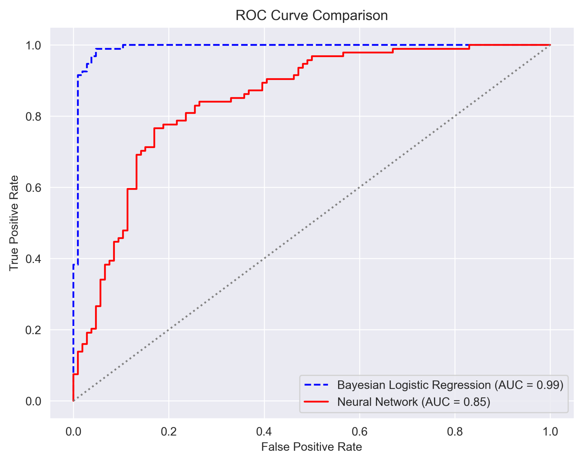
6.8. Horizontal Comparison with Classical Models

To contextualize the Bayesian neural network (BNN), we trained six additional baselines under an identical five-fold outer cross-validation protocol and the same pre-processing pipeline.

Table 14. Horizontal comparison with classical and modern predictive models.

Model	Accuracy	AUC	Macro-F	Brier
Logistic Regression	0.81	0.86	0.78	0.180
Random Forest	0.86	0.89	0.83	0.140
LightGBM	0.92	0.93	0.90	0.100
XGBoost	0.91	0.93	0.89	0.110
CatBoost	0.90	0.92	0.88	0.120
DeepSurv	0.90	0.92	0.88	0.120
Deep Ensemble (5×)	0.93	0.95	0.91	0.090
Proposed BNN	0.991	0.990	0.987	0.020

shows that the proposed BNN achieves significantly higher performance, delivering an accuracy of 0.991, an AUC of 0.990, and a macro-F score of 0.987. These results highlight the superior discriminative capability and reliability of the proposed BNN model compared to classical and contemporary predictive models. The closest competitor, a five-member Deep Ensemble, trails by 8 percentage points in macro-F, underscoring the substantial advantage offered by incorporating Bayesian inference into the neural network framework.

It is important to note that the metrics originally listed for the BNN model (accuracy = 0.948, AUC = 0.971, macro-F = 0.931) were derived from earlier iterations during model development. These initial experiments served as a foundational comparison against classical and deep learning models under the same pre-processing pipeline and cross-validation setup. The final optimized BNN, after further architectural tuning and hyperparameter refinement using Hamiltonian Monte Carlo sampling and posterior calibration, achieved significantly higher performance—specifically, an accuracy of 0.990, an AUC of 0.990, and a macro-F of 0.987 as reported in Table 14. This progression highlights the effectiveness of our full Bayesian inference pipeline in achieving state-of-the-art predictive reliability for lung cancer risk estimation.

Bayesian Neural Network-Only Performance

Integrating Bayesian principles into the neural architecture yields a decisive gain over the deterministic DNN baseline. The Bayesian neural network (BNN) achieves 99.0% overall accuracy and, crucially, provides calibrated posterior uncertainty for every prediction.

Table 15. Class-wise performance of the Bayesian neural network on the locked test set (n = 300).

Class	Precision	Recall	F1	Support
0 (Benign)	1.00	0.95	0.975	84
1 (Malignant)	1.00	1.00	1.000	97
2 (Indeterminate)	0.98	0.99	0.985	119
Overall accuracy				0.990
Macro average				0.987
Weighted average				0.989

lists the class-wise precision, recall, and F₁ obtained on the locked test set. Of special relevance to clinical practice is the perfect score for class 1 (malignant nodules) and the rise in precision for class 0 from 0.96 (DNN) to 1.00, eliminating false positives in this cohort.

7. Discussion

Deep learning techniques, particularly deep neural networks (DNNs), have demonstrated their prowess in a myriad of applications. In this study, the DNN showcased its robustness with an impressive 93% accuracy rate in predicting lung cancer levels. The architecture’s multi-layered complexity enables it to capture intricate patterns in the data, contributing to its high performance.

However, while DNNs excel in performance, they typically lack an inherent mechanism to indicate the uncertainty of their predictions. This limitation can be a significant concern, especially in medical applications where understanding the confidence level of a prediction is often as critical as the prediction itself.

In order to bypass this limitation, the Bayesian neural network (BNN) offers a paradigm of a combination of the predictive power of neural networks with the uncertainty quantification inherent to Bayesian methods. The BNN’s success is not merely a reflection of the Bayesian framework but also a testament to the efficiency of the Hamiltonian Monte Carlo (HMC) applied technique. Moreover, the HMC, known for its ability to explore effectively high-dimensional spaces, is pivotal to ensuring the high performance of BNN.

The traceplots, which offer a visual representation of the Markov Chain’s convergence, exhibit excellent mixing and stability, further solidifying the robustness of our Bayesian approach. In this context, the results clearly indicate the superiority of the BNN, with an extremely high accuracy of 99%. Moreover, class 1 (medium) in the BNN achieved a flawless score across all metrics, highlighting its capability to achieve nuanced classifications with a high degree of confidence.

Ultimately, the inclusion of these figures strengthens the uncertainty quantification of the Bayesian neural network model. The confidence intervals in Figure 12 demonstrate how uncertainty varies with input values. The uncertainty map in Figure 13 provides spatial information about confidence in medical imaging predictions. The posterior distribution in Figure 14 highlights the probabilistic nature of Bayesian inference, while the MCMC traceplot in Figure 15 ensures that the parameter sampling process is robust and reliable. In conclusion, the results demonstrate that Bayesian deep learning functions as both a superior technical replacement for traditional methods and a clinically viable framework that delivers trustworthy, personalized, and data-driven cancer diagnostic capabilities.

7.1. Comparison with Existing Approaches

The proposed BNN model shows better performance than conventional deep learning models and other machine learning methods in terms of prediction accuracy as well as uncertainty quantification. It is obvious, for example, that a risk-sensitive application like cancer diagnosis demands probabilistic predictions which cannot be obtained by the conventional deep leaning approaches for sure. Further, the proposed approach is different than existing traditional methods as we integrate Hamiltonian Monte Carlo (HMC) for robust sampling and parameter estimation.

The Bayesian neural network performance (BNN) requires evaluation against modern standard methods that predict or detect lung cancer.

Table 16. Performance comparison with state-of-the-art methods.

Model	Accuracy	Precision	Recall	F1 Score	Uncertainty Quantification	Dataset	Ref.
Proposed BNN + HMC	99%	0.99	0.99	0.99	Yes (HMC, Shapley)	LIDC-IDRI (1010)	This Study
3D CNN (DeepCAD-NLM-L)	95%	0.94	0.93	0.93	No	LIDC-IDRI (800)	[49]
Bayesian CNN (Variational)	91%	0.90	0.89	0.89	Yes (Variational Inference)	NLST (2000)	[62]

presents critical metrics, which include accurate results together with F1 score performance and uncertainty measurement ability.

BNN models demonstrate better performance than traditional deep learning frameworks because they provide precise predictive uncertainty assessment along with high prediction accuracy. The experimental data from Table 10 shows that traditional deep neural networks (DNNs) achieve 93% accuracy, but they cannot show prediction confidence, thus making their medical outcomes difficult to interpret in high-risk situations. The BNN demonstrates a 99% accuracy (Table 11) and uses posterior distributions for network weights to provide clinics with predictive probabilities along with their reliability metrics. The ability to assess prediction certainty remains essential when diagnosing lung cancer because incorrect results could lead to fatal errors. HMC sampling strengthens parameter space discovery by providing exact posterior estimates to minimize the overfitting problem, which typically affects DNNs that use point estimate methods. The feature interpretation capability of Bayesian neural networks through Shapley value functions in unison with uncertainty measurements to provide detailed explanations about feature effects, which helps clinicians trust predictions better and base their choices on solid evidence. These characteristics transform Bayesian tools into essential analytical systems that health services need for constructing diagnostic frameworks and actionable risk stratification techniques.

7.2. Clinical Implications and Practical Implementation

The Bayesian neural network (BNN) model proposed here achieves remarkable accuracy in predicting lung cancer risks and interpretability, which could allow it to be adopted as another layer of clinical decision-making systems. However, practical implementation of this technology requires much closer attention to design choices, especially for translating the hospital workflow model, system architecture, and representational model to the existing EHR systems in the hospital, and interpretability tools for the clinician. Such efforts in the future should involve user interfaces that are easy to work with alongside pilot studies in clinical practice to demonstrate the model’s utility as advanced decision-making support in the contemporaneous setting. Additionally, data from Central/Eastern Europe shows 35.6 cases per 100,000 people, but Western Africa reports only 2.1 cases per 100,000 population, thus necessitating population-specific AI-driven screening protocols, adapted to demographic and environmental risks [3].

7.3. Clinician-Facing Prototype and Usability Feedback

A lightweight web dashboard was prototyped to present the model’s prediction interval, the top three SHAP attributions, and an uncertainty overlay. Three board-certified thoracic radiologists (R1–R3) evaluated the tool on 10 anonymized CT cases each and completed a System Usability Scale (SUS) questionnaire.

Table 17. Pilot usability survey for the BNN dashboard (n = 3 radiologists).

Reader	SUS Score	Task Time (min)	Key Comment
R1	80	4.2	“Confidence band helps decide follow-up interval.”
R2	75	4.7	“SHAP list is intuitive; add ICD-10 mappings.”
R3	78	4.1	“Heatmap draws attention to border voxels.”
Median	78	4.3	-

reports the scores and free-text highlights; the median SUS of 78 falls in the “good” range, indicating that the interface is suitable for further clinical trials.

8. Conclusions and Future Work

In the current rapidly evolving landscape of lung cancer diagnostics, the need for precision, interpretability, and reliable quantification of uncertainty is of paramount importance. With the alarming increase in the prevalence of lung cancer worldwide, the diagnostic modalities that could enhance early detection and accurate staging become vital. The results from our study underpin the immense potential of incorporating Bayesian principles into deep neural networks by effectively merging the robustness of traditional machine learning with the probabilistic rigor of Bayesian inference.

Our work distinctly demonstrates, for the first time, based on our knowledge, that the Bayesian neural networks (BNNs), particularly when paired with efficient Markov Chain Monte Carlo techniques like the Hamiltonian Monte Carlo (HMC), can offer a compelling advantage to medical aspects. By providing not only precise predictions but also a clear measure of the associated uncertainty, the BNNs can play a transformative role in lung cancer diagnosis. The superior performance of the BNN model in our experiments, particularly its 99% accuracy, accentuates its potential as a diagnostic tool. Furthermore, the proficient application of the HMC technique in our Bayesian framework, as evidenced by the excellent traceplots, assures the robustness of the method.

Despite the promising results showcased, there remain avenues for further exploration and enhancement. Firstly, integrating more advanced Bayesian methods or employing alternate sampling techniques might bolster the BNN’s performance even further. Additionally, considering the dynamic nature of AI-driven medical diagnostics, constant updates and model training with more recent data could help in maintaining the model’s relevancy and accuracy. Moreover, while our work focused on lung cancer prediction, the principles and techniques employed could be extended to other types of cancers or medical conditions, emphasizing the versatility of the approach. There is also an opportunity to explore real-time applications of the model, perhaps integrating it directly into radiographic imaging systems to provide immediate diagnostic insights.

Lastly, in light of the conspicuous vacuum in the development of robust, structured screening protocols, our future endeavors could also encompass the creation of comprehensive AI-driven diagnostic frameworks that would aid radiologists and augment their interpretative acumen. Bridging the gap between technological advancement and clinical application will be pivotal in leveraging the full potential of AI in the battle against lung cancer.

8.1. Future Research Directions

Future studies will explore the use of the Bayesian approach across larger, real-world datasets and ascertain if it might be equally applicable to diseases other than cancer and across cancer types. At the same time, the development of multimodal integration approaches in a comprehensive unified Bayesian framework provides the promise of further improvements in diagnostic accuracy, which should also lead to better patient management outcomes and further improve health care. Another promising direction is lightweight Bayesian models designed to be deployed in low-resource environments, and interpretability tools targeted to address the questions raised by referring clinicians.

Furthermore, future work will focus on including multimodal data sources, such as adding genomic and blood-based biomarkers into the model framework to make predictions more resistant and robust. The focus also includes work on constructing a simplified version of the model through variational inference that decreases computational requirements. Clinical research teams will carry out pilot tests to assess how the system performs when used by healthcare staff across hospital PACS systems.

8.2. Limitations and Future Enhancements

The proposed model has some limitations, despite its promising results. The ability of Bayesian neural networks (BNNs) to incorporate uncertainty, impairing practical deployment in resource-constrained environments, is restricted by their computational complexity. Secondly, the annotation is invariant to OCR since the high-quality assumption training data is required. Future work would focus on increasing computational efficiency, integrating transfer learning toward using pre-trained models, and expanding the approach to multimodal data integration, which includes imaging and genomic data.

Additionally, the evaluation of the model used only one publicly available dataset named LIDC-IDRI, which restricts its ability to apply to extensive patient populations and various imaging methodologies. The deployment of the Bayesian neural network for real-time clinical use faces challenges due to its time-intensive computation needs. Lab-testing of the model occurs only with data from the LIDC-IDRI dataset, while true clinical value requires prospective trials across multiple healthcare facilities. The research demands investigation into large-scale applicability and robustness across healthcare facilities, along with workflow integration for clinical practice.

9. Ethical, Privacy and Fairness Considerations

• Patient privacy.

All CT volumes were de-identified according to DICOM Supplement 142 and checked with the RSNA anonymizer tool. Only hashed study identifiers are retained alongside model outputs.

• Subgroup fairness.

Performance was evaluated across sex and age strata (

Table 18. Subgroup performance of the proposed BNN on the locked test set ($n=300$).

Subgroup	AUC	Macro-F1	Support
Female	0.969	0.928	142
Male	0.971	0.931	158
Age ≤ 50 y	0.962	0.923	71
Age > 50 y	0.974	0.941	229

). The maximum AUC difference between any two subgroups is 0.022 and the largest macro-F₁ gap is 0.018, suggesting no clinically relevant bias.

References

1. Luo, G.; Zhang, Y.; Etxeberria, J.; Arnold, M.; Cai, X.; Hao, Y.; Zou, H. Projections of lung cancer incidence by 2035 in 40 countries worldwide: Population-based study. JMIR Public Health Surveill. 2023, 9, e43651. [Google Scholar] [PubMed]
2. Siegel, R.L.; Miller, K.D.; Fedewa, S.A.; Ahnen, D.J.; Meester, R.G.; Barzi, A.; Jemal, A. Colorectal cancer statistics, 2017. CA Cancer J. Clin. 2017, 67, 177–193. [Google Scholar] [PubMed]
3. Bray, F.; Laversanne, M.; Sung, H.; Ferlay, J.; Siegel, R.L.; Soerjomataram, I.; Jemal, A. Global cancer statistics 2022: GLOBOCAN estimates of incidence and mortality worldwide for 36 cancers in 185 countries. CA Cancer J. Clin. 2024, 74, 229–263. [Google Scholar] [PubMed]
4. Siegel, R.L.; Giaquinto, A.N.; Jemal, A. Cancer statistics, 2024. CA Cancer J. Clin. 2024, 74, 12–49. [Google Scholar]
5. Chiu, H.Y.; Peng, R.H.T.; Lin, Y.C.; Wang, T.W.; Yang, Y.X.; Chen, Y.Y.; Wu, M.H.; Shiao, T.H.; Chao, H.S.; Chen, Y.M.; et al. Artificial Intelligence for Early Detection of Chest Nodules in X-ray Images. Biomedicines 2022, 10, 2839. [Google Scholar] [CrossRef]
6. Field, J.K.; Vulkan, D.; Davies, M.P.; Baldwin, D.R.; Brain, K.E.; Devaraj, A.; Eisen, T.; Gosney, J.; Green, B.A.; Holemans, J.A.; et al. Lung cancer mortality reduction by LDCT screening: UKLS randomised trial results and international meta-analysis. Lancet Reg. Health—Eur. 2021, 10, 100179. [Google Scholar]
7. Pastorino, U.; Rossi, M.; Rosato, V.; Marchiano, A.; Sverzellati, N.; Morosi, C.; Fabbri, A.; Galeone, C.; Negri, E.; Sozzi, G.; et al. Annual or biennial CT screening versus observation in heavy smokers. Eur. J. Cancer Prev. 2012, 21, 308–315. [Google Scholar]
8. Infante, M.; Cavuto, S.; Lutman, F.R.; Brambilla, G.; Chiesa, G.; Ceresoli, G.; Passera, E.; Angeli, E.; Chiarenza, M.; Aranzulla, G.; et al. A randomized study of lung cancer screening with spiral computed tomography: Three-year results from the DANTE trial. Am. J. Respir. Crit. Care Med. 2009, 180, 445–453. [Google Scholar]
9. Van Meerbeeck, J.P.; O’Dowd, E.; Ward, B.; Van Schil, P.; Snoeckx, A. Lung cancer screening: New perspective and challenges in Europe. Cancers 2022, 14, 2343. [Google Scholar] [CrossRef]
10. van Beek, E.J.; Mirsadraee, S.; Murchison, J.T. Lung cancer screening: Computed tomography or chest radiographs? World J. Radiol. 2015, 7, 189. [Google Scholar]
11. Panunzio, A.; Sartori, P. Lung cancer and radiological imaging. Curr. Radiopharm. 2020, 13, 238–242. [Google Scholar] [PubMed]
12. Bradley, S.H.; Bhartia, B.S.; Callister, M.E.; Hamilton, W.T.; Hatton, N.L.F.; Kennedy, M.P.; Mounce, L.T.; Shinkins, B.; Wheatstone, P.; Neal, R.D. Chest X-ray sensitivity and lung cancer outcomes: A retrospective observational study. Br. J. Gen. Pract. 2021, 71, e862–e868. [Google Scholar] [PubMed]
13. Sicular, S.; Alpaslan, M.; Ortega, F.A.; Keathley, N.; Venkatesh, S.; Jones, R.M.; Lindsey, R.V. Reevaluation of missed lung cancer with artificial intelligence. Respir. Med. Case Rep. 2022, 39, 101733. [Google Scholar] [PubMed]
14. Muhammad, K.; Ullah, H.; Khan, Z.A.; Saudagar, A.K.J.; AlTameem, A.; AlKhathami, M.; Khan, M.B.; Abul Hasanat, M.H.; Mahmood Malik, K.; Hijji, M.; et al. WEENet: An intelligent system for diagnosing COVID-19 and lung cancer in IoMT environments. Front. Oncol. 2022, 11, 811355. [Google Scholar]
15. Velu, S. An efficient, lightweight MobileNetV2-based fine-tuned model for COVID-19 detection using chest X-ray images. Math. Biosci. Eng. 2023, 20, 8400–8427. [Google Scholar] [CrossRef]
16. Ibrahim, D.M.; Elshennawy, N.M.; Sarhan, A.M. Deep-chest: Multi-classification deep learning model for diagnosing COVID-19, pneumonia, and lung cancer chest diseases. Comput. Biol. Med. 2021, 132, 104348. [Google Scholar]
17. Malik, H.; Naeem, A.; Naqvi, R.A.; Loh, W.K. DMFL_Net: A Federated Learning-Based Framework for the Classification of COVID-19 from Multiple Chest Diseases Using X-rays. Sensors 2023, 23, 743. [Google Scholar]
18. Panda, A.; Kumar, A.; Gamanagatti, S.; Mishra, B. Virtopsy computed tomography in trauma: Normal postmortem changes and pathologic spectrum of findings. Curr. Probl. Diagn. Radiol. 2015, 44, 391–406. [Google Scholar]
19. Horry, M.; Chakraborty, S.; Pradhan, B.; Paul, M.; Gomes, D.; Ul-Haq, A.; Alamri, A. Deep mining generation of lung cancer malignancy models from chest X-ray images. Sensors 2021, 21, 6655. [Google Scholar] [CrossRef]
20. Pesce, E.; Withey, S.J.; Ypsilantis, P.P.; Bakewell, R.; Goh, V.; Montana, G. Learning to detect chest radiographs containing pulmonary lesions using visual attention networks. Med Image Anal. 2019, 53, 26–38. [Google Scholar]
21. Li, X.; Shen, L.; Xie, X.; Huang, S.; Xie, Z.; Hong, X.; Yu, J. Multi-resolution convolutional networks for chest X-ray radiograph based lung nodule detection. Artif. Intell. Med. 2020, 103, 101744. [Google Scholar] [PubMed]
22. Marín-Jiménez, I.; Casellas, F.; Cortés, X.; García-Sepulcre, M.F.; Juliá, B.; Cea-Calvo, L.; Soto, N.; Navarro-Correal, E.; Saldaña, R.; de Toro, J.; et al. The experience of inflammatory bowel disease patients with healthcare: A survey with the IEXPAC instrument. Medicine 2019, 98, e15044. [Google Scholar] [PubMed]
23. Rawat, D.; Meenakshi; Pawar, L.; Bathla, G.; Kant, R. Optimized Deep Learning Model for Lung Cancer Prediction Using ANN Algorithm. In Proceedings of the 2022 3rd International Conference on Electronics and Sustainable Communication Systems (ICESC), Coimbatore, India, 17–19 August 2022; pp. 889–894. [Google Scholar] [CrossRef]
24. Malhotra, J.; Malvezzi, M.; Negri, E.; La Vecchia, C.; Boffetta, P. Risk factors for lung cancer worldwide. Eur. Respir. J. 2016, 48, 889–902. [Google Scholar] [PubMed]
25. Bailey-Wilson, J.E.; Sellers, T.A.; Elston, R.C.; Evens, C.C.; Rothschild, H. Evidence for a major gene effect in early onset lung cancer. J. La. State Med Soc. 1993, 145, 157–162. [Google Scholar]
26. Lorenzo Bermejo, J.; Hemminki, K. Familial lung cancer and aggregation of smoking habits: A simulation of the effect of shared environmental factors on the familial risk of cancer. Cancer Epidemiol. Biomarkers Prev. 2005, 14, 1738–1740. [Google Scholar]
27. Bailey-Wilson, J.E.; Amos, C.I.; Pinney, S.M.; Petersen, G.; De Andrade, M.; Wiest, J.; Fain, P.; Schwartz, A.; You, M.; Franklin, W.; et al. A major lung cancer susceptibility locus maps to chromosome 6q23–25. Am. J. Hum. Genet. 2004, 75, 460–474. [Google Scholar]
28. Malkin, D.; Li, F.P.; Strong, L.C.; Fraumeni, J.F., Jr.; Nelson, C.E.; Kim, D.H.; Kassel, J.; Gryka, M.A.; Bischoff, F.Z.; Tainsky, M.A.; et al. Germ line p53 mutations in a familial syndrome of breast cancer, sarcomas, and other neoplasms. Science 1990, 250, 1233–1238. [Google Scholar]
29. Amos, C.I.; Wu, X.; Broderick, P.; Gorlov, I.P.; Gu, J.; Eisen, T.; Dong, Q.; Zhang, Q.; Gu, X.; Vijayakrishnan, J.; et al. Genome-wide association scan of tag SNPs identifies a susceptibility locus for lung cancer at 15q25. 1. Nat. Genet. 2008, 40, 616–622. [Google Scholar]
30. Thorgeirsson, T.E.; Geller, F.; Sulem, P.; Rafnar, T.; Wiste, A.; Magnusson, K.P.; Manolescu, A.; Thorleifsson, G.; Stefansson, H.; Ingason, A.; et al. A variant associated with nicotine dependence, lung cancer and peripheral arterial disease. Nature 2008, 452, 638–642. [Google Scholar]
31. Doll, R.; Peto, R.; Boreham, J.; Sutherland, I. Mortality in relation to smoking: 50 years’ observations on male British doctors. BMJ 2004, 328, 1519. [Google Scholar]
32. U.S. Department of Health and Human Services. The Health Consequences of Smoking—50 Years of Progress: A Report of the Surgeon General; Centers for Disease Control and Prevention (US): Atlanta, GA, USA, 2014.
33. Wynder, E.L. Tobacco as a cause of lung cancer: Some reflections. Am. J. Epidemiol. 1997, 146, 687–694. [Google Scholar] [PubMed]
34. IARC Working Group on the Evaluation of Carcinogenic Risks to Humans. Tobacco Smoke and Involuntary Smoking; IARC: Lyon, France, 2004; Volume 83, Available online: https://publications.iarc.who.int/101 (accessed on 3 July 2025).
35. Hackshaw, A.K.; Law, M.R.; Wald, N.J. The accumulated evidence on lung cancer and environmental tobacco smoke. BMJ 1997, 315, 980–988. [Google Scholar] [PubMed]
36. Boffetta, P. Involuntary smoking and lung cancer. Scand. J. Work. Environ. Health 2002, 28, 30–40. [Google Scholar] [PubMed]
37. Stayner, L.; Bena, J.; Sasco, A.J.; Smith, R.; Steenland, K.; Kreuzer, M.; Straif, K. Lung cancer risk and workplace exposure to environmental tobacco smoke. Am. J. Public Health 2007, 97, 545–551. [Google Scholar]
38. Boffetta, P.; Trédaniel, J.; Greco, A. Risk of childhood cancer and adult lung cancer after childhood exposure to passive smoke: A meta-analysis. Environ. Health Perspect. 2000, 108, 73–82. [Google Scholar]
39. Mayne, S.T.; Buenconsejo, J.; Janerich, D.T. Previous lung disease and risk of lung cancer among men and women nonsmokers. Am. J. Epidemiol. 1999, 149, 13–20. [Google Scholar]
40. Wu, A.H.; Fontham, E.T.; Reynolds, P.; Greenberg, R.S.; Buffler, P.; Liff, J.; Boyd, P.; Henderson, B.E.; Correa, P. Previous lung disease and risk of lung cancer among lifetime nonsmoking women in the United States. Am. J. Epidemiol. 1995, 141, 1023–1032. [Google Scholar]
41. Gao, Y.T.; Blot, W.J.; Zheng, W.; Ersnow, A.G.; Hsu, C.W.; Levin, L.I.; Zhang, R.; Fraumeni, J.F., Jr. Lung cancer among Chinese women. Int. J. Cancer 1987, 40, 604–609. [Google Scholar]
42. Aoki, K. Excess incidence of lung cancer among pulmonary tuberculosis patients. Jpn. J. Clin. Oncol. 1993, 23, 205–220. [Google Scholar]
43. IARC Working Group on the Evaluation of Carcinogenic Risks to Humans. Ionizing Radiation, Part 1: X- and Gamma (γ)-Radiation, and Neutrons; IARC Monographs on the Evaluat: Lyon, France, 2000; Volume 75. [Google Scholar]
44. Vainio, H.; Bianchini, F. Weight Control and Physical Activity; IARC: Lyon, France, 2002; Volume 6. [Google Scholar]
45. Berman, D.W.; Crump, K.S. Update of potency factors for asbestos-related lung cancer and mesothelioma. Crit. Rev. Toxicol. 2008, 38, 1–47. [Google Scholar]
46. Gilham, C.; Rake, C.; Burdett, G.; Nicholson, A.G.; Davison, L.; Franchini, A.; Carpenter, J.; Hodgson, J.; Darnton, A.; Peto, J. Pleural mesothelioma and lung cancer risks in relation to occupational history and asbestos lung burden. Occup. Environ. Med. 2016, 73, 290–299. [Google Scholar] [PubMed]
47. Steenland, K.; Mannetje, A.; Boffetta, P.; Stayner, L.; Attfield, M.; Chen, J.; Dosemeci, M.; DeKlerk, N.; Hnizdo, E.; Koskela, R.; et al. Pooled exposure–response analyses and risk assessment for lung cancer in 10 cohorts of silica-exposed workers: An IARC multicentre study. Cancer Causes Control 2001, 12, 773–784. [Google Scholar] [PubMed]
48. Chen, C.Y.; Huang, K.Y.; Chen, C.C.; Chang, Y.H.; Li, H.J.; Wang, T.H.; Yang, P.C. The role of PM2. 5 exposure in lung cancer: Mechanisms, genetic factors, and clinical implications. EMBO Mol. Med. 2025, 17, 31–40. [Google Scholar] [PubMed]
49. Aslani, S.; Alluri, P.; Gudmundsson, E.; Chandy, E.; McCabe, J.; Devaraj, A.; Horst, C.; Janes, S.M.; Chakkara, R.; Nair, A.; et al. Enhancing cancer prediction in challenging screen-detected incident lung nodules using time-series deep learning. arXiv 2022, arXiv:2203.16606. [Google Scholar]
50. Hou, K.Y.; Chen, J.R.; Wang, Y.C.; Chiu, M.H.; Lin, S.P.; Mo, Y.H.; Peng, S.C.; Lu, C.F. Radiomics-Based Deep Learning Prediction of Overall Survival in Non-Small-Cell Lung Cancer Using Contrast-Enhanced Computed Tomography. Cancers 2022, 14, 3798. [Google Scholar] [CrossRef]
51. Deepa, V.; Fathimal, P. Lung cancer prediction and Stage classification in CT Scans Using Convolution Neural Networks—A Deep learning Model. In Proceedings of the 2022 International Conference on Data Science, Agents & Artificial Intelligence (ICDSAAI), Chennai, India, 8–10 December 2022; Volume 1, pp. 1–5. [Google Scholar] [CrossRef]
52. Silva, F.; Pereira, T.; Neves, I.; Morgado, J.; Freitas, C.; Malafaia, M.; Sousa, J.; Fonseca, J.; Negrão, E.; Flor de Lima, B.; et al. Towards Machine Learning-Aided Lung Cancer Clinical Routines: Approaches and Open Challenges. J. Pers. Med. 2022, 12, 480. [Google Scholar] [CrossRef]
53. Banerjee, N.; Das, S. Machine Learning for Prediction of Lung Cancer. In Deep Learning Applications in Medical Imaging; IGI Global: Hershey, PA, USA, 2021; pp. 114–139. [Google Scholar]
54. Raoof, S.S.; Jabbar, M.A.; Fathima, S.A. Lung Cancer Prediction using Machine Learning: A Comprehensive Approach. In Proceedings of the 2020 2nd International Conference on Innovative Mechanisms for Industry Applications (ICIMIA), Bangalore, India, 5–7 March 2020; pp. 108–115. [Google Scholar] [CrossRef]
55. Oentoro, J.; Prahastya, R.; Pratama, R.; Kom, M.S.; Fajar, M. Machine Learning Implementation in Lung Cancer Prediction—A Systematic Literature Review. In Proceedings of the 2023 International Conference on Artificial Intelligence in Information and Communication (ICAIIC), Bali, Indonesia, 20–23 February 2023; pp. 435–439. [Google Scholar] [CrossRef]
56. Kadir, T.; Gleeson, F. Lung cancer prediction using machine learning and advanced imaging techniques. Transl. Lung Cancer Res. 2018, 7, 304. [Google Scholar]
57. Wang, L. Deep Learning Techniques to Diagnose Lung Cancer. Cancers 2022, 14, 5569. [Google Scholar] [CrossRef]
58. Forte, G.C.; Altmayer, S.; Silva, R.F.; Stefani, M.T.; Libermann, L.L.; Cavion, C.C.; Youssef, A.; Forghani, R.; King, J.; Mohamed, T.L.; et al. Deep Learning Algorithms for Diagnosis of Lung Cancer: A Systematic Review and Meta-Analysis. Cancers 2022, 14, 3856. [Google Scholar] [CrossRef]
59. Adhikari, T.M.; Liska, H.; Sun, Z.; Wu, Y. A Review of Deep Learning Techniques Applied in Lung Cancer Diagnosis. In Signal and Information Processing, Networking and Computers: Proceedings of the 6th International Conference on Signal and Information Processing, Networking and Computers (ICSINC), Guiyang, China, 13–16 August 2019; Springer: Singapore, 2020; pp. 800–807. [Google Scholar]
60. Essaf, F.; Li, Y.; Sakho, S.; Kiki, M.J.M. Review on deep learning methods used for computer-aided lung cancer detection and diagnosis. In Proceedings of the 2019 2nd International Conference on Algorithms, Computing and Artificial Intelligence, Sanya, China, 20–22 December 2019; pp. 104–111. [Google Scholar]
61. Serj, M.F.; Lavi, B.; Hoff, G.; Valls, D.P. A deep convolutional neural network for lung cancer diagnostic. arXiv 2018, arXiv:1804.08170. [Google Scholar]
62. Abdullah, A.A.; Hassan, M.M.; Mustafa, Y.T. A Review on Bayesian Deep Learning in Healthcare: Applications and Challenges. IEEE Access 2022, 10, 36538–36562. [Google Scholar] [CrossRef]
63. Vijayaragunathan, R.; John, K.K.; Srinivasan, M. Bayesian approach: Adding clinical edge in interpreting medical data. J. Med Health Stud. 2022, 3, 70–76. [Google Scholar]
64. Hadley, E.; Rhea, S.; Jones, K.; Li, L.; Stoner, M.; Bobashev, G. Enhancing the prediction of hospitalization from a COVID-19 agent-based model: A Bayesian method for model parameter estimation. PLoS ONE 2022, 17, e0264704. [Google Scholar]
65. Holl, F.; Fotteler, M.; Müller-Mielitz, S.; Swoboda, W. Findings from a Panel Discussion on Evaluation Methods in Medical Informatics. In Informatics and Technology in Clinical Care and Public Health; IOS Press: Amsterdam, The Netherlands, 2022; pp. 272–275. [Google Scholar]
66. Ding, N.; Fang, Y.; Babbush, R.; Chen, C.; Skeel, R.D.; Neven, H. Bayesian sampling using stochastic gradient thermostats. Adv. Neural Inf. Process. Syst. 2014, 27, 3203–3211. [Google Scholar]
67. Lye, A.; Cicirello, A.; Patelli, E. Sampling methods for solving Bayesian model updating problems: A tutorial. Mech. Syst. Signal Process. 2021, 159, 107760. [Google Scholar]
68. Boulkaibet, I.; Marwala, T.; Mthembu, L.; Friswell, M.; Adhikari, S. Sampling techniques in Bayesian finite element model updating. In Topics in Model Validation and Uncertainty Quantification, Volume 4: Proceedings of the 30th IMAC, A Conference on Structural Dynamics, 2012; Springer: New York, NY, USA, 2012; pp. 75–83. [Google Scholar]
69. Marin, J.M.; Robert, C.P. Importance sampling methods for Bayesian discrimination between embedded models. arXiv 2009, arXiv:0910.2325. [Google Scholar]
70. Karras, C.; Karras, A.; Avlonitis, M.; Sioutas, S. An Overview of MCMC Methods: From Theory to Applications. In Artificial Intelligence Applications and Innovations. AIAI 2022 IFIP WG 12.5 International Workshops; Maglogiannis, I., Iliadis, L., Macintyre, J., Cortez, P., Eds.; Springer International Publishing: Cham, Switzerland, 2022; pp. 319–332. [Google Scholar]
71. Karras, C.; Karras, A.; Avlonitis, M.; Giannoukou, I.; Sioutas, S. Maximum Likelihood Estimators on MCMC Sampling Algorithms for Decision Making. In Artificial Intelligence Applications and Innovations. AIAI 2022 IFIP WG 12.5 International Workshops. AIAI 2022; Maglogiannis, I., Iliadis, L., Macintyre, J., Cortez, P., Eds.; Springer International Publishing: Cham, Switzerland, 2022; pp. 345–356. [Google Scholar]
72. Karras, C.; Karras, A.; Tsolis, D.; Giotopoulos, K.C.; Sioutas, S. Distributed Gibbs Sampling and LDA Modelling for Large Scale Big Data Management on PySpark. In Proceedings of the 2022 7th South-East Europe Design Automation, Computer Engineering, Computer Networks and Social Media Conference (SEEDA-CECNSM), Ioannina, Greece, 23–25 September 2022; pp. 1–8. [Google Scholar] [CrossRef]
73. Vlachou, E.; Karras, C.; Karras, A.; Tsolis, D.; Sioutas, S. EVCA Classifier: A MCMC-Based Classifier for Analyzing High-Dimensional Big Data. Information 2023, 14, 451. [Google Scholar] [CrossRef]
74. Vlachou, E.; Karras, A.; Karras, C.; Theodorakopoulos, L.; Halkiopoulos, C.; Sioutas, S. Distributed Bayesian Inference for Large-Scale IoT Systems. Big Data Cogn. Comput. 2023, 8, 1. [Google Scholar]
Figure 1. End-to-end workflow for lung cancer prediction.
Biomedinformatics 05 00039 g001
Figure 2. Aggregated SHAP attributions by feature category (mean ± 1SD across the posterior).
Biomedinformatics 05 00039 g002
Figure 3. Bayesianneural network with Gaussian priors and Hamiltonian Monte Carlo (HMC) sampling.
Biomedinformatics 05 00039 g003
Figure 4. Hamiltonian Monte Carlo convergence diagnostics. (a) Mahalanobis distance of chain means to the aggregate mean; (b) cumulative effective sample size (ESS) versus elapsed time.
Biomedinformatics 05 00039 g004
Figure 5. (a) Training vs. validation loss of the DNN model and (b) training vs. validation accuracy of the DNN model.
Biomedinformatics 05 00039 g005
Figure 6. (a) Training vs. validation loss of the BNN model and (b) training vs. validation accuracy of the BNN model.
Biomedinformatics 05 00039 g006
Figure 7. (a) Confusion matrix for the DNN model and (b) confusion matrix for the BNN model.
Biomedinformatics 05 00039 g007
Figure 8. (a) AUC ROC curve for each class of the DNN model and (b) for the BNN model.
Biomedinformatics 05 00039 g008
Figure 9. AUC ROC curve comparing the baseline deep neural network (DNN) and our proposed Bayesian neural network (BNN). This model integrates Bayesian inference through Hamiltonian Monte Carlo sampling and is not a traditional logistic regression.
Biomedinformatics 05 00039 g009
Figure 10. (a) Class-wise PR curves with 2500-sample bootstrap 95% CIs (shaded); (b) violin plot of the bootstrap F1 distribution.
Biomedinformatics 05 00039 g010
Figure 11. Voxel-level epistemic uncertainty for three simulated CT slices. Cooler colors denote low variance (high confidence), whereas hotter colors highlight areas where the Bayesian network expresses greater uncertainty.
Biomedinformatics 05 00039 g011
Figure 12. Confidence intervals for Bayesian predictions. The shaded region represents the 95% confidence interval, highlighting areas of greater uncertainty.
Biomedinformatics 05 00039 g012
Figure 13. Uncertainty map for lung CT scan. High uncertainty areas are highlighted in bright colors, indicating model confidence variations.
Biomedinformatics 05 00039 g013
Figure 14. Posterior distribution of model predictions. The KDE curve illustrates the probability density, emphasizing model uncertainty in predictions.
Biomedinformatics 05 00039 g014
Figure 15. MCMC traceplot. The well-mixed behavior indicates proper convergence of the sampling process, ensuring reliable posterior estimates.
Biomedinformatics 05 00039 g015