Abstract
Background: Continuous glucose monitoring (CGM) systems offer the advantage of noninvasive monitoring and continuous data on glucose fluctuations. This study introduces a new model that enables the generation of synthetic but realistic databases that integrate physiological variables and sensor attributes into a dataset generation model and this, in turn, enables the design of improved CGM systems. Methods: The presented approach uses a combination of physiological data and sensor characteristics to construct a model that considers the impact of these variables on the accuracy of CGM measures. A dataset of 500 sensor responses over a 15-day period is generated and analyzed using machine learning algorithms (random forest regressor and support vector regressor). Results: The random forest and support vector regression models achieved Mean Absolute Errors (MAEs) of mg/dL and mg/dL, respectively. In contrast, models trained solely on single sensor outputs recorded an average MAE of mg/dL. These findings demonstrate the variable impact of integrating multiple data sources on the predictive accuracy of CGM systems, as well as the complexity of the dataset. Conclusions: This approach provides a foundation for developing more precise algorithms and introduces its initial application of Tiny Machine Control Units (MCUs). More research is recommended to refine these models and validate their effectiveness in clinical settings.
1. Introduction
Diabetes, characterized by chronically elevated blood glucose levels, is a formidable global health challenge. In the worst cases, this disease has serious consequences, such as cardiovascular complications, kidney dysfunction, retinal damage, neuropathy, and other debilitating conditions over time [1]. A comprehensive estimate by Basu et al. in 2019 revealed a staggering statistic: a total of 422 million people worldwide suffer from this metabolic disorder, with an annual mortality toll of 3.4 million [2]. Alarming projections paint a grim picture for the future, anticipating a surge of 29 million affected people by 2030, underscoring the urgency for effective management solutions [2]. In particular, the burden of diabetes is disproportionately borne by low- and middle-income countries, where three out of four diabetic adults live [3].
Central to diabetes management is meticulous control of blood glucose levels, ideally maintaining them within a narrow range typically between 70 and 180 mg/dL, a feat achieved primarily through insulin therapy [4]. Real-time monitoring of blood glucose levels is paramount, facilitated by methods such as Blood Glucose Monitoring (BGM) and Continuous Glucose Monitoring (CGM) [5]. Although BGM, with its use of finger-prick devices, provides precise readings, its invasive nature and limited capability to detect trends present notable drawbacks. On the other hand, CGM offers a more comfortable alternative by measuring glucose levels in the interstitial fluid. However, challenges such as potential inaccuracies, sensor drift, and susceptibility to environmental influences persist, underscoring the ongoing need for technological advancements [6,7].
Addressing the intricacies and challenges inherent in CGM requires meticulous characterization and modeling factors that influence the accuracy of the measurement. This paper relies on physiological data and sensor characteristics to construct a model that considers the impact of these variables on the accuracy of CGM measures. The availability of this model enables the design and validation of advanced approaches that mitigate the effects of disturbances on measures, laying the foundations for future innovations in this critical field of healthcare.
2. Research Questions
Is it possible to enhance the calibration of a device over time, addressing a critical challenge in maintaining the accuracy and confidence of measurements?
Several factors influence the degradation of measurement processes, including environmental changes, physical wear, and alterations in sensor materials, and this translates to a loss of calibration. Understanding and predicting this loss is crucial to develop effective compensation strategies that the system can automatically implement. By accurately modeling sensor degradation, timely calibration adjustments can be made, ensuring that the device maintains optimal efficiency and precision over time. This approach not only extends the sensor’s operational life but also ensures that the collected data remain high-quality and confident, which is essential for the critical applications where these devices are employed.
3. Related Work
Several studies have focused on modeling the inherent errors associated with GCM sensors, shedding light on critical aspects that impact their accuracy and reliability.
Krouwer and Cembrowski emphasized the need for standards and statistics to describe the performance of the blood glucose monitor [8] in a comprehensive way. This laid the groundwork for a holistic approach to the evaluation of CGM sensors, considering analytical errors and addressing medical errors that could potentially harm patients. Facchinetti et al. delved into modeling the glucose sensor error [9]. Their work highlighted the challenges faced by CGM sensors, citing distortions due to diffusion processes, time-varying systematic under/overestimations from calibrations and sensor drifts, and the presence of measurement noise. In another study, Facchinetti identified and evaluated error models for the G4 Platinum (G4P) and advanced G4 for artificial pancreas studies [10]. In their research, the authors highlighted the technological progress, with the G4P surpassing its forerunner, the SEVEN Plus, in performance, and the G4AP exhibiting enhanced reliability due to advanced data processing algorithms. Vettoretti et al. broadened the examination to include self-monitoring blood glucose (SMBG) measurements, introducing an innovative method for developing more accurate models of SMBG error probability density functions (PDFs). Their study segmented the blood glucose spectrum into zones, each defined by a consistent standard deviation. This novel strategy overcame the shortcomings of conventional Gaussian models and offered a more precise depiction of the experimental data.
With the diffusion of factory-calibrated CGM sensors, Vettoretti developed a model that dissects the error into BG-to-IG kinetics, calibration error, and measurement noise [11]. This model extended the applicability to the entire sensor lifetime, a significant advancement considering the 10-day duration of these sensors. In long-term glucose forecasting, Liu et al. proposed an algorithm based on physiological models and the deconvolution of CGM signals [12]. Their research tackled the difficult task of making accurate long-term forecasts, an essential component for applications like precision insulin dosing and artificial pancreas systems. In [9], Facchinetti et al. utilized real data from multiple simultaneous CGM recordings of Dexcom SEVEN Plus sensors, alongside frequent BG references, to propose a model describing CGM sensor errors without distinguishing between physiological and technological errors. They reported a Mean Absolute Relative Difference (MARD) with an average global MARD of 14.2%, including contributions from the BG-to-IG diffusion process (3.5%), calibration errors (12.8%), and measurement noise (5.6%). Drecogna et al. (2021) used real data from 167 adults with the Dexcom G6 sensor to model data gaps in CGM sensor data due to temporary sensor errors or disconnections, employing a two-state Markov model for parameter estimation [13]. Talukder et al. (2022) utilized datasets from live rats and FDA-approved virtual diabetic patient models to develop a Bayesian inference-based nonlinear, noncausal dynamic calibration method for sensors with nonlinear, time-drifting characteristics, achieving estimation errors within 9.83% of true BG values [14]. These studies provide a comprehensive background and benchmark for our method, which aims to generate a dataset enhancing sensor calibration and simulating numerous sensor responses for advanced AI model development.
4. Paper Contribution
In the literature, the issue of glucose sensor error modeling is extensively studied, with all approaches using real data obtained from clinical studies where subjects are monitored using commercial CGM sensors and blood glucose concentrations are tracked as references. The models are developed to better fit these recorded datasets. In contrast, our study focuses on using simulated data from a publicly developed simulator, incorporating additional specific interference effects to emulate a wide range of sensor conditions, with the aim of providing a solid basis for the design and the stress test of calibration and self-calibration algorithms. This paper aims to model the sensor response of a commercial sensor, incorporating additional interferences that are described in the literature. The model to be described will have strong foundations with data generated from the characteristics of commercial devices. A preliminary implementation of a nonneural ML algorithm for MCUs will be provided to support the thesis that the dataset is instrumental to compensation via ML deployable on a modern low-power MCU.
Case Study
The case study focuses on the modeling of a family of sensors that mimic the real distribution of measurement errors found in commercial sensors. A dataset will be generated considering multiple effects (physiological and technological).
5. Materials and Methods
This section focuses on three important tools used in the work: (i) the simulator, (ii) the proposed sensor model, and (iii) the metrics used to evaluate the dataset complexity.
5.1. Simulator
The simulator used in this paper is a Python implementation of the FDA-approved UVa/Padova Simulator (2008 version) for research purposes only. The simulator name is Simglucose v0.2.1 (2018) and supports Python version . The simulator includes 30 virtual patients: 10 adolescents, 10 adults, and 10 children [15]. In this study, the simulator is used to generate the blood glucose profiles that are employed as reference values for the traces that simulate sensor responses.
5.2. Model Description
In this study, the model processes input data derived from 500 simulations of 10 adult individuals. For each subject, an interval of 15 days glucose response was generated, in accordance with the lifetime of CGM sensors, which varies between 8 and 14 days.
The generation of a daily meal plan mimics the dietary patterns of an individual and it is called a scenario. It defines the probabilities for different meals throughout the day (breakfast, two snacks, lunch, dinner, and a third snack), along with their usual time ranges and nutritional amounts. For each meal, a truncated normal distribution is used to determine the meal time, ensuring that it falls within realistic bounds, while the amount of the meal is determined based on a normal distribution. Upon the conclusion of each day, the scenario undergoes a reset to initiate a new cycle, this approach enables the generation of several meal distributions across different days, both in terms of quantity and timing. Based on the scenario and the characteristics of the patient, the simulator gives the response in terms of blood glucose concentration over time, , generating this value every 3 min.
The sensor response combines several contributions that mimic the real effect of the measurement process on the analyte. It can be described by the following equation:
where captures the blood glucose-to-interstitial glucose (BG-to-IG) kinetics, shows the measurement sensor error based on the data reported from commercial sensors, represents the white noise affecting the measure, and is the sensor drift over the time. All these effects are represented in a block diagram in Figure 1.

Figure 1.
Graphical representation of the sensor response: —blood glucose concentration, — interstitial glucose concentration, —measurement sensor error; —white noise and —sensor drift over the time.
Going deeper into the specific elements of the equation:
- : this aspect was deeply studied in the literature. It indicates the diffusion of glucose from the blood to the measurement site of CGM: the interstitium. This diffusion process causes an attenuation of the amplitude and phase delay of the compared to the profile. The time constant that describes this process has a variability within and between subjects and ranges from 6 to 15 min [16]. In this study, based on the equation reported in [17], it is calculated considering also the previous value of estimated :
- : the measurement sensor error is introduced into the model to characterize the commercial sensor response. Although the commonly used simulator employs global metrics to evaluate the behavior of a specific sensor, this model has set its goal to achieve a response that more accurately mimics the real signals obtained from the sensors. As the technical user guides report, when the sensors are used, they show an error compared to the reference measure obtained from a gold standard blood glucose. Data obtained in a clinical study were compared with the response of the YSI 2300 STAT PlusTM glucose analyze (YSI Incorporated, Yellow Springs, Ohio 45387 USA). In this way, from the sensor datasheet it was possible to obtain the concurrency of the measurement and measurement error on a group of adult subjects [18]:To simulate the sensor response, for each YSI interval of values reported in Table 1 as columns, based on the probabilities reported in each row of the same column, the CGM upperlimit in the interval is calculated as:where:
 Table 1. Concurrence of G7 sensor readings and YSI values by YSI glucose range obtained from 308 adults expressed in % [18].In the above equation, the values mCGMj and MCGMj represent the minimum and maximum limits of the interval corresponding to row j, respectively.This operation is repeated for all intervals, ensuring an increasing response in the extraction process. If is the set of points obtained above, the values between them are computed based on linear interpolation as:In Figure 2, there is a representation of how the sensor response is obtained. The dotted lines represent the thresholds at which the pairs of values are determined (CGMi, YSIi), while the red line gives the complete sensor response resulting by the linear interpolation.
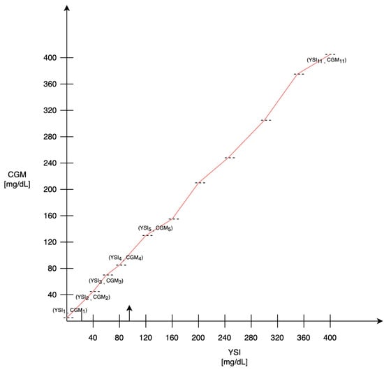 Figure 2. Sensor response, the dotted lines represent the extracted values, while the linear interpolation between these points is shown in red.To better describe this process, the algorithm is described with pseudocode (Algorithm 1). In the algorithm description, bins represents the number of intervals that can be defined in the YSI values, which in this specific case is equal to 11.
 - : the noise that affects the measure is defined as white noise with an amplitude included in of the measure.
- sensor response changes over time due to multiple factors, such as the biological body response that causes electrode oxidation and sensor degradation [19]. For these reasons, commercial sensors can measure glucose concentrations for a duration of 8–14 days depending on the type of device [20]. In this paper, the drift is modeled as a linear effect in which the slope of the line is obtained based on the range of values on the first day of observation, to simulate the effect reported in [21].
| Algorithm 1 Generate CGM Data Points with Adjusted Concentrations |
| Require:, YSI, mCGM, MCGM, P |
| Ensure: CGM, interpolator |
|
5.3. Model Evaluation
After producing the dataset as described in the previous section, the model is evaluated in terms of the distribution of obtained error and problem complexity. Two classic machine learning (ML) algorithms are presented, to understand the complexity of the problem: the Random Forest Regressor (RFR) and the Support Vector Regressor (SVR).
The RFR is based on multiple decision trees to predict a continuous outcome. It operates by constructing a multitude of decision trees at training time while outputting the average prediction of the individual trees to form a more accurate and robust prediction. It is widely used for various regression tasks due to its simplicity, ease of use, and ability to capture nonlinear relationships between features and the target variable.
The SVR is a type of Support Vector Machine (SVM) that is used for regression tasks. It works by finding the hyperplane that best fits the data in a high-dimensional space, trying to minimize the error within a certain margin. It is capable of capturing complex, nonlinear relationships by employing different kernel functions (linear, polynomial, radial basis function, etc.) to map input features into higher-dimensional spaces.
The RFR is evaluated considering different maximum values of parameters, referred to within the paper as max depth, in the range of 1–9, while SVR is evaluated using the linear kernel. For both the ML algorithms the Root Mean Square Error (RMSE), the Mean Absolute Error (MAE) and the are evaluated and compared.
All the analyses presented in this paper are performed considering the dataset that is reshaped into one-dimension array. Results were obtained on Google Colab using Python 3 on a A100 GPU (NVIDIA, Santa Clara, California, Stati Uniti) accelerated hardware.
Model on Specific Sensor
To evaluate the specificity of each sensor response, in this section, we analyze how the goodness of the sensor error response can be predicted given a single sensor output. This analysis was carried out using the RFR optimized in terms of MSE to get the number of estimators and parameters. After optimizing the model, it is applied to each record, which represents a sensor’s data collected over a 15-day period. Each derived dataset, indeed, is composed of a 500 × 2 matrix, where the first column represents the time and the second column the sensor error, while the ground truth is represented by the CGM value given by the simulator. Specifically, the initial 80% of the data trace from the specific sensor is employed to train the model. The remaining 20% of the data trace, which corresponds to the latter part of the recording period, is then used to test the model. This segment is particularly critical as it includes data where prediction errors can have more significant consequences, possibly due to the accumulation of small variances over time or abrupt changes in sensor behavior. This methodological approach of dividing the data are systematically applied across all 500 sensors involved in the study. Training and testing the model on these segmented portions of data from each sensor ensures that the model is both robust and capable of handling real-world variabilities in sensor outputs. Upon completion of the training and testing cycles, the MAE and MSE are calculated for each sensor’s predictions. The results are then aggregated to derive mean values and relative standard deviations for these metrics across all sensors. This statistical analysis provides a clear overview of the model’s overall accuracy and reliability in predicting sensor responses, highlighting its strengths and areas for potential improvement.
6. Result
The model is used to generate a dataset of 500 sensor responses for a duration of 15 days. The dataset has a final dimension of 500 × 7200. In Figure 3, there are a bunch of sensor responses in the range of 0–500 mg/dL overlapped over an ideal sensor response (dashed red line). Figure 4 shows a compact representation of all the 500 responses, where the blue line shows the average sensor response, and the area is the first and third quartile. It can be noticed that for low and high values of blood glucose concentration, the majority of measures cover a range wider than the region of interest (70–180 mg/dL).
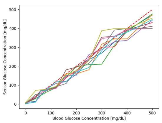
Figure 3.
10 sensor responses; the dashed line in red is the bisector that represents the ideal sensor response.
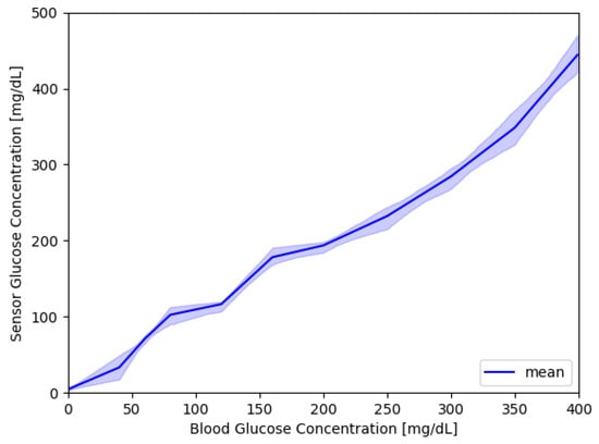
Figure 4.
500 sensor responses; the blue line shows the average sensor response, while the area covers the first and third quartile.
An example of a signal resulting from the model generated over the 15 days is shown in Figure 5, while a representation in terms of the mean and first and third quartile is reported in Figure 6. The absolute error grows over time reflecting the degradation of the sensor.
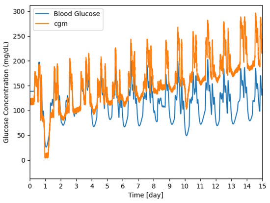
Figure 5.
Example of a signal generated by the model for 15 days; the CGM sensor response is shown in orange and the reference signal is shown in blue.
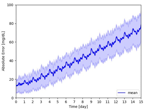
Figure 6.
Absolute glucose concentration error; the mean value over time is shown in blue, while the area represents the measures that are within the 25th and 75th percentile.
The absolute error evaluated as the average of every sensor response is expressed as Cumulative Distribution of Frequency (CDF), Figure 7. This graph shows that the error seems to be greater than zero. The distribution has a mean value of 40.79 mg/dL, with the 25th percentile at 21.02 mg/dL and the 75th percentile at 58.46 mg/dL.
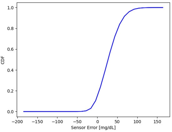
Figure 7.
Cumulative distribution of sensors error. Mean = mg/dL, the 25th percentile is at mg/dL, and the 75th percentile is at 58.46 mg/dL.
6.1. Model Evaluation
The dataset is reshaped in a one-dimensional array and it is splitted in train and test sets. The RFR model is trained using a max depth of 3 and 100 trees, while the SVR is trained with a linear kernel. Below the obtained results:
The results obtained with RFR are slightly better than SVR, although still not satisfactory for the pre-set task.
Regarding Table 2, the presented results may seem unusual, but this analysis was conducted to grasp the complexity of the problem. Deriving the relative value of blood glucose concentration from the sensor model using traditional machine learning algorithms is challenging. This difficulty highlights the complexity of the dataset and underscores the need for more advanced artificial intelligence algorithms.

Table 2.
Mean Square Error (), Mean Squared Error (), Mean Absolute Error (), and Coefficient of Determination () for RFR and SVR.
Model on the Specific Sensor
The last analysis made it possible to evaluate the performance of the trained models on the responses of individual sensors. The results obtained in terms of MSE is 223.93 ± 234.11 [(mg/dL)2] and MAE 11.01 ± 5.12 [mg/dL]. The latter result demonstrates the strong variability of traces within the dataset, whereby some specific models on some sensors perform very well, while others perform very poorly, as reported by the high standard deviation on the MSE metric.
7. Deployability on MCU
Considering that the CGM task requires an implementation of algorithms on a microcontroller (MCU) or a sensor itself, the definition of the mandatory requirements for the applicability of a model on such devices must be calculated. After choosing the max depth that results in less than 1% decrease in error, the portability of this model on the MCU is evaluated. From the graph shown in Figure 8, it is noticeable that by increasing max depth, there are no great improvements in terms of RMSE. This suggests that due to the complexity of the dataset, probably more complex algorithms of regression are needed.
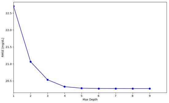
Figure 8.
RMSE evaluation for RF models with a variation of the model max depth parameter.
To assess the model’s portability on MCU, the STM32Cube.AI Developer Cloud tool [22] is utilized. This tool, freely available on the website, enables a machine learning developer to upload a pre-trained machine learning workload. Next, it allows to automatically profile its computational complexity and memory requirement. Then, it enables the automated ANSI C code conversion of the imported model. The C code is transparently integrated into a built-in application, which is then compiled and installed on the MCU chip. Finally, the installed firmware will be executed and detailed profiling (including the execution time) made available to the user. With this solution, it is possible to test the developed algorithm on the MCU chip. This tool facilitated the estimation of the selected model’s requirements, including the number of Multiply-Accumulate Operations (MACCs), as well as the needed flash memory, RAM space, and the inference time. The board U5855I is selected, due to its low power consumption (Arm Cortex-M33, 160 MHz, 768 KB of RAM for AI). The number of MACCs is 800, the flash needed is 24 KiB, including 15.43 KiB for network weights and about 8 KiB for libraries, and the total RAM is about 2 KiB. Benchmark on the selected board determined an inference time of 0.1920 ms. The complete result is shown in Table 3.

Table 3.
Details of algorithm implementation using the optimization of STM32Cube.AI Developer Cloud tool.
8. Discussion and Conclusions
Accurate monitoring of blood glucose is crucial for diabetes management and can significantly influence treatment decisions and patient well-being. A dataset that accurately mimics the behavior of an array of sensor types becomes an essential tool for progress. Such a dataset aids in developing robust machine-learning algorithms that can handle intrinsic variability and potential sensor degradation. Traditional machine learning methods, such as RFR and SVR, show promise but also exhibit limitations, particularly regarding systematic and random errors even when these are trained on data from individual sensors reveal that the outcome is heavily dependent on the quality of the initial signal. This is probably due to the complexity of the task. One of the goals of this paper is to characterize the complexity of the generated dataset. While the presented analysis aligns with the model analyses presented in [9], which are based on real-world data, it demonstrates greater complexity compared to [11]. Unlike the existing literature, which primarily relies on real data, the presented approach is novel in that it utilizes simulated data to perform stress tests.
The primary contribution of this paper is the development of a method to generate datasets enabling the test of calibration and self-calibration strategies under a vast variety of error conditions. This simulated data approach allows for a rigorous evaluation of DSP and ML processing algorithms even under extreme sensor working conditions.
The presented dataset holds substantial promise, as it simulates various interfering factors that affect glucose measurement. The quality of the produced data, indeed, is tunable based on adjustable disturbance levels connected to real-world conditions over short and long time frames. This enriches the machine learning models’ training process, enabling a comprehensive understanding of sensor errors and allowing for the development of more precise algorithms. This not only furthers our understanding of sensor inaccuracies, but also paves the way for advanced glucose monitoring systems. Future models that effectively compensate for signal variability and improve glucose detection could greatly enhance the management of diabetes, thus potentially improving the quality of life for individuals with this condition.
Author Contributions
Conceptualization, D.P. and L.V.; methodology, A.S., D.P. and L.V.; software, A.S. and C.C.; validation, A.S. and C.C.; formal analysis, L.V. and D.P.; writing—original draft preparation, A.S. and C.C.; writing—review and editing, L.V. and D.P.; supervision, L.V. and D.P. All authors have read and agreed to the published version of the manuscript.
Funding
This research received no external funding and Anna Sabatini is funded by PON “Ricerca e Innovazione” 2014–2020.
Institutional Review Board Statement
Not applicable.
Informed Consent Statement
Not applicable.
Data Availability Statement
Data are available after request to the author.
Conflicts of Interest
Author Danilo Pau was employed by the company STMicroelectronics. The remaining authors declare that the research was conducted in the absence of any commercial or financial relationships that could be construed as a potential conflict of interest.
References
- World Health Organization. Available online: https://www.who.int/health-topics/diabetes#tab=tab_1 (accessed on 3 April 2023).
- Basu, S.; Yudkin, J.S. Estimation of global insulin use for type 2 diabetes, 2018-30: A microsimulation analysis. Lancet Diabetes Endocrinol. 2018, 7, 25–33. [Google Scholar] [CrossRef] [PubMed]
- International Diabetes Federation. Diabetes Facts & Figures. Sito Web. Available online: https://idf.org/about-diabetes/diabetes-facts-figures/ (accessed on 26 March 2024).
- Dovc, K.; Battelino, T. Time in range centered diabetes care. Clin. Pediatr. Endocrinol. 2021, 30, 1–10. [Google Scholar] [CrossRef] [PubMed]
- Heinemann, L. Continuous Glucose Monitoring (CGM) or Blood Glucose Monitoring (BGM): Interactions and Implications. J. Diabetes Sci. Technol. 2018, 12, 873–879. [Google Scholar] [CrossRef]
- Martens, T.; Beck, R.W.; Bailey, R.; Ruedy, K.J.; Calhoun, P.; Peters, A.L.; Pop-Busui, R.; Philis-Tsimikas, A.; Bao, S.; Umpierrez, G.; et al. Effect of Continuous Glucose Monitoring on Glycemic Control in Patients With Type 2 Diabetes Treated With Basal Insulin: A Randomized Clinical Trial. JAMA 2021, 325, 2262–2272. [Google Scholar] [CrossRef]
- Luijf, Y.M.; Mader, J.K.; Doll, W.; Pieber, T.; Farret, A.; Place, J.; Renard, E.; Bruttomesso, D.; Filippi, A.; Avogaro, A.; et al. Accuracy and reliability of continuous glucose monitoring systems: A head-to-head comparison. Diabetes Technol. Ther. 2013, 15, 722–727. [Google Scholar] [CrossRef]
- Krouwer, J.S.; Cembrowski, G.S. A review of standards and statistics used to describe blood glucose monitor performance. J. Diabetes Sci. Technol. 2010, 4, 75–83. [Google Scholar] [CrossRef]
- Facchinetti, A.; Del Favero, S.; Sparacino, G.; Castle, J.R.; Ward, W.K.; Cobelli, C. Modeling the glucose sensor error. IEEE Trans. Biomed. Eng. 2013, 61, 620–629. [Google Scholar] [CrossRef] [PubMed]
- Facchinetti, A.; Del Favero, S.; Sparacino, G.; Cobelli, C. Model of glucose sensor error components: Identification and assessment for new Dexcom G4 generation devices. Med. Biol. Eng. Comput. 2015, 53, 1259–1269. [Google Scholar] [CrossRef] [PubMed]
- Vettoretti, M.; Del Favero, S.; Sparacino, G.; Facchinetti, A. Modeling the error of factory-calibrated continuous glucose monitoring sensors: Application to Dexcom G6 sensor data. In Proceedings of the 2019 41st Annual International Conference of the IEEE Engineering in Medicine and Biology Society (EMBC), Berlin, Germany, 23–27 July 2019; pp. 750–753. [Google Scholar]
- Liu, C.; Vehí, J.; Avari, P.; Reddy, M.; Oliver, N.; Georgiou, P.; Herrero, P. Long-term glucose forecasting using a physiological model and deconvolution of the continuous glucose monitoring signal. Sensors 2019, 19, 4338. [Google Scholar] [CrossRef] [PubMed]
- Drecogna, M.; Vettoretti, M.; Del Favero, S.; Facchinetti, A.; Sparacino, G. Data gap modeling in continuous glucose monitoring sensor data. In Proceedings of the 2021 43rd Annual International Conference of the IEEE Engineering in Medicine & Biology Society (EMBC), Mexico City, Mexico, 1–5 November 2021; pp. 4379–4382. [Google Scholar]
- Talukder, S.; Kundu, S.; Kumar, R. Dynamic Calibration of Nonlinear Sensors with Time-Drifts and Delays by Bayesian Inference. arXiv 2022, arXiv:2208.13819. [Google Scholar]
- Xie, J. Simglucose v0.2.1. 2018. Available online: https://github.com/jxx123/simglucose (accessed on 21 March 2024).
- Schiavon, M.; Dalla Man, C.; Dube, S.; Slama, M.; Kudva, Y.C.; Peyser, T.; Basu, A.; Basu, R.; Cobelli, C. Modeling plasma-to-interstitium glucose kinetics from multitracer plasma and microdialysis data. Diabetes Technol. Ther. 2015, 17, 825–831. [Google Scholar] [CrossRef] [PubMed]
- Acciaroli, G.; Vettoretti, M.; Facchinetti, A.; Sparacino, G. Calibration of CGM systems. In Glucose Monitoring Devices; Elsevier: Amsterdam, The Netherlands, 2020; pp. 173–201. [Google Scholar]
- Dexcom, I. User Guide G7. 2023. Available online: https://dexcompdf.s3.us-west-2.amazonaws.com/en-us/G7-CGM-Users-Guide.pdf (accessed on 10 March 2024).
- Alva, S.; Bailey, T.; Brazg, R.; Budiman, E.S.; Castorino, K.; Christiansen, M.P.; Forlenza, G.; Kipnes, M.; Liljenquist, D.R.; Liu, H. Accuracy of a 14-day factory-calibrated continuous glucose monitoring system with advanced algorithm in pediatric and adult population with diabetes. J. Diabetes Sci. Technol. 2022, 16, 70–77. [Google Scholar] [CrossRef] [PubMed]
- Das, S.K.; Nayak, K.K.; Krishnaswamy, P.; Kumar, V.; Bhat, N. Electrochemistry and other emerging technologies for continuous glucose monitoring devices. ECS Sensors Plus 2022, 1, 031601. [Google Scholar]
- Acciaroli, G.; Vettoretti, M.; Facchinetti, A.; Sparacino, G. Calibration of minimally invasive continuous glucose monitoring sensors: State-of-the-art and current perspectives. Biosensors 2018, 8, 24. [Google Scholar] [CrossRef] [PubMed]
- STM32Cube.AI Developer Cloud. Available online: https://stm32ai-cs.st.com/home (accessed on 3 April 2024).
Disclaimer/Publisher’s Note: The statements, opinions and data contained in all publications are solely those of the individual author(s) and contributor(s) and not of MDPI and/or the editor(s). MDPI and/or the editor(s) disclaim responsibility for any injury to people or property resulting from any ideas, methods, instructions or products referred to in the content. |
© 2024 by the authors. Licensee MDPI, Basel, Switzerland. This article is an open access article distributed under the terms and conditions of the Creative Commons Attribution (CC BY) license (https://creativecommons.org/licenses/by/4.0/).